
Note: in more recent versions of Excel, the FILTER function is a better way to solve this problem. The INDEX and MATCH formula explained here is meant for legacy versions of Excel that do not provide the FILTER function.
By default, lookup formulas in Excel like VLOOKUP and INDEX + MATCH will find the first match, but not other matches that may exist in a set of data. However, with some effort, you can make INDEX and MATCH return all matches. One way to approach this problem is to use a helper column to return a numeric value that indicates a match. This makes it much easier to identify and extract multiple matches.
Helper column
A helper column is a way to simplify a complex formula in Excel by breaking the problem down into smaller steps. In the worksheet shown, a helper column is used to identify matching data based on conditions entered in the range I3:J3. The formula in the helper column in cell E3 looks like this:
=SUM(E2,AND(C3=$I$3,D3=$J$3))
The helper column tests each row in the data to see if the Department in column C matches the value in I3 and the Building in column D matches the value in J3. Both logical tests must return TRUE in order for AND to return TRUE.
For each row, the result from the AND function is added to the «value above» in the helper column to generate a count. The practical effect of this formula is an incrementing counter that only changes when a (new) match is found. Then the value remains the same until the next match is found. This works because the TRUE/FALSE results return by AND are coerced to 1/0 values as part of the sum operation. FALSE results add nothing and TRUE results add 1.
Back in the extraction area, the lookup formula for Name in column H looks like this:
=IF($G6<=ct,INDEX(data,MATCH($G6,helper,0),1),"")
Working from the inside out, the INDEX + MATCH part of the formula looks up the name for the first match found, using the row number in column G as the match value:
INDEX(data,MATCH($G6,helper,0),1)
INDEX receives all 3 columns of data as the array (named range «data»), and MATCH is configured to match the row number inside the helper column (the named range «helper») in exact match mode (3rd argument set to zero).
This is where the cleverness of the formula becomes apparent. The helper column obviously contains duplicates, but it doesn’t matter, because MATCH will match only the first value. By design, each «first value» corresponds to the correct row in the data table.
The formulas in columns I and J are the same as H, except for the column number, which is increased in each case by one.
The IF statement that wraps the INDEX/MATCH formula performs a simple function — it checks each row number in the extraction area to see if the row number is less than or equal to the value in G3 (named range «ct»), which is the total count of all matching records. If so, the INDEX/MATCH logic is run. If not, IF outputs an empty string («»).
The formula in G3 (named range «ct») is simple:
=MAX(helper)
Since the maximum value in the helper column is the same as the total match count, the MAX function is all we need.
Note: the extraction area needs to be manually configured to handle as much data as needed (i.e. 5 rows, 10 rows, 20 rows, etc.). In this example, it is limited to 5 rows only to keep the worksheet compact.
I learned this technique in Mike Girvin’s book Control + Shift + Enter.
The FILTER function
If you have a current version of Excel, the FILTER function is a better way to extract all matching records.
Tip: Try using the new XLOOKUP and XMATCH functions, improved versions of the functions described in this article. These new functions work in any direction and return exact matches by default, making them easier and more convenient to use than their predecessors.
Suppose that you have a list of office location numbers, and you need to know which employees are in each office. The spreadsheet is huge, so you might think it is challenging task. It’s actually quite easy to do with a lookup function.
The VLOOKUP and HLOOKUP functions, together with INDEX and MATCH, are some of the most useful functions in Excel.
Note: The Lookup Wizard feature is no longer available in Excel.
Here’s an example of how to use VLOOKUP.
=VLOOKUP(B2,C2:E7,3,TRUE)
In this example, B2 is the first argument—an element of data that the function needs to work. For VLOOKUP, this first argument is the value that you want to find. This argument can be a cell reference, or a fixed value such as «smith» or 21,000. The second argument is the range of cells, C2-:E7, in which to search for the value you want to find. The third argument is the column in that range of cells that contains the value that you seek.
The fourth argument is optional. Enter either TRUE or FALSE. If you enter TRUE, or leave the argument blank, the function returns an approximate match of the value you specify in the first argument. If you enter FALSE, the function will match the value provide by the first argument. In other words, leaving the fourth argument blank—or entering TRUE—gives you more flexibility.
This example shows you how the function works. When you enter a value in cell B2 (the first argument), VLOOKUP searches the cells in the range C2:E7 (2nd argument) and returns the closest approximate match from the third column in the range, column E (3rd argument).
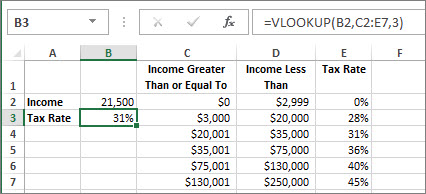
The fourth argument is empty, so the function returns an approximate match. If it didn’t, you’d have to enter one of the values in columns C or D to get a result at all.
When you’re comfortable with VLOOKUP, the HLOOKUP function is equally easy to use. You enter the same arguments, but it searches in rows instead of columns.
Using INDEX and MATCH instead of VLOOKUP
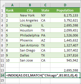
There are certain limitations with using VLOOKUP—the VLOOKUP function can only look up a value from left to right. This means that the column containing the value you look up should always be located to the left of the column containing the return value. Now if your spreadsheet isn’t built this way, then do not use VLOOKUP. Use the combination of INDEX and MATCH functions instead.
This example shows a small list where the value we want to search on, Chicago, isn’t in the leftmost column. So, we can’t use VLOOKUP. Instead, we’ll use the MATCH function to find Chicago in the range B1:B11. It’s found in row 4. Then, INDEX uses that value as the lookup argument, and finds the population for Chicago in the 4th column (column D). The formula used is shown in cell A14.
For more examples of using INDEX and MATCH instead of VLOOKUP, see the article https://www.mrexcel.com/excel-tips/excel-vlookup-index-match/ by Bill Jelen, Microsoft MVP.
Give it a try
If you want to experiment with lookup functions before you try them out with your own data, here’s some sample data.
VLOOKUP Example at work
Copy the following data into a blank spreadsheet.
Tip: Before you paste the data into Excel, set the column widths for columns A through C to 250 pixels, and click Wrap Text (Home tab, Alignment group).
|
Density |
Viscosity |
Temperature |
|
0.457 |
3.55 |
500 |
|
0.525 |
3.25 |
400 |
|
0.606 |
2.93 |
300 |
|
0.675 |
2.75 |
250 |
|
0.746 |
2.57 |
200 |
|
0.835 |
2.38 |
150 |
|
0.946 |
2.17 |
100 |
|
1.09 |
1.95 |
50 |
|
1.29 |
1.71 |
0 |
|
Formula |
Description |
Result |
|
=VLOOKUP(1,A2:C10,2) |
Using an approximate match, searches for the value 1 in column A, finds the largest value less than or equal to 1 in column A which is 0.946, and then returns the value from column B in the same row. |
2.17 |
|
=VLOOKUP(1,A2:C10,3,TRUE) |
Using an approximate match, searches for the value 1 in column A, finds the largest value less than or equal to 1 in column A, which is 0.946, and then returns the value from column C in the same row. |
100 |
|
=VLOOKUP(0.7,A2:C10,3,FALSE) |
Using an exact match, searches for the value 0.7 in column A. Because there is no exact match in column A, an error is returned. |
#N/A |
|
=VLOOKUP(0.1,A2:C10,2,TRUE) |
Using an approximate match, searches for the value 0.1 in column A. Because 0.1 is less than the smallest value in column A, an error is returned. |
#N/A |
|
=VLOOKUP(2,A2:C10,2,TRUE) |
Using an approximate match, searches for the value 2 in column A, finds the largest value less than or equal to 2 in column A, which is 1.29, and then returns the value from column B in the same row. |
1.71 |
HLOOKUP Example
Copy all the cells in this table and paste it into cell A1 on a blank worksheet in Excel.
Tip: Before you paste the data into Excel, set the column widths for columns A through C to 250 pixels, and click Wrap Text (Home tab, Alignment group).
|
Axles |
Bearings |
Bolts |
|
4 |
4 |
9 |
|
5 |
7 |
10 |
|
6 |
8 |
11 |
|
Formula |
Description |
Result |
|
=HLOOKUP(«Axles», A1:C4, 2, TRUE) |
Looks up «Axles» in row 1, and returns the value from row 2 that’s in the same column (column A). |
4 |
|
=HLOOKUP(«Bearings», A1:C4, 3, FALSE) |
Looks up «Bearings» in row 1, and returns the value from row 3 that’s in the same column (column B). |
7 |
|
=HLOOKUP(«B», A1:C4, 3, TRUE) |
Looks up «B» in row 1, and returns the value from row 3 that’s in the same column. Because an exact match for «B» is not found, the largest value in row 1 that is less than «B» is used: «Axles,» in column A. |
5 |
|
=HLOOKUP(«Bolts», A1:C4, 4) |
Looks up «Bolts» in row 1, and returns the value from row 4 that’s in the same column (column C). |
11 |
|
=HLOOKUP(3, {1,2,3;»a»,»b»,»c»;»d»,»e»,»f»}, 2, TRUE) |
Looks up the number 3 in the three-row array constant, and returns the value from row 2 in the same (in this case, third) column. There are three rows of values in the array constant, each row separated by a semicolon (;). Because «c» is found in row 2 and in the same column as 3, «c» is returned. |
c |
INDEX and MATCH Examples
This last example employs the INDEX and MATCH functions together to return the earliest invoice number and its corresponding date for each of five cities. Because the date is returned as a number, we use the TEXT function to format it as a date. The INDEX function actually uses the result of the MATCH function as its argument. The combination of the INDEX and MATCH functions are used twice in each formula – first, to return the invoice number, and then to return the date.
Copy all the cells in this table and paste it into cell A1 on a blank worksheet in Excel.
Tip: Before you paste the data into Excel, set the column widths for columns A through D to 250 pixels, and click Wrap Text (Home tab, Alignment group).
|
Invoice |
City |
Invoice Date |
Earliest invoice by city, with date |
|
3115 |
Atlanta |
4/7/12 |
=»Atlanta = «&INDEX($A$2:$C$33,MATCH(«Atlanta»,$B$2:$B$33,0),1)& «, Invoice date: » & TEXT(INDEX($A$2:$C$33,MATCH(«Atlanta»,$B$2:$B$33,0),3),»m/d/yy») |
|
3137 |
Atlanta |
4/9/12 |
=»Austin = «&INDEX($A$2:$C$33,MATCH(«Austin»,$B$2:$B$33,0),1)& «, Invoice date: » & TEXT(INDEX($A$2:$C$33,MATCH(«Austin»,$B$2:$B$33,0),3),»m/d/yy») |
|
3154 |
Atlanta |
4/11/12 |
=»Dallas = «&INDEX($A$2:$C$33,MATCH(«Dallas»,$B$2:$B$33,0),1)& «, Invoice date: » & TEXT(INDEX($A$2:$C$33,MATCH(«Dallas»,$B$2:$B$33,0),3),»m/d/yy») |
|
3191 |
Atlanta |
4/21/12 |
=»New Orleans = «&INDEX($A$2:$C$33,MATCH(«New Orleans»,$B$2:$B$33,0),1)& «, Invoice date: » & TEXT(INDEX($A$2:$C$33,MATCH(«New Orleans»,$B$2:$B$33,0),3),»m/d/yy») |
|
3293 |
Atlanta |
4/25/12 |
=»Tampa = «&INDEX($A$2:$C$33,MATCH(«Tampa»,$B$2:$B$33,0),1)& «, Invoice date: » & TEXT(INDEX($A$2:$C$33,MATCH(«Tampa»,$B$2:$B$33,0),3),»m/d/yy») |
|
3331 |
Atlanta |
4/27/12 |
|
|
3350 |
Atlanta |
4/28/12 |
|
|
3390 |
Atlanta |
5/1/12 |
|
|
3441 |
Atlanta |
5/2/12 |
|
|
3517 |
Atlanta |
5/8/12 |
|
|
3124 |
Austin |
4/9/12 |
|
|
3155 |
Austin |
4/11/12 |
|
|
3177 |
Austin |
4/19/12 |
|
|
3357 |
Austin |
4/28/12 |
|
|
3492 |
Austin |
5/6/12 |
|
|
3316 |
Dallas |
4/25/12 |
|
|
3346 |
Dallas |
4/28/12 |
|
|
3372 |
Dallas |
5/1/12 |
|
|
3414 |
Dallas |
5/1/12 |
|
|
3451 |
Dallas |
5/2/12 |
|
|
3467 |
Dallas |
5/2/12 |
|
|
3474 |
Dallas |
5/4/12 |
|
|
3490 |
Dallas |
5/5/12 |
|
|
3503 |
Dallas |
5/8/12 |
|
|
3151 |
New Orleans |
4/9/12 |
|
|
3438 |
New Orleans |
5/2/12 |
|
|
3471 |
New Orleans |
5/4/12 |
|
|
3160 |
Tampa |
4/18/12 |
|
|
3328 |
Tampa |
4/26/12 |
|
|
3368 |
Tampa |
4/29/12 |
|
|
3420 |
Tampa |
5/1/12 |
|
|
3501 |
Tampa |
5/6/12 |
In this article, we will learn how to Lookup & SUM values with INDEX and MATCH function in Excel.
For the formula to understand first we need to revise a little about the three functions
- SUM
- INDEX
- MATCH
SUM function adds all the numbers in a range of cells and returns the sum of these values.
INDEX function returns the value at a given index in an array.
MATCH function returns the index of the first appearance of the value in an array ( single dimension array ).
Now we will make a formula using the above functions. Match function will return the index of the lookup value in the header field. The index number will now be fed to the INDEX function to get the values under the lookup value.
Then the SUM function will return the sum from the found values.
Use the Formula:
= SUM ( INDEX ( data , 0, MATCH ( lookup_value, headers, 0)))
The above statements can be complicated to understand. So let’s understand this by using the formula in an example
Here we have a list of marks of students and we need to find the total marks for a specific person (Gary) as shown in the snapshot below.
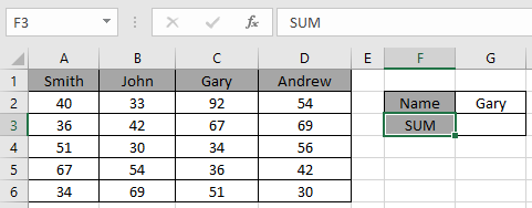
Use the formula in the C2 cell:
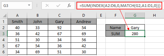
= SUM ( INDEX ( A2:D6 , 0 , MATCH ( G2 , A1:D1 , 0 )))
Explanation:
- The MATCH function matches the first value with the header array and returns its position 3 as a number.
- The INDEX function takes the number as the column index for the data and returns the array { 92 ; 67 ; 34 ; 36 ; 51 } to the argument of the SUM function
- The SUM function takes the array and returns the SUM in the cell.
Here values to the function is given as cell reference.
As you can see in the above snapshot, we got the SUM of the marks of student Gary. And it proves the formula works fine and for doubts see the below notes for understanding.
Notes:
- The function returns the #NA error if the lookup array argument to the MATCH function is 2 — D array which is the header field of the data..
- The function matches exact value as the match type argument to the MATCH function is 0.
- The lookup value can be given as cell reference or directly using quote symbol («).
- The SUM function ignores the text values in the array received from the INDEX function.
Hope you understood how to use the LOOKUP function in Excel. Explore more articles on Excel lookup value here. Please feel free to state your queries below in the comment box. We will certainly help you.
Related Articles
Use INDEX and MATCH to Lookup Value
SUM range with INDEX in Excel
How to use the SUM function in Excel
How to use the INDEX function in Excel
How to use the MATCH function in Excel
How to use LOOKUP function in Excel
How to use the VLOOKUP function in Excel
How to use the HLOOKUP function in Excel
Popular Articles
Edit a dropdown list
If with conditional formatting
If with wildcards
Vlookup by date
Excel has a lot of functions – about 450+ of them.
And many of these are simply awesome. The amount of work you can get done with a few formulas still surprises me (even after having used Excel for 10+ years).
And among all these amazing functions, the INDEX MATCH functions combo stands out.
I am a huge fan of INDEX MATCH combo and I have made it pretty clear many times.
I even wrote an article about Index Match Vs VLOOKUP which sparked a little bit of debate (you can check the comments section for some firework).
And today, I am writing this article solely focussed on Index Match to show you some simple and advanced scenarios where you can use this powerful formula combo and get the work done.
Note: There are other lookup formulas in Excel – such as VLOOKUP and HLOOKUP and these are great. Many people find VLOOKUP to be easier to use (and that’s true as well). I believe INDEX MATCH is a better option in many cases. But since people find it difficult, it gets used less. So I am trying to simplify it using this tutorial.
Now before I show you how the combination of INDEX MATCH is changing the world of analysts and data scientists, let me first introduce you to the individual parts – INDEX and MATCH functions.
INDEX Function: Finds the Value-Based on Coordinates
The easiest way to understand how Index function works is by thinking of it as a GPS satellite.
As soon as you tell the satellite the latitude and longitude coordinates, it will know exactly where to go and find that location.
So despite having a mind-boggling number of lat-long combinations, the satellite would know exactly where to look.
I quickly did a search for my work location and this is what I got.
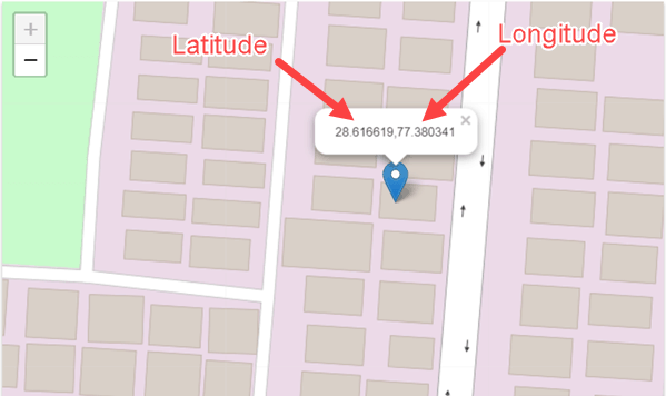
Anyway, enough of geography.
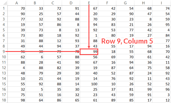
Just like a satellite needs latitude and longitude coordinates, the INDEX function in Excel would need the row and column number to know what cell you’re referring to.
And that’s Excel INDEX function in a nut-shell.
So let me define it in simple words for you.
The INDEX function will use the row number and column number to find a cell in the given range and return the value in it.
All by itself, INDEX is a very simple function, with no utility. After all, in most cases, you are not likely to know the row and column numbers.
But…
The fact that you can use it with other functions (hint: MATCH) that can find the row number and the column number makes INDEX an extremely powerful Excel function.
Below is the syntax of the INDEX function:
=INDEX (array, row_num, [col_num])
=INDEX (array, row_num, [col_num], [area_num])
- array – a range of cells or an array constant.
- row_num – the row number from which the value is to be fetched.
- [col_num] – the column number from which the value is to be fetched. Although this is an optional argument, but if row_num is not provided, it needs to be given.
- [area_num] – (Optional) If array argument is made up of multiple ranges, this number would be used to select the reference from all the ranges.
INDEX function has 2 syntaxes (just FYI).
The first one is used in most cases. The second one is used in advanced cases only (such as doing a three-way lookup) which we will cover in one of the examples later in this tutorial.
But if you’re new to this function, just remember the first syntax.
Below is a video that explains how to use the INDEX function
MATCH Function: Finds the Position baed on a Lookup Value
Going back to my previous example of longitude and latitude, MATCH is the function that can find these positions (in the Excel spreadsheet world).
In simple language, the Excel MATCH function can find the position of a cell in a range.
And on what basis would it find a cell’s position?
Based on the lookup value.
For example, if you have a list as shown below and you want to find the position of the name ‘Mark’ in it, then you can use the MATCH function.
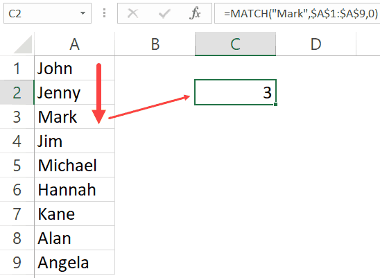
The function returns 3, as that’s the position of the cell with the name Mark in it.
MATCH function starts looking from top to bottom for the lookup value (which is ‘Mark’) in the specified range (which is A1:A9 in this example). As soon as it finds the name, it returns the position in that specific range.
Below is the syntax of the MATCH function in Excel.
=MATCH(lookup_value, lookup_array, [match_type])
- lookup_value – The value for which you are looking for a match in the lookup_array.
- lookup_array – The range of cells in which you are searching for the lookup_value.
- [match_type] – (Optional) This specifies how excel should look for a matching value. It can take three values -1, 0 , or 1.
Understanding Match Type Argument in MATCH Function
There is one additional thing you need to know about the MATCH function, and it’s about how it goes through the data and finds the cell position.
The third argument of the MATCH function can be 0, 1 or -1.
Below is an explanation of how these arguments work:
- 0 – this will look for an exact match of the value. If an exact match is found, the MATCH function will return the cell position. Else, it will return an error.
- 1 – this finds the largest value that is less than or equal to the lookup value. For this to work, your data range needs to be sorted in ascending order.
- -1 – this finds the smallest value that is greater than or equal to the lookup value. For this to work, your data range needs to be sorted in descending order.
Below is a video that explains how to use the MATCH function (along with the match type argument)
To summarize and put it in simple words:
- INDEX needs the cell position (row and column number) and gives the cell value.
- MATCH finds the position by using a lookup value.
Let’s Combine Them to Create a Powerhouse (INDEX + MATCH)
Now that you have a basic understanding of how INDEX and MATCH functions work individually, let’s combine these two and learn about all the wonderful things it can do.
To understand this better, I have a few examples that use the INDEX MATCH combination.
I will start with a simple example and then show you some advanced use cases as well.
Click here to download the example file
Example 1: A simple Lookup Using INDEX MATCH Combo
Let’s do a simple lookup with INDEX/MATCH.
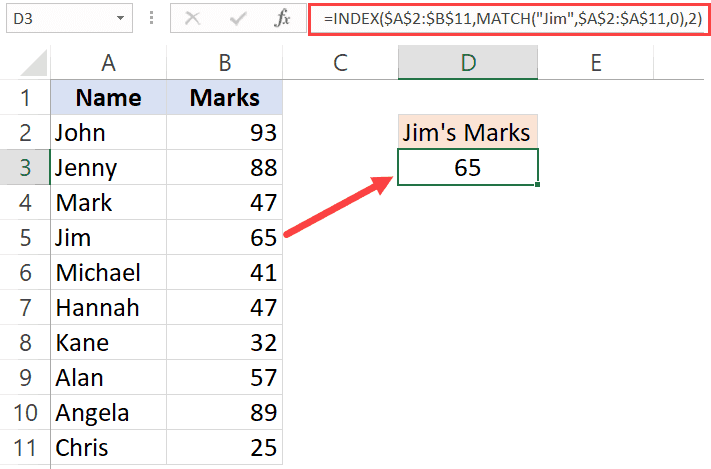
Below is a table where I have the marks for ten students.
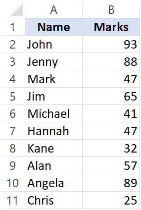
From this table, I want to find the marks for Jim.
Below is the formula that can easily do this:
=INDEX($A$2:$B$11,MATCH("Jim",$A$2:$A$11,0),2)
Now, if you’re thinking this can easily be done using a VLOOKUP function, you’re right! This is not the best use of INDEX MATCH awesomeness. Despite the fact that I am a fan of INDEX MATCH, it is a little more difficult than VLOOKUP. If fetching data from a column on the right is all you want to do, I recommend you use VLOOKUP.
The reason I have shown this example, which can also easily be done with VLOOKUP is to show you how INDEX MATCH works in a simple setting.
Now let me show a benefit of INDEX MATCH.
Suppose you have the same data, but instead of having it in columns, you have it in rows (as shown below).

You know what, you can still use INDEX MATCH combo to get Jim’s marks.
Below is the formula that will give you the result:
=INDEX($B$1:$K$2,2,MATCH(“Jim”,$B$1:$K$1,0))
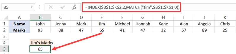
Note that you need to change the range and switch the row/column parts to make this formula work for horizontal data as well.
This can’t be done with VLOOKUP, but you can still do this easily with HLOOKUP.
INDEX MATCH combination can easily handle horizontal as well as vertical data.
Click here to download the example file
Example 2: Lookup to the Left
It’s more common than you think.
A lot of times, you may be required to fetch the data from a column which is to the left of the column that has the lookup value.
Something as shown below:
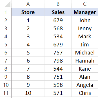
To find out Michael’s sales, you will have to do a lookup on the left.
If you’re thinking VLOOKUP, let me stop your right there.
VLOOKUP is not made to look for and fetch the values on the left.
Can you still do it using VLOOKUP?
Yes, you can!
But that can turn into a long and ugly formula.
So if you want to do a lookup and fetch data from the columns on the left, you are better off using INDEX MATCH combo.
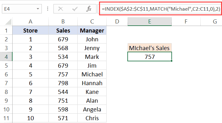
Below is the formula that will get Michael’s sales number:
=INDEX($A$2:$C$11,MATCH("Michael",C2:C11,0),2)
Another point here for INDEX MATCH. VLOOKUP can fetch the data only from the columns that are to the right of the column that has the lookup value.
Example 3: Two Way Lookup
So far, we have seen the examples where we wanted to fetch the data from the column adjacent to the column that has the lookup value.
But in real life, the data often spans through multiple columns.
INDEX MATCH can easily handle a two-way lookup.
Below is a dataset of the student’s marks in three different subjects.
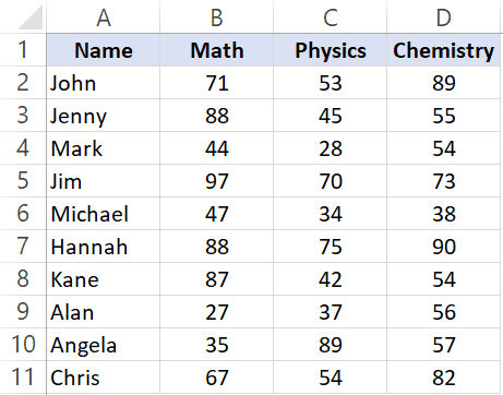
If you want to quickly fetch the marks of a student in all three subjects, you can do that with INDEX MATCH.
The below formula will give you the marks for Jim for all the three subjects (copy and paste in one cell and drag to fill other cells or copy and paste on other cells).
=INDEX($B$2:$D$11,MATCH($F$3,$A$2:$A$11,0),MATCH(G$2,$B$1:$D$1,0))

Let me quickly also explain this formula.
INDEX formula uses B2:D11 as the range.
The first MATCH uses the name (Jim in cell F3) and fetches the position of it in the names column (A2:A11). This becomes the row number from which the data needs to be fetched.
The second MATCH formula uses the subject name (in cell G2) to get the position of that specific subject name in B1:D1. For example, Math is 1, Physics is 2 and Chemistry is 3.
Since these MATCH positions are fed into the INDEX function, it returns the score based on the student name and subject name.
This formula is dynamic, which means that if you change the student name or the subject names, it would still work and fetch the correct data.
One great thing about using INDEX/MATCH is that even if you interchange the names of the subjects, it will continue to give you the correct result.
Example 4: Lookup Value From Multiple Column/Criteria
Suppose you have a dataset as shown below and you want to fetch the marks for ‘Mark Long’.

Since the data is in two columns, I can’t a lookup for Mark and get the data.
If I do it that way, I am going to get the marks data for Mark Frost and not Mark Long (because the MATCH function will give me the result for the MARK it meets).
One way of doing this is to create a helper column and combine the names. Once you have the helper column, you can use VLOOKUP and get the marks data.
If you’re interested in learning how to do this, read this tutorial on using VLOOKUP with multiple criteria.
But with INDEX/MATCH combo, you don’t need a helper column. You can create a formula that handles multiple criteria in the formula itself.
The below formula will give the result.
=INDEX($C$2:$C$11,MATCH($E$3&"|"&$F$3,$A$2:A11&"|"&$B$2:$B$11,0))

Let me quickly explain what this formula does.
The MATCH part of the formula combines the lookup value (Mark and Long) as well as the entire lookup array. When $A$2:A11&”|”&$B$2:$B$11 is used as the lookup array, it actually checks the lookup value against the combined string of first and last name (separated by the pipe symbol).
This ensures that you get the right result without using any helper columns.
You can do this kind of lookup (where there are multiple columns/criteria) with VLOOKUP as well, but you need to use a helper column. INDEX MATCH combo makes it slightly easy to do this without any helper columns.
Example 5: Get Values from Entire Row/Column
In the examples above, we have used the INDEX function to get value from a specific cell. You provide the row and column number, and it returns the value in that specific cell.
But you can do more.
You can also use the INDEX function to get the values from an entire row or column.
And how can this be useful you ask!
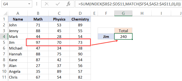
Suppose you want to know the total score of Jim in all the three subjects.
You can use the INDEX function to first get all the marks of Jim and then use the SUM function to get a total.
Let’s see how to do this.
Below I have the scores of all the students in three subjects.
The below formula will give me the total score of Jim in all the three subjects.
=SUM(INDEX($B$2:$D$11,MATCH($F$4,$A$2:$A$11,0),0))
Let me explain how this formula works.
The trick here is to use 0 as the column number.
When you use 0 as the column number in the INDEX function, it will return all the row values. Similarly, if you use 0 as the row number, it will return all the values in the column.
So the below part of the formula returns an array of values – {97, 70, 73}
INDEX($B$2:$D$11,MATCH($F$4,$A$2:$A$11,0),0)
If you just enter this above formula in a cell in Excel and hit enter, you will see a #VALUE! error. This is because it’s not returning a single value, but an array of value.
But don’t worry, the array of values are still there. You can check this by selecting the formula and press the F9 key. It will show you the result of the formula which in this case is an array of three value – {97, 70, 73}
Now, if you wrap this INDEX formula in the SUM function, it will give you the sum of all the marks scored by Jim.
You can also use the same to get the highest, lowest and average marks of Jim.
Just like we have done this for a student, you can also do this for a subject. For example, if you want the average score in a subject, you can keep the row number as 0 in the INDEX formula and it will give you all the column values of that subject.
Click here to download the example file
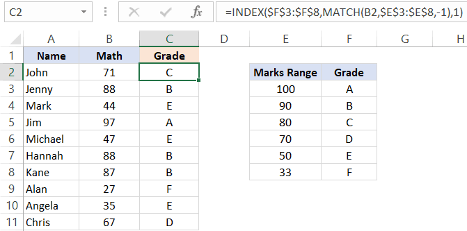
Example 6: Find the Student’s Grade (Approximate Match Technique)
So far, we have used the MATCH formula to get the exact match of the lookup value.
But you can also use it to do an approximate match.
Now, what the hell is Approximate Match?
Let me explain.
When you’re looking for stuff such as names or ids, you’re looking for an exact match. But sometimes, you need to know the range in which your lookup values lie. This is usually the case with numbers.
For example, as a class teacher, you may want to know what’s the grade of each student in a subject, and the grade is decided based on the score.
Below is an example, where I want the grade for all the students and the grading is decided based on the table on the right.
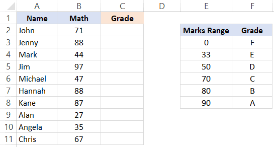
So if a student gets less than 33, the grade is F and if he/she gets less than 50 but more than 33, it’s E, and so on.
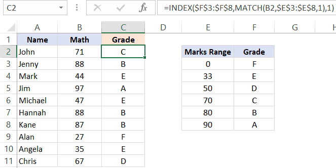
Below is the formula that will do this.
=INDEX($F$3:$F$8,MATCH(B2,$E$3:$E$8,1),1)
Let me explain how this formula works.
In the MATCH function, we have used 1 as the [match_type] argument. This argument will return the largest value that is less than or equal to the lookup value.
This means that the MATCH formula goes through the marks range, and as soon as it finds a marks range that is equal to or less than the lookup marks value, it will stop there and return its position.
So if the lookup mark value is 20, the MATCH function would return 1 and if it’s 85, it would return 5.
And the INDEX function uses this position value to get the grade.
IMPORTANT: For this to work, your data needs to be sorted in ascending order. If it’s not, you can get wrong results.
Note that the above can also be done using below VLOOKUP formula:
=VLOOKUP(B2,$E$3:$F$8,2,TRUE)
But MATCH function can go a step further when it comes to approximate match.
You can also have a descending data and can use INDEX MATCH combo to find the result. For example, if I change the order of the grade table (as shown below), I can still find the grades of the students.
To do this, all I have to do is change the [match_type] argument to -1.
Below is the formula that I have used:
=INDEX($F$3:$F$8,MATCH(B2,$E$3:$E$8,-1),1)
VLOOKUP can also do an approximate match but only when data is sorted in ascending order(but it doesn’t work if the data is sorted in descending order).
Example 7: Case Sensitive Lookups
So far all the lookups we have done have been case insensitive.
This means that whether the lookup value was Jim or JIM or jim, it didn’t matter. You’ll get the same result.
But what if you want the lookup to be case sensitive.
This is usually the case when you have large data sets and a possibility of repetition or distinct names/ids (with the only difference being the case)
For example, suppose I have the following data set of students where there are two students with the name Jim (the only difference being that one is entered as Jim and another one as jim).

Note that there are two students with the same name – Jim (cell A2 and A5).
Since a normal lookup wouldn’t work, you need to do a case sensitive lookup.
Below is the formula that will give you the right result. Since this is an array formula, you need to use Control + Shift + Enter.
=INDEX($B$2:$B$11,MATCH(TRUE,EXACT(D3,A2:A11),0),1)

Let me explain how this formula works.
The EXACT function checks for an exact match of the lookup value (which is ‘jim’ in this case). It goes through all the names and returns FALSE if it isn’t a match and TRUE if it’s a match.
So the output of the EXACT function in this example is – {FALSE;FALSE;FALSE;TRUE;FALSE;FALSE;FALSE;FALSE;FALSE;FALSE}
Note that there is only one TRUE, which is when the EXACT function found a perfect match.
The MATCH function then finds the position of TRUE in the array returned by the EXACT function, which is 4 in this example.
Once we have the position, the INDEX function uses it to find the marks.
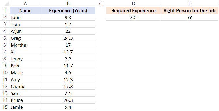
Example 8: Find the Closest Match
Let’s get a little advanced now.
Suppose you have a dataset where you want to find the person who has the work experience closest to the required experience (mentioned in cell D2).
While lookup formulas are not made to do this, you can combine it with other functions (such as MIN and ABS) to get this done.
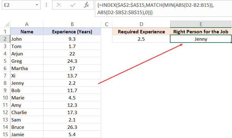
Below is the formula that will find the person with the experience closest to the required one and return the name of the person. Note that the experience needs to be closest (which can be either less or more).
=INDEX($A$2:$A$15,MATCH(MIN(ABS(D2-B2:B15)),ABS(D2-$B$2:$B$15),0))
Since this is an array formula, you need to use Control + Shift + Enter.
The trick in this formula is to change the lookup value and lookup array to find the minimum experience difference in required and actual values.
Before I explain the formula, let’s understand how you would do it manually.
You will go through each cell in column B and find the difference in the experience between what is required and the one that a person has. Once you have all the differences, you will find the one which is minimum and fetch the name of that person.
This is exactly what we are doing with this formula.
Let me explain.
The lookup value in the MATCH formula is MIN(ABS(D2-B2:B15)).
This part gives you the minimum difference between the given experience (which is 2.5 years) and all the other experiences. In this example, it returns 0.3
Note that I have used ABS to make sure I am looking for the closest (which can be more or less than the given experience).
Now, this minimum value becomes our lookup value.
The lookup array in the MATCH function is ABS(D2-$B$2:$B$15).
This gives us an array of numbers from which 2.5 (the required experience) has been subtracted.
So now we have a lookup value (0.3) and a lookup array ({6.8;0.8;19.5;21.8;14.5;11.2;0.3;9.2;2;9.8;14.8;0.4;23.8;2.9})
MATCH function finds the position of 0.3 in this array, which is also the position of the person’s name who has the closest experience.
This position number is then used by the INDEX function to return the name of the person.
Related Read: Find the Closest Match in Excel (examples using lookup formulas)
Click here to download the example file
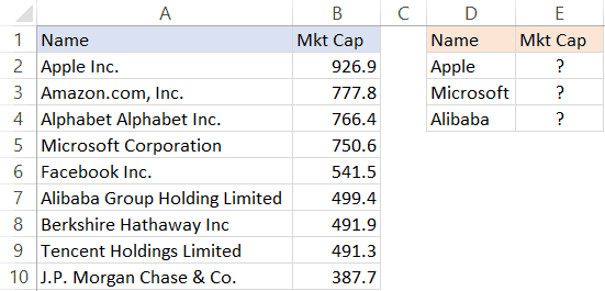
Example 9: Use INDEX MATCH with Wildcard Characters
If you want to look up a value when there is a partial match, then you need to use wildcard characters.
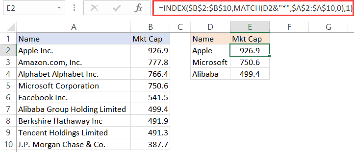
For example, below is a dataset of company name and their market capitalizations and you want to want to get the market cap. data for the three companies on the right.
Since these are not exact matches, you can’t do a regular lookup in this case.
But you can still get the right data by using an asterisk (*), which is a wildcard character.
Below is the formula that will give you the data by matching the company names from the main column and fetching the market cap figure for it.
=INDEX($B$2:$B$10,MATCH(D2&”*”,$A$2:$A$10,0),1)
Let me explain how this formula works.
Since there is no exact match of lookup values, I have used D2&”*” as the lookup value in the MATCH function.
An asterisk is a wildcard character that represents any number of characters. This means that Apple* in the formula would mean any text string that starts with the word Apple and can have any number of characters after it.
So when Apple* is used as the lookup value and the MATCH formula looks for it in column A, it returns the position of ‘Apple Inc.’, as it starts with the word Apple.
You can also use wildcard characters to find text strings where the lookup value is in between. For example, if you use *Apple* as the lookup value, it will find any string that has the word apple anywhere in it.
Note: This technique works well when you only have one instance of matching. But if you have multiple instances of matching (for example Apple Inc and Apple Corporation, then the MATCH function would return the position of the first matching instance only.
Example 10: Three Way Lookup
This is an advanced use of INDEX MATCH, but I will still cover it to show you the power of this combination.
Remember I said that INDEX function has two syntaxes:
=INDEX (array, row_num, [col_num])
=INDEX (array, row_num, [col_num], [area_num])
So far in all our examples, we have only used the first one.
But for a three-way lookup, you need to use the second syntax.
Let me first explain what a three-way look means.
In a two-way lookup, we use the INDEX MATCH formula to get the marks when we have the student’s name and the subject name. For example, fetching the marks of Jim in Math is a two-way lookup.
A three-way look would add another dimension to it. For example, suppose you have a dataset as shown below and you want to know the score of Jim in Math in Mid-term exam, then this would be three-way lookup.
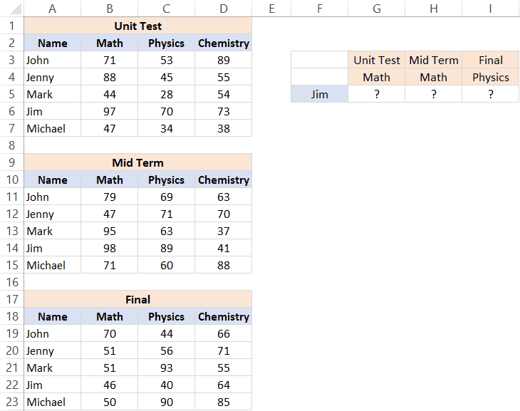
Below is the formula that will give the result.
=INDEX(($B$3:$D$7,$B$11:$D$15,$B$19:$D$23),MATCH($F$5,$A$3:$A$7,0),MATCH(G$4,$B$2:$D$2,0),(IF(G$3="Unit Test",1,IF(G$3="Mid Term",2,3))))
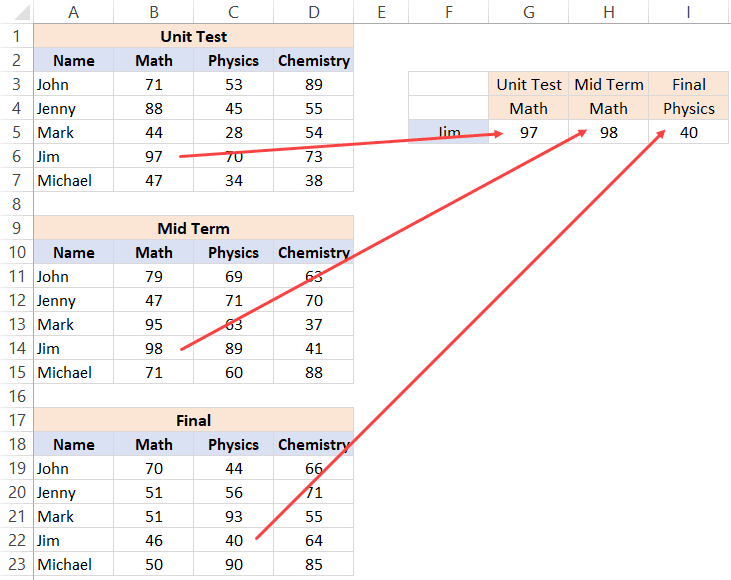
The above formula checked for three things – the name of the student, the subject, and the exam. After it finds the right value, it returns it in the cell.
Let me explain how this formula works by breaking down the formula into parts.
- array – ($B$3:$D$7,$B$11:$D$15,$B$19:$D$23): Instead of using a single array, in this case, I have used three arrays within parenthesis.
- row_num – MATCH($F$5,$A$3:$A$7,0): MATCH function is used to find the position of the student’s name in cell $F$5 in the list of student’s name.
- col_num – MATCH(G$4,$B$2:$D$2,0): MATCH function is used to find the position of the subject name in cell $B$2 in the list of subject’s name.
- [area_num] – IF(G$3=”Unit Test”,1,IF(G$3=”Mid Term”,2,3)): The area number value tells the INDEX function which of the three arrays to use to fetch the value. If the exam is Unit Term, the IF function would return 1 and the INDEX function would use the first array to fetch the value. If the exam is Mid-term, the IF formula would return 2, else it will return 3.
This is an advanced example of using INDEX MATCH, and you’re unlikely to find a situation when you have to use this. But it’s still good to know what Excel formulas can do.
Click here to download the example file
Why is INDEX/MATCH Better than VLOOKUP?
OR Is it?
Yes, it is – in most cases.
I will present my case in a while.
But before I do that, let me say this – VLOOKUP is an extremely useful function and I love it. It can do a lot of things in Excel and I use it every now and then myself. Having said that, it doesn’t mean that there can’t be anything better, and INDEX/MATCH (with more flexibility and functionalities) is better.
So if you want to do some basic lookup, you’re better off using VLOOKUP.
INDEX/MATCH is VLOOKUP on steroids. And once you learn INDEX/MATCH, you might always prefer using it (especially because of the flexibility it has).
Without stretching it too far, let me quickly give you the reasons why INDEX/MATCH is better than VLOOKUP.
INDEX/MATCH can look to the Left (as well as to the right) of the lookup value
I covered it in one of the example above.
If you have a value which is on the left of the lookup value, you can’t do that with VLOOKUP
At least not with just VLOOKUP.
Yes, you can combine VLOOKUP with other formulas and get it done, but it gets complicated and messy.
INDEX/MATCH, on the other hand, is made to lookup everywhere (be it left, right, up, or down)
INDEX/MATCH can work with vertical and horizontal ranges
Again, with full respect to VLOOKUP, it’s not made to do this.
After all, the V in VLOOKUP stands for vertical.
VLOOKUP can only go through data that is vertical, while INDEX/MATCH can go through data vertically as well horizontally.
Of course, there is the HLOOKUP function to take care of horizontal lookup, but it isn’t VLOOKUP then.. right?
I like the fact that INDEX MATCH combo is flexible enough to work with both vertical and horizontal data.
VLOOKUP cannot work with descending data
When it comes to the approximate match, VLOOKUP and INDEX/MATCH are at the same level.
But INDEX MATCH takes the point as it can also handle data that is in descending order.
I show this in one of the examples in this tutorial where we have to find the grade of students based on the grading table. If the table is sorted in descending order, VLOOKUP would not work (but INDEX MATCH would).
INDEX/MATCH can be slightly faster
I will be truthful. I didn’t run this test myself.
I am relying on the wisdom an Excel master – Charley Kyd.
The difference in speed in VLOOKUP and INDEX/MATCH is hardly noticeable when you have small data sets. But if you have thousands of rows and many columns, this can be a deciding factor.
In his article, Charley Kyd states:
“At its worst, the INDEX-MATCH method is about as fast as VLOOKUP; at its best, it’s much faster.”
INDEX/MATCH is Independent of the Actual Column Position
If you have a dataset as shown below as you’re fetching the score of Jim in Physics, you can do that using VLOOKUP.
And to do that, you can specify the column number as 3 in VLOOKUP.
All is fine.
But what if I delete the Math column.
In that case, the VLOOKUP formula will break.
Why? – Because it was hardcoded to use the third column, and when I delete a column in between, the third column becomes the second column.
Using INDEX/MATCH, in this case, is better as you can make the column number dynamic by using MATCH. So instead of a column number, it checks for the subject name and uses that to return the column number.
Surely you can do that by combining VLOOKUP with MATCH, but if you combining anyway, why not do it with INDEX which is a lot more flexible.
When using INDEX/MATCH, you can safely insert/delete columns in your dataset.
Despite all these factors, there is a reason VLOOKUP is so popular.
And it’s a big reason.
VLOOKUP is easier to use
VLOOKUP only takes a maximum of four arguments. If you can wrap your head around these four, you’re good to go.
And since most of the basic lookup cases are handled by VLOOKUP as well, it has quickly become the most popular Excel function.
I call it the King of Excel functions.
INDEX/MATCH, on the other hand, is a little more difficult to use. You may get a hang if it when you start using it, but for a beginner, VLOOKUP is far more easy to explain and learn.
And this is not a zero-sum game.
So, if you’re new to the lookup world and don’t know how to use VLOOKUP, better learn that.
I have a detailed guide on using VLOOKUP in Excel (with lots of examples)
My intent in this article is not to pitch two awesome functions against each other. I wanted to show you the power of INDEX MATCH combo and all the great things it can do.
Hope you found this article useful.
Let me know your thoughts in the comments section, and in case you find any mistake in this tutorial, please let me know.
You May Also Like the Following Excel Tutorials:
- Excel Functions
- 100+ Excel Interview Questions
- Find the Last Occurrnece of a Lookup Value in a List
- Lookup the Second, the Third, or the Nth Value in Excel
- Use IFERROR with VLOOKUP to Get Rid of #N/A Errors
Author: Oscar Cronquist Article last updated on November 08, 2021
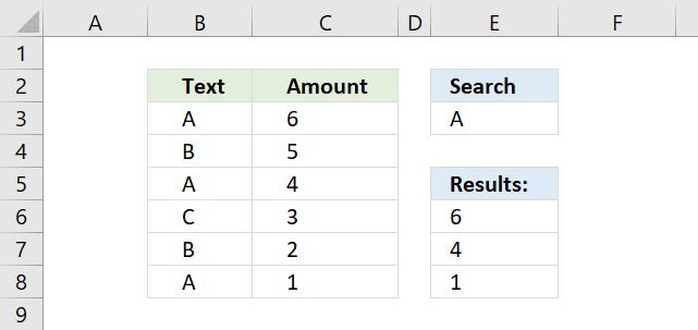
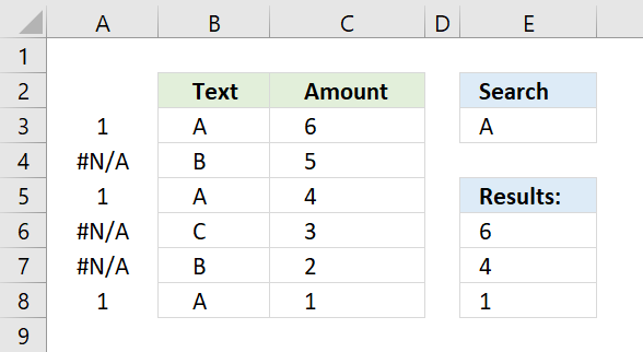
This article demonstrates how to use INDEX and MATCH functions to lookup and return multiple results. The lookup value is in cell E3, the lookup range is B3:B8.
Cells B3, B5, and B8 contains the lookup value, cell values in the corresponding cells in column C are returned. They are C3, C5, and C8.
There is actually a smaller formula that does the same thing: VLOOKUP — Return multiple values I also recommend the FILTER function if you are an Excel 365 user, the FILTER function is really easy to use.
The array formula in cell E6 extracts values from column C when the corresponding value in column B matches the value in cell E3.
The matching rows are 3, 5 and 8 so the array formula returns 3 values in cell range E6:E8.
=INDEX($C$3:$C$8, SMALL(IF(ISNUMBER(MATCH($B$3:$B$8, $E$3, 0)), MATCH(ROW($B$3:$B$8), ROW($B$3:$B$8)), «»), ROWS($A$1:A1)))
The formula above is an array formula, make sure you follow the instructions below on how to enter an array formula to make it work.
1. How to enter an array formula
To enter an array formula, type the formula in a cell then press and hold CTRL + SHIFT simultaneously, now press Enter once. Release all keys.
The formula bar now shows the formula enclosed with curly brackets telling you that you entered the formula successfully. Don’t enter the curly brackets yourself.
Now copy cell E6 and paste to cells below as far as needed.
2. Explaining formula in cell E6
Step 1 — Find matching values
The MATCH function matches a cell range against a single value returning an array.
MATCH($B$3:$B$8, $E$3, 0)
becomes
MATCH({«A»; «B»; «A»; «C»; «B»; «A»}, «A», 0)
and returns
{1; #N/A; 1; #N/A; #N/A; 1}.
If a value is equal to the search value MATCH function returns 1. If it is not equal the MATCH function returns #N/A.
The picture above displays the array in column A.
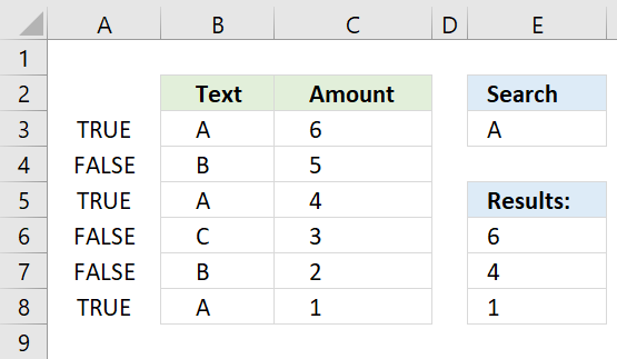
Step 2 — Convert array values to boolean values
The IF function cant process error values so to solve that I am going to use the ISNUMBER function to convert the array values to boolean values.
ISNUMBER(MATCH($B$3:$B$8, $E$3, 0))
becomes
ISNUMBER({1; #N/A; 1; #N/A; #N/A; 1})
and returns
{TRUE; FALSE; TRUE; FALSE; FALSE; TRUE}.
The array is shown in column A, see picture below.
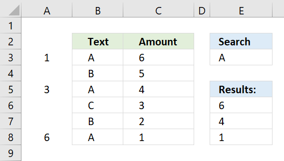
Step 3 — Identify rows
The IF function converts the boolean values into row numbers and blanks.
IF(ISNUMBER(MATCH($B$3:$B$8, $E$3, 0)), MATCH(ROW($B$3:$B$8), ROW($B$3:$B$8)), «»)
becomes
IF({TRUE; FALSE; TRUE; FALSE; FALSE; TRUE}, MATCH(ROW($B$3:$B$8), ROW($B$3:$B$8)), «»)
The MATCH and ROW functions calculate an array with sequential numbers, 1 to n, determined by the size of the cell range. In this case, $B$3:$B$8 has 6 values so the array becomes 1 to 6.
IF({TRUE; FALSE; TRUE; FALSE; FALSE; TRUE}, {1; 2; 3 ;4; 5; 6}, «»)
and returns
{1;»»;3;»»;»»;6}.
The picture below shows the relative row numbers for cell range B3:B8.
Step 4 — Get the k-th smallest row number
To be able to return the correct value the formula must know which value to get. The SMALL function determines the value to get based on row number.
SMALL(IF(ISNUMBER(MATCH($B$3:$B$8, $E$3, 0)), MATCH(ROW($B$3:$B$8), ROW($B$3:$B$8)), «»), ROWS($A$1:A1))
becomes
SMALL({1;»»;3;»»;»»;6}, ROWS($A$1:A1))
The ROWS function returns a number that changes when you copy the cell and paste to cells below.
SMALL({1;»»;3;»»;»»;6}, 1)
and returns 1.
In the next cell below ROWS($A$1:A1) changes to ROWS($A$1:A2) and returns 2.
Step 5 — Get values from column C using row numbers
The INDEX function returns a value from a given cell range based on a row and column number.
INDEX($C$3:$C$8, SMALL(IF(ISNUMBER(MATCH($B$3:$B$8, $E$3, 0)), MATCH(ROW($B$3:$B$8), ROW($B$3:$B$8)), «»), ROWS($A$1:A1)))
becomes
INDEX($C$3:$C$8, 1)
The first cell value in cell range $C$3:$C$8 is 6, the INDEX function returns 6 in cell E6.
3. Get Excel file
Related post
Recommended articles

Многие пользователи знают и применяют формулу ВПР. Известно также, что ВПР имеет ряд особенностей и ограничений, которые несложно обойти. Однако есть нюанс, который значительно ограничивает возможности функции ВПР.
ВПР требует, чтобы в диапазоне с искомыми данными столбец критериев всегда был первым слева. Это обстоятельство, конечно, является ограничением ВПР. Как же быть, если искомые данные находятся левее столбца с критерием? Можно, конечно, расположить столбцы в нужном порядке, что в целом, является неплохим выходом из ситуации. Но бывает так, что сделать этого нельзя, или трудно. К примеру, вы работаете в чужом документе или регулярно получаете новый отчет. В общем, нужно решение, не зависящее от расположения столбцов. Такое решение существует.
Нужно воспользоваться комбинацией из двух функций: ИНДЕКС и ПОИСКПОЗ. Формула работает следующим образом. ИНДЕКС отсчитывает необходимое количество ячеек вниз в диапазоне искомых значений. Количество отсчитываемых ячеек определяется по столбцу критериев функцией ПОИСКПОЗ. Работу комбинации этих функций удобно рассмотреть с середины, где вначале находится номер ячейки с подходящим критерием, а затем этот номер подставляется в ИНДЕКС.

Таким образом, чтобы подтянуть значение цены, соответствующее первому коду (книге), нужно прописать такую формулу.

Следует обратить внимание на корректность ссылок, чтобы при копировании формулы ничего не «съехало». Протягиваем формулу вниз. Если в таблице, откуда подтягиваются данные, нет искомого критерия, то функция выдает ошибку #Н/Д.

Довольно стандартная ситуация, с которой успешно справляется функция ЕСЛИОШИБКА. Она перехватывает ошибки и вместо них выдает что-либо другое, например, нули.
Конструкция формулы будет следующая:

Вот, собственно, и все.
Таким образом, комбинация функций ИНДЕКС и ПОИСКПОЗ является полной заменой ВПР и обладает дополнительным преимуществом: умеет находить данные слева от столбца с критерием. Кроме того, сами столбцы можно двигать как угодно, лишь бы ссылка не съехала, чего нельзя проделать с ВПР, т.к. количество столбцов там указывается конкретным числом. Посему комбинация ИНДЕКС и ПОИСКПОЗ более универсальна, чем ВПР.
Ниже видеоурок по работе функций ИНДЕКС и ПОИСКПОЗ.
Скачать файл с примером.
Поделиться в социальных сетях:
How to Use INDEX MATCH
With Multiple Criteria in Excel
INDEX MATCH with multiple criteria enables you to do a successful lookup when there are multiple lookup value matches.
In other words, you can look up and return values even if there are no unique values to look for.
This is not achievable with any other lookup formula without inserting helper columns😲
Follow these 3 easy steps to create your very own INDEX MATCH with multiple criteria in a few minutes.
If you want to tag along, download the sample Excel file here.
INDEX MATCH with multiple criteria example
So, you got this employee database.

You want to make the database easier to search, so you’re creating a small tool (to the right).
In that tool, anyone should be able to type in the name and division of an employee and it will find that person’s salary (and show it in cell G4).
“That’s easy, I can just use VLOOKUP.”
Wait a minute✋
Unfortunately, it’s not that easy.
You see, the problem is that there are actually 2 employees called “Steve Jones”. That means the lookup value has 2 matches in the lookup column.

There’s nothing unique about Steve Jones’ name on its own.
In Excel terminology, ‘Name’ would be 1 criteria.
So, 1 criteria didn’t cut it.
But if you include another criteria, like ‘Division’, you make Steve Jones unique.

Now, while “Steve Jones” appears several times on the list, there’s only one “Steve Jones from the sales division”.
This is the kind of magic you can do with INDEX MATCH with multiple criteria.
Step 1: Insert a normal INDEX MATCH formula
INDEX MATCH with multiple criteria is an ‘array formula’ created from the INDEX and MATCH functions.
An array formula has a syntax that is different from normal formulas. It’s basically a normal formula on steroids💪
The synergies between the INDEX and MATCH functions are that:
- MATCH searches for a value and returns a location
- MATCH feeds the location to the INDEX function
- Then INDEX transforms this location into a result

Start with:
=MATCH(
1. As the first argument in the MATCH function, enter the lookup value. This is what you are looking for.
In this case, you’re looking for an employee with the name “Steve Jones”.
Select (or manually enter) cell G2 as lookup value, then separate with a comma to move on to the lookup array.

2. The lookup array is the column where the MATCH function looks for the lookup value.
Select the column with the names, and then enter a comma to move on to the [match_type].

Now your formula should look like this:
=MATCH(G2,A:A,
3. A little drop-down list appears that gives you the choice between 1, 0, and -1.

The 0 option is the “exact match” option and is most commonly used. The -1 and 1 are similar to VLOOKUP’s “approximate match” method.
Write 0 or double-click the ‘0 – Exact match’ option in the drop-down menu and type the end parenthesis.

Your formula should now look like this:
=MATCH(G2,A:A,0)
4. Wrap the INDEX function around the MATCH function.

Your formula should look like this by now:
=INDEX(MATCH(G2,A:A,0)
But we’re not done yet✋
The syntax of the INDEX function goes:
INDEX(array, row number, column number)
The MATCH function should be the 2nd argument in the INDEX syntax.
Right now, it’s the 1st argument.
So, begin writing the real 1st argument: the array.
The INDEX array is the column you want to return values from.
The purpose of the multiple criteria INDEX MATCH is to find the salary of a specific employee.
So, the array is the salary column (column D).

Your formula should look like this by now:
=INDEX(D:D,MATCH(G2,A:A,0)
And just put an extra parenthesis at the end to wrap up the INDEX function.
So, the final formula looks like this:
=INDEX(D:D,MATCH(G2,A:A,0))
EXPLANATION
The MATCH function searches for the value in G2 (“Steve Jones”) in the database and then returns a number.
This number is the row in the data where the name “Steve Jones” is found.
This row number is then fed into the syntax of the INDEX function.
Problem: There’s more than one employee called “Steve Jones”. Whose salary are we actually seeing?
Excel lookup formulas always search from top to bottom, so you’re seeing the salary of the top Steve Jones (in row 3).
That’s the Steve you’re looking for.
But it’s dumb luck that you found him🍀
To make sure we always find Steve Jones from sales, follow the rest of the steps below.
Step 2: Change the lookup value to 1
Now, you need to change your normal INDEX MATCH formula into an array formula.
Sounds hard?
Don’t worry, I’ll guide you step-by-step😊
1. Change the lookup value of the MATCH function to 1. It’s just as easy as it sounds.

So, the formula changes from:
=INDEX(D:D,MATCH(G2,A:A,0))
To:
=INDEX(D:D,MATCH(1,A:A,0))
The “theory” behind this is not as simple as changing the lookup value.
Since you’re changing the formula from a normal one to an array formula, the structure of the formula changes a bit as well. By changing the lookup value to 1, you’re not actually telling the MATCH function to search for the number 1 in the lookup array (last name column).
In Excel-language, 1 means TRUE. 0 means FALSE.
When you enter our two criteria in the next step, the 1 in the MATCH function simply means:
“Look through the rows in the data and return the row number where all of the criteria are TRUE”.
If you wrote a zero, the formula would look for a row where all of our criteria are FALSE – and that wouldn’t really make sense.
Step 3: Write the criteria
The criteria replaces the 2nd argument of the MATCH function, with this structure:
(range=criteria1)*(range=criteria2)*(range=criteria3)*…
This way, you can have as many criteria as you need.
INDEX MATCH with 2 criteria
It’s typically enough to use 2 criteria to make your lookup value unique.
Criteria 1 = name
Criteria 2 = division
Let’s see if you can find “Steve Jones from sales” or if he’s lost in the woods🌳
Replace the structure above with the actual criteria:
(range=criteria1)*(range=criteria2)
(A:A=G2)*(B:B=G3)
A:A is the column with names. G2 is the name you’re looking for.
B:B is the column with division. G3 is the division you’re looking for.
Write that as the 2nd argument in the MATCH function, replacing what’s currently there.

Your formula should now look like this:
=INDEX(D:D,MATCH(1,(A:A=G2)*(B:B=G3),0))
It seems weird typing random parenthesis’ into formulas, but this is how you structure the criteria, so the array formula understands it.
If you’re using Microsoft 365 just press Enter and watch your beautiful multiple criteria lookup💡
Explanation: Ctrl + Shift + Enter
If you’re not using Microsoft 365, do not press Enter when you’re done with the formula. It won’t work.
Instead, press and hold Ctrl and Shift and then press Enter.
Warning: {curly brackets} will appear around your formula. They are supposed to be there!
Every time you make changes to this formula, you must end with Ctrl + Shift + Enter
(Instead of just regular “Enter” as you are probably used to)
That’s it – Now what?
Wow… You just learned how to use INDEX MATCH with multiple criteria…
It wasn’t so scary after all, right? 😎
Now, you’ve created a tool to easily look up employees and return their salary – even if there are multiple employees with the exact same name!
All fueled by the INDEX and MATCH functions.

Lookup formulas (and functions) in general are extremely useful and significantly speed up your work🏃
But multiple criteria lookups really save your day when the lookup value is not unique.
But if you really want to work more productively in Excel, you need to dive into macros.
Macros automate work processes, so you can do 50 things with just one click.
I promise you, it’s not as hard as you think.
Join my free 30-minute video course and get started with macros (for beginners).
Other relevant resources
INDEX MATCH is not the only lookup formula out there, although it’s the only one you can turn into an array formula. If you want to expand your toolbox you should definitely get to know VLOOKUP and the new XLOOKUP.
If you thought this was hard to understand, you should dive into the INDEX function and the MATCH function separately and get to know them better.
Another way to achieve a lookup with multiple criteria is with the good old Excel filter.
I hope this helps you!
Take care👋
Kasper Langmann2022-08-04T10:56:45+00:00
Page load link
How to combine INDEX, MATCH, and MATCH formulas in Excel as a lookup function
What is INDEX MATCH in Excel?
The INDEX MATCH[1] Formula is the combination of two functions in Excel: INDEX[2] and MATCH[3].
=INDEX() returns the value of a cell in a table based on the column and row number.
=MATCH() returns the position of a cell in a row or column.
Combined, the two formulas can look up and return the value of a cell in a table based on vertical and horizontal criteria. For short, this is referred to as just the Index Match function. To see a video tutorial, check out our free Excel Crash Course.
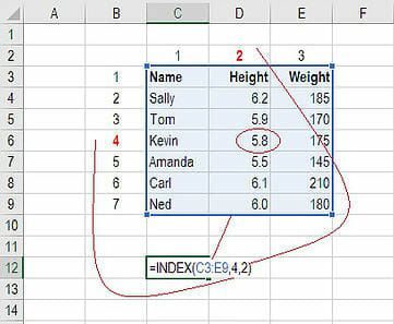
#1 How to Use the INDEX Formula
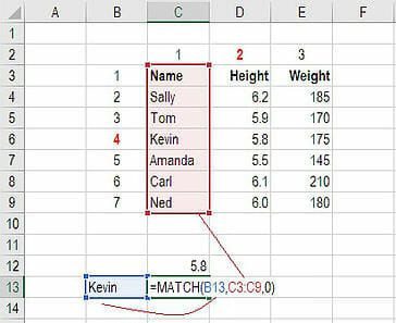
Below is a table showing people’s names, height, and weight. We want to use the INDEX formula to look up Kevin’s height… here is an example of how to do it.
Follow these steps:
- Type “=INDEX(” and select the area of the table, then add a comma
- Type the row number for Kevin, which is “4,” and add a comma
- Type the column number for Height, which is “2,” and close the bracket
- The result is “5.8.”
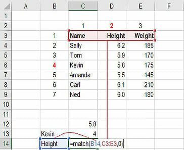
#2 How to Use the MATCH Formula
Sticking with the same example as above, let’s use MATCH to figure out what row Kevin is in.
Follow these steps:
- Type “=MATCH(” and link to the cell containing “Kevin”… the name we want to look up.
- Select all the cells in the Name column (including the “Name” header).
- Type zero “0” for an exact match.
- The result is that Kevin is in row “4.”
Use MATCH again to figure out what column Height is in.
Follow these steps:
- Type “=MATCH(” and link to the cell containing “Height”… the criteria we want to look up.
- Select all the cells across the top row of the table.
- Type zero “0” for an exact match.
- The result is that Height is in column “2.”
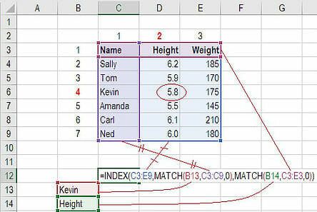
#3 How to Combine INDEX and MATCH
Now we can take the two MATCH formulas and use them to replace the “4” and the “2” in the original INDEX formula. The result is an INDEX MATCH formula.
Follow these steps:
- Cut the MATCH formula for Kevin and replace the “4” with it.
- Cut the MATCH formula for Height and replace the “2” with it.
- The result is Kevin’s Height is “5.8.”
- Congratulations, you now have a dynamic INDEX MATCH formula!
Video Explanation of How to Use Index Match in Excel
Below is a short video tutorial on how to combine the two functions and effectively use Index Match in Excel! Check out more free Excel tutorials on CFI’s YouTube Channel.
Hopefully, this short video made it even clearer how to use the two functions to dramatically improve your lookup capabilities in Excel.
More Excel Lessons
Thank you for reading this step-by-step guide to using INDEX MATCH in Excel. To continue learning and advancing your skills, these additional CFI resources will be helpful:
- Free Excel Fundamentals Course
- Excel Formulas and Functions List
- Excel Shortcuts
- Go To Special
- Find and Replace
- IF AND Function in Excel
- See all Excel resources
Функция INDEX (ИНДЕКС) в Excel используется для получения данных из таблицы, при условии что вы знаете номер строки и столбца, в котором эти данные находятся.
Например, в таблице ниже, вы можете использовать эту функцию для того, чтобы получить результаты экзамена по Физике у Андрея, зная номер строки и столбца, в которых эти данные находятся.

Содержание
- Что возвращает функция
- Синтаксис
- Аргументы функции
- Дополнительная информация
- Примеры использования функции ИНДЕКС в Excel
- Пример 1. Ищем результаты экзамена по физике для Алексея
- Пример 2. Создаем динамический поиск значений с использованием функций ИНДЕКС и ПОИСКПОЗ
- Пример 3. Создаем динамический поиск значений с использованием функций INDEX (ИНДЕКС) и MATCH (ПОИСКПОЗ) и выпадающего списка
- Пример 4. Использование трехстороннего поиска с помощью INDEX (ИНДЕКС) / MATCH (ПОИСКПОЗ)
Что возвращает функция
Возвращает данные из конкретной строки и столбца табличных данных.
Синтаксис
=INDEX (array, row_num, [col_num]) — английская версия
=INDEX (array, row_num, [col_num], [area_num]) — английская версия
=ИНДЕКС(массив; номер_строки; [номер_столбца]) — русская версия
=ИНДЕКС(ссылка; номер_строки; [номер_столбца]; [номер_области]) — русская версия
Аргументы функции
- array (массив) — диапазон ячеек или массив данных для поиска;
- row_num (номер_строки) — номер строки, в которой находятся искомые данные;
- [col_num] ([номер_столбца]) (необязательный аргумент) — номер колонки, в которой находятся искомые данные. Этот аргумент необязательный. Но если в аргументах функции не указаны критерии для row_num (номер_строки), необходимо указать аргумент col_num (номер_столбца);
- [area_num] ([номер_области]) — (необязательный аргумент) — если аргумент массива состоит из нескольких диапазонов, то это число будет использоваться для выбора всех диапазонов.
Дополнительная информация
- Если номер строки или колонки равен “0”, то функция возвращает данные всей строки или колонки;
- Если функция используется перед ссылкой на ячейку (например, A1), она возвращает ссылку на ячейку вместо значения (см. примеры ниже);
- Чаще всего INDEX (ИНДЕКС) используется совместно с функцией MATCH (ПОИСКПОЗ);
- В отличие от функции VLOOKUP (ВПР), функция INDEX (ИНДЕКС) может возвращать данные как справа от искомого значения, так и слева;
- Функция используется в двух формах — Массива данных и Формы ссылки на данные:
— Форма «Массива» используется когда вы хотите найти значения, основанные на конкретных номерах строк и столбцов таблицы;
— Форма «Ссылок на данные» используется при поиске значений в нескольких таблицах (используете аргумент [area_num] ([номер_области]) для выбора таблицы и только потом сориентируете функцию по номеру строки и столбца.
Примеры использования функции ИНДЕКС в Excel
Пример 1. Ищем результаты экзамена по физике для Алексея
Предположим, у вас есть результаты экзаменов в табличном виде по нескольким студентам:
Для того, чтобы найти результаты экзамена по физике для Андрея нам нужна формула:
=INDEX($B$3:$E$9,3,2) — английская версия
=ИНДЕКС($B$3:$E$9;3;2) — русская версия
В формуле мы определили аргумент диапазона данных, где мы будем искать данные $B$3:$E$9. Затем, указали номер строки “3”, в которой находятся результаты экзамена для Андрея, и номер колонки “2”, где находятся результаты экзамена именно по физике.
Пример 2. Создаем динамический поиск значений с использованием функций ИНДЕКС и ПОИСКПОЗ
Не всегда есть возможность указать номера строки и столбца вручную. У вас может быть огромная таблица данных, отображение данных которой вы можете сделать динамическим, чтобы функция автоматически идентифицировала имя или экзамен, указанные в ячейках, и дала правильный результат.
Пример динамического отображения данных ниже:

Для динамического отображения данных мы используем комбинацию функций INDEX (ИНДЕКС) и MATCH (ПОИСКПОЗ).
Вот такая формула поможет нам добиться результата:
=INDEX($B$3:$E$9,MATCH($G$4,$A$3:$A$9,0),MATCH($H$3,$B$2:$E$2,0)) — английская версия
=ИНДЕКС($B$3:$E$9;ПОИСКПОЗ($G$4;$A$3:$A$9;0);ПОИСКПОЗ($H$3;$B$2:$E$2;0)) — русская версия
В формуле выше, не используя сложного программирования, мы с помощью функции MATCH (ПОИСКПОЗ) сделали отображение данных динамическим.
Динамический отображение строки задается следующей частью формулы —
MATCH($G$4,$A$3:$A$9,0) — английская версия
ПОИСКПОЗ($G$4;$A$3:$A$9;0) — русская версия
Она сканирует имена студентов и определяет значение поиска ($G$4 в нашем случае). Затем она возвращает номер строки для поиска в наборе данных. Например, если значение поиска равно Алексей, функция вернет “1”, если это Максим, оно вернет “4” и так далее.
Динамическое отображение данных столбца задается следующей частью формулы —
MATCH($H$3,$B$2:$E$2,0) — английская версия
ПОИСКПОЗ($H$3;$B$2:$E$2;0) — русская версия
Она сканирует имена объектов и определяет значение поиска ($H$3 в нашем случае). Затем она возвращает номер столбца для поиска в наборе данных. Например, если значение поиска Математика, функция вернет “1”, если это Физика, функция вернет “2” и так далее.
Больше лайфхаков в нашем Telegram Подписаться
Пример 3. Создаем динамический поиск значений с использованием функций INDEX (ИНДЕКС) и MATCH (ПОИСКПОЗ) и выпадающего списка
На примере выше мы вручную вводили имена студентов и названия предметов. Вы можете сэкономить время на вводе данных, используя выпадающие списки. Это актуально, когда количество данных огромное.
Используя выпадающие списки, вам нужно просто выбрать из списка имя студента и функция автоматически найдет и подставит необходимые данные.
Пример ниже:

Используя такой подход, вы можете создать удобный дашборд, например для учителя. Ему не придется заниматься фильтрацией данных или прокруткой листа со студентами, для того чтобы найти результаты экзамена конкретного студента, достаточно просто выбрать имя и результаты динамически отразятся в лаконичной и удобной форме.
Для того, чтобы осуществить динамическую подстановку данных с использованием функций INDEX (ИНДЕКС) и MATCH (ПОИСКПОЗ) и выпадающего списка, мы используем ту же формулу, что в Примере 2:
=INDEX($B$3:$E$9,MATCH($G$4,$A$3:$A$9,0),MATCH($H$3,$B$2:$E$2,0)) — английская версия
=ИНДЕКС($B$3:$E$9;ПОИСКПОЗ($G$4;$A$3:$A$9;0);ПОИСКПОЗ($H$3;$B$2:$E$2;0)) — русская версия
Единственное отличие, от Примера 2, мы на месте ввода имени и предмета создадим выпадающие списки:
- Выбираем ячейку, в которой мы хотим отобразить выпадающий список с именами студентов;
- Кликаем на вкладку “Data” => Data Tools => Data Validation;
- В окне Data Validation на вкладке “Settings” в подразделе Allow выбираем “List”;
- В качестве Source нам нужно выбрать диапазон ячеек, в котором указаны имена студентов;
- Кликаем ОК
Теперь у вас есть выпадающий список с именами студентов в ячейке G5. Таким же образом вы можете создать выпадающий список с предметами.
Пример 4. Использование трехстороннего поиска с помощью INDEX (ИНДЕКС) / MATCH (ПОИСКПОЗ)
Функция INDEX (ИНДЕКС) может быть использована для обработки трехсторонних запросов.
Что такое трехсторонний поиск?
В приведенных выше примерах мы использовали одну таблицу с оценками для студентов по разным предметам. Это пример двунаправленного поиска, поскольку мы используем две переменные для получения оценки (имя студента и предмет).
Теперь предположим, что к концу года студент прошел три уровня экзаменов: «Вступительный», «Полугодовой» и «Итоговый экзамен».
Трехсторонний поиск — это возможность получить отметки студента по заданному предмету с указанным уровнем экзамена.
Вот пример трехстороннего поиска:
В приведенном выше примере, кроме выбора имени студента и названия предмета, вы также можете выбрать уровень экзамена. Основываясь на уровне экзамена, формула возвращает соответствующее значение из одной из трех таблиц.
Для таких расчетов нам поможет формула:
=INDEX(($B$3:$E$7,$B$11:$E$15,$B$19:$E$23),MATCH($G$4,$A$3:$A$7,0),MATCH($H$3,$B$2:$E$2,0),IF($H$2=»Вступительный»,1,IF($H$2=»Полугодовой»,2,3))) — английская версия
=ИНДЕКС(($B$3:$E$7;$B$11:$E$15;$B$19:$E$23);ПОИСКПОЗ($G$4;$A$3:$A$7;0);ПОИСКПОЗ($H$3;$B$2:$E$2;0); ЕСЛИ($H$2=»Вступительный»;1;ЕСЛИ($H$2=»Полугодовой»;2;3))) — русская версия
Давайте разберем эту формулу, чтобы понять, как она работает.
Эта формула принимает четыре аргумента. Функция INDEX (ИНДЕКС) — одна из тех функций в Excel, которая имеет более одного синтаксиса.
=INDEX (array, row_num, [col_num]) — английская версия
=INDEX (array, row_num, [col_num], [area_num]) — английская версия
=ИНДЕКС(массив; номер_строки; [номер_столбца]) — русская версия
=ИНДЕКС(ссылка; номер_строки; [номер_столбца]; [номер_области]) — русская версия
По всем вышеприведенным примерам мы использовали первый синтаксис, но для трехстороннего поиска нам нужно использовать второй синтаксис.
Рассмотрим каждую часть формулы на основе второго синтаксиса.
- array (массив) – ($B$3:$E$7,$B$11:$E$15,$B$19:$E$23):Вместо использования одного массива, в данном случае мы использовали три массива в круглых скобках.
- row_num (номер_строки) – MATCH($G$4,$A$3:$A$7,0): функция MATCH (ПОИСКПОЗ) используется для поиска имени студента для ячейки $G$4 из списка всех студентов.
- col_num (номер_столбца) – MATCH($H$3,$B$2:$E$2,0): функция MATCH (ПОИСКПОЗ) используется для поиска названия предмета для ячейки $H$3 из списка всех предметов.
- [area_num] ([номер_области]) – IF($H$2=”Вступительный”,1,IF($H$2=”Полугодовой”,2,3)): Значение номера области сообщает функции INDEX (ИНДЕКС), какой массив с данными выбрать. В этом примере у нас есть три массива в первом аргументе. Если вы выберете «Вступительный» из раскрывающегося меню, функция IF (ЕСЛИ) вернет значение “1”, а функция INDEX (ИНДЕКС) выберут 1-й массив из трех массивов ($B$3:$E$7).
Уверен, что теперь вы подробно изучили работу функции INDEX (ИНДЕКС) в Excel!