
This article explains in simple terms how to use INDEX and MATCH together to perform lookups. It takes a step-by-step approach, first explaining INDEX, then MATCH, then showing you how to combine the two functions together to create a dynamic two-way lookup. There are more advanced examples further down the page.
INDEX function | MATCH function | INDEX and MATCH | 2-way lookup | Left lookup | Case-sensitive | Closest match | Multiple criteria | More examples
The INDEX Function
The INDEX function in Excel is fantastically flexible and powerful, and you’ll find it in a huge number of Excel formulas, especially advanced formulas. But what does INDEX actually do? In a nutshell, INDEX retrieves the value at a given location in a range. For example, let’s say you have a table of planets in our solar system (see below), and you want to get the name of the 4th planet, Mars, with a formula. You can use INDEX like this:
=INDEX(B3:B11,4)

INDEX returns the value in the 4th row of the range.
Video: How to look things up with INDEX
What if you want to get the diameter of Mars with INDEX? In that case, we can supply both a row number and a column number, and provide a larger range. The INDEX formula below uses the full range of data in B3:D11, with a row number of 4 and column number of 2:
=INDEX(B3:D11,4,2)

INDEX retrieves the value at row 4, column 2.
To summarize, INDEX gets a value at a given location in a range of cells based on numeric position. When the range is one-dimensional, you only need to supply a row number. When the range is two-dimensional, you’ll need to supply both the row and column number.
At this point, you may be thinking «So what? How often do you actually know the position of something in a spreadsheet?»
Exactly right. We need a way to locate the position of things we’re looking for.
Enter the MATCH function.
The MATCH function
The MATCH function is designed for one purpose: find the position of an item in a range. For example, we can use MATCH to get the position of the word «peach» in this list of fruits like this:
=MATCH("peach",B3:B9,0)

MATCH returns 3, since «Peach» is the 3rd item. MATCH is not case-sensitive.
MATCH doesn’t care if a range is horizontal or vertical, as you can see below:
=MATCH("peach",C4:I4,0)

Same result with a horizontal range, MATCH returns 3.
Video: How to use MATCH for exact matches
Important: The last argument in the MATCH function is match_type. Match_type is important and controls whether matching is exact or approximate. In many cases you will want to use zero (0) to force exact match behavior. Match_type defaults to 1, which means approximate match, so it’s important to provide a value. See the MATCH page for more details.
INDEX and MATCH together
Now that we’ve covered the basics of INDEX and MATCH, how do we combine the two functions in a single formula? Consider the data below, a table showing a list of salespeople and monthly sales numbers for three months: January, February, and March.

Let’s say we want to write a formula that returns the sales number for February for a given salesperson. From the discussion above, we know we can give INDEX a row and column number to retrieve a value. For example, to return the February sales number for Frantz, we provide the range C3:E11 with a row 5 and column 2:
=INDEX(C3:E11,5,2) // returns $5194
But we obviously don’t want to hardcode numbers. Instead, we want a dynamic lookup.
How will we do that? The MATCH function of course. MATCH will work perfectly for finding the positions we need. Working one step at a time, let’s leave the column hardcoded as 2 and make the row number dynamic. Here’s the revised formula, with the MATCH function nested inside INDEX in place of 5:
=INDEX(C3:E11,MATCH("Frantz",B3:B11,0),2)
Taking things one step further, we’ll use the value from H2 in MATCH:
=INDEX(C3:E11,MATCH(H2,B3:B11,0),2)

MATCH finds «Frantz» and returns 5 to INDEX for row.
To summarize:
- INDEX needs numeric positions.
- MATCH finds those positions.
- MATCH is nested inside INDEX.
Let’s now tackle the column number.
Two-way lookup with INDEX and MATCH
Above, we used the MATCH function to find the row number dynamically, but hardcoded the column number. How can we make the formula fully dynamic, so we can return sales for any given salesperson in any given month? The trick is to use MATCH twice – once to get a row position, and once to get a column position.
From the examples above, we know MATCH works fine with both horizontal and vertical arrays. That means we can easily find the position of a given month with MATCH. For example, this formula returns the position of March, which is 3:
=MATCH("Mar",C2:E2,0) // returns 3
But of course we don’t want to hardcode any values, so let’s update the worksheet to allow the input of a month name, and use MATCH to find the column number we need. The screen below shows the result:

A fully dynamic, two-way lookup with INDEX and MATCH.
=INDEX(C3:E11,MATCH(H2,B3:B11,0),MATCH(H3,C2:E2,0))
The first MATCH formula returns 5 to INDEX as the row number, the second MATCH formula returns 3 to INDEX as the column number. Once MATCH runs, the formula simplifies to:
=INDEX(C3:E11,5,3)
and INDEX correctly returns $10,525, the sales number for Frantz in March.
Note: you could use Data Validation to create dropdown menus to select salesperson and month.
Video: How to do a two-way lookup with INDEX and MATCH
Video: How to debug a formula with F9 (to see MATCH return values)
Left lookup
One of the key advantages of INDEX and MATCH over the VLOOKUP function is the ability to perform a «left lookup». Simply put, this just means a lookup where the ID column is to the right of the values you want to retrieve, as seen in the example below:

Read a detailed explanation here.
Case-sensitive lookup
By itself, the MATCH function is not case-sensitive. However, you use the EXACT function with INDEX and MATCH to perform a lookup that respects upper and lower case, as shown below:

Read a detailed explanation here.
Note: this is an array formula and must be entered with control + shift + enter, except in Excel 365.
Closest match
Another example that shows off the flexibility of INDEX and MATCH is the problem of finding the closest match. In the example below, we use the MIN function together with the ABS function to create a lookup value and a lookup array inside the MATCH function. Essentially, we use MATCH to find the smallest difference. Then we use INDEX to retrieve the associated trip from column B.

Read a detailed explanation here.
Note: this is an array formula and must be entered with control + shift + enter, except in Excel 365.
Multiple criteria lookup
One of the trickiest problems in Excel is a lookup based on multiple criteria. In other words, a lookup that matches on more than one column at the same time. In the example below, we are using INDEX and MATCH and boolean logic to match on 3 columns: Item, Color, and Size:

Read a detailed explanation here. You can use this same approach with XLOOKUP.
Note: this is an array formula and must be entered with control + shift + enter, except in Excel 365.
More examples of INDEX + MATCH
Here are some more basic examples of INDEX and MATCH in action, each with a detailed explanation:
- Basic INDEX and MATCH exact (features Toy Story)
- Basic INDEX and MATCH approximate (grades)
- Two-way lookup with INDEX and MATCH (approximate match)
Tip: Try using the new XLOOKUP and XMATCH functions, improved versions of the functions described in this article. These new functions work in any direction and return exact matches by default, making them easier and more convenient to use than their predecessors.
Suppose that you have a list of office location numbers, and you need to know which employees are in each office. The spreadsheet is huge, so you might think it is challenging task. It’s actually quite easy to do with a lookup function.
The VLOOKUP and HLOOKUP functions, together with INDEX and MATCH, are some of the most useful functions in Excel.
Note: The Lookup Wizard feature is no longer available in Excel.
Here’s an example of how to use VLOOKUP.
=VLOOKUP(B2,C2:E7,3,TRUE)
In this example, B2 is the first argument—an element of data that the function needs to work. For VLOOKUP, this first argument is the value that you want to find. This argument can be a cell reference, or a fixed value such as «smith» or 21,000. The second argument is the range of cells, C2-:E7, in which to search for the value you want to find. The third argument is the column in that range of cells that contains the value that you seek.
The fourth argument is optional. Enter either TRUE or FALSE. If you enter TRUE, or leave the argument blank, the function returns an approximate match of the value you specify in the first argument. If you enter FALSE, the function will match the value provide by the first argument. In other words, leaving the fourth argument blank—or entering TRUE—gives you more flexibility.
This example shows you how the function works. When you enter a value in cell B2 (the first argument), VLOOKUP searches the cells in the range C2:E7 (2nd argument) and returns the closest approximate match from the third column in the range, column E (3rd argument).
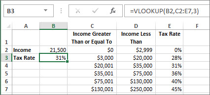
The fourth argument is empty, so the function returns an approximate match. If it didn’t, you’d have to enter one of the values in columns C or D to get a result at all.
When you’re comfortable with VLOOKUP, the HLOOKUP function is equally easy to use. You enter the same arguments, but it searches in rows instead of columns.
Using INDEX and MATCH instead of VLOOKUP
There are certain limitations with using VLOOKUP—the VLOOKUP function can only look up a value from left to right. This means that the column containing the value you look up should always be located to the left of the column containing the return value. Now if your spreadsheet isn’t built this way, then do not use VLOOKUP. Use the combination of INDEX and MATCH functions instead.
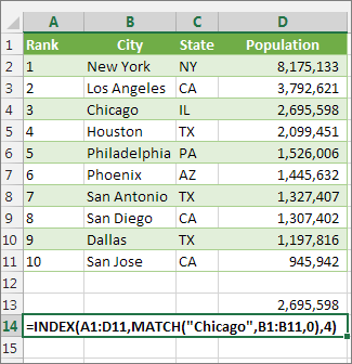
This example shows a small list where the value we want to search on, Chicago, isn’t in the leftmost column. So, we can’t use VLOOKUP. Instead, we’ll use the MATCH function to find Chicago in the range B1:B11. It’s found in row 4. Then, INDEX uses that value as the lookup argument, and finds the population for Chicago in the 4th column (column D). The formula used is shown in cell A14.
For more examples of using INDEX and MATCH instead of VLOOKUP, see the article https://www.mrexcel.com/excel-tips/excel-vlookup-index-match/ by Bill Jelen, Microsoft MVP.
Give it a try
If you want to experiment with lookup functions before you try them out with your own data, here’s some sample data.
VLOOKUP Example at work
Copy the following data into a blank spreadsheet.
Tip: Before you paste the data into Excel, set the column widths for columns A through C to 250 pixels, and click Wrap Text (Home tab, Alignment group).
|
Density |
Viscosity |
Temperature |
|
0.457 |
3.55 |
500 |
|
0.525 |
3.25 |
400 |
|
0.606 |
2.93 |
300 |
|
0.675 |
2.75 |
250 |
|
0.746 |
2.57 |
200 |
|
0.835 |
2.38 |
150 |
|
0.946 |
2.17 |
100 |
|
1.09 |
1.95 |
50 |
|
1.29 |
1.71 |
0 |
|
Formula |
Description |
Result |
|
=VLOOKUP(1,A2:C10,2) |
Using an approximate match, searches for the value 1 in column A, finds the largest value less than or equal to 1 in column A which is 0.946, and then returns the value from column B in the same row. |
2.17 |
|
=VLOOKUP(1,A2:C10,3,TRUE) |
Using an approximate match, searches for the value 1 in column A, finds the largest value less than or equal to 1 in column A, which is 0.946, and then returns the value from column C in the same row. |
100 |
|
=VLOOKUP(0.7,A2:C10,3,FALSE) |
Using an exact match, searches for the value 0.7 in column A. Because there is no exact match in column A, an error is returned. |
#N/A |
|
=VLOOKUP(0.1,A2:C10,2,TRUE) |
Using an approximate match, searches for the value 0.1 in column A. Because 0.1 is less than the smallest value in column A, an error is returned. |
#N/A |
|
=VLOOKUP(2,A2:C10,2,TRUE) |
Using an approximate match, searches for the value 2 in column A, finds the largest value less than or equal to 2 in column A, which is 1.29, and then returns the value from column B in the same row. |
1.71 |
HLOOKUP Example
Copy all the cells in this table and paste it into cell A1 on a blank worksheet in Excel.
Tip: Before you paste the data into Excel, set the column widths for columns A through C to 250 pixels, and click Wrap Text (Home tab, Alignment group).
|
Axles |
Bearings |
Bolts |
|
4 |
4 |
9 |
|
5 |
7 |
10 |
|
6 |
8 |
11 |
|
Formula |
Description |
Result |
|
=HLOOKUP(«Axles», A1:C4, 2, TRUE) |
Looks up «Axles» in row 1, and returns the value from row 2 that’s in the same column (column A). |
4 |
|
=HLOOKUP(«Bearings», A1:C4, 3, FALSE) |
Looks up «Bearings» in row 1, and returns the value from row 3 that’s in the same column (column B). |
7 |
|
=HLOOKUP(«B», A1:C4, 3, TRUE) |
Looks up «B» in row 1, and returns the value from row 3 that’s in the same column. Because an exact match for «B» is not found, the largest value in row 1 that is less than «B» is used: «Axles,» in column A. |
5 |
|
=HLOOKUP(«Bolts», A1:C4, 4) |
Looks up «Bolts» in row 1, and returns the value from row 4 that’s in the same column (column C). |
11 |
|
=HLOOKUP(3, {1,2,3;»a»,»b»,»c»;»d»,»e»,»f»}, 2, TRUE) |
Looks up the number 3 in the three-row array constant, and returns the value from row 2 in the same (in this case, third) column. There are three rows of values in the array constant, each row separated by a semicolon (;). Because «c» is found in row 2 and in the same column as 3, «c» is returned. |
c |
INDEX and MATCH Examples
This last example employs the INDEX and MATCH functions together to return the earliest invoice number and its corresponding date for each of five cities. Because the date is returned as a number, we use the TEXT function to format it as a date. The INDEX function actually uses the result of the MATCH function as its argument. The combination of the INDEX and MATCH functions are used twice in each formula – first, to return the invoice number, and then to return the date.
Copy all the cells in this table and paste it into cell A1 on a blank worksheet in Excel.
Tip: Before you paste the data into Excel, set the column widths for columns A through D to 250 pixels, and click Wrap Text (Home tab, Alignment group).
|
Invoice |
City |
Invoice Date |
Earliest invoice by city, with date |
|
3115 |
Atlanta |
4/7/12 |
=»Atlanta = «&INDEX($A$2:$C$33,MATCH(«Atlanta»,$B$2:$B$33,0),1)& «, Invoice date: » & TEXT(INDEX($A$2:$C$33,MATCH(«Atlanta»,$B$2:$B$33,0),3),»m/d/yy») |
|
3137 |
Atlanta |
4/9/12 |
=»Austin = «&INDEX($A$2:$C$33,MATCH(«Austin»,$B$2:$B$33,0),1)& «, Invoice date: » & TEXT(INDEX($A$2:$C$33,MATCH(«Austin»,$B$2:$B$33,0),3),»m/d/yy») |
|
3154 |
Atlanta |
4/11/12 |
=»Dallas = «&INDEX($A$2:$C$33,MATCH(«Dallas»,$B$2:$B$33,0),1)& «, Invoice date: » & TEXT(INDEX($A$2:$C$33,MATCH(«Dallas»,$B$2:$B$33,0),3),»m/d/yy») |
|
3191 |
Atlanta |
4/21/12 |
=»New Orleans = «&INDEX($A$2:$C$33,MATCH(«New Orleans»,$B$2:$B$33,0),1)& «, Invoice date: » & TEXT(INDEX($A$2:$C$33,MATCH(«New Orleans»,$B$2:$B$33,0),3),»m/d/yy») |
|
3293 |
Atlanta |
4/25/12 |
=»Tampa = «&INDEX($A$2:$C$33,MATCH(«Tampa»,$B$2:$B$33,0),1)& «, Invoice date: » & TEXT(INDEX($A$2:$C$33,MATCH(«Tampa»,$B$2:$B$33,0),3),»m/d/yy») |
|
3331 |
Atlanta |
4/27/12 |
|
|
3350 |
Atlanta |
4/28/12 |
|
|
3390 |
Atlanta |
5/1/12 |
|
|
3441 |
Atlanta |
5/2/12 |
|
|
3517 |
Atlanta |
5/8/12 |
|
|
3124 |
Austin |
4/9/12 |
|
|
3155 |
Austin |
4/11/12 |
|
|
3177 |
Austin |
4/19/12 |
|
|
3357 |
Austin |
4/28/12 |
|
|
3492 |
Austin |
5/6/12 |
|
|
3316 |
Dallas |
4/25/12 |
|
|
3346 |
Dallas |
4/28/12 |
|
|
3372 |
Dallas |
5/1/12 |
|
|
3414 |
Dallas |
5/1/12 |
|
|
3451 |
Dallas |
5/2/12 |
|
|
3467 |
Dallas |
5/2/12 |
|
|
3474 |
Dallas |
5/4/12 |
|
|
3490 |
Dallas |
5/5/12 |
|
|
3503 |
Dallas |
5/8/12 |
|
|
3151 |
New Orleans |
4/9/12 |
|
|
3438 |
New Orleans |
5/2/12 |
|
|
3471 |
New Orleans |
5/4/12 |
|
|
3160 |
Tampa |
4/18/12 |
|
|
3328 |
Tampa |
4/26/12 |
|
|
3368 |
Tampa |
4/29/12 |
|
|
3420 |
Tampa |
5/1/12 |
|
|
3501 |
Tampa |
5/6/12 |
How to combine INDEX, MATCH, and MATCH formulas in Excel as a lookup function
What is INDEX MATCH in Excel?
The INDEX MATCH[1] Formula is the combination of two functions in Excel: INDEX[2] and MATCH[3].
=INDEX() returns the value of a cell in a table based on the column and row number.
=MATCH() returns the position of a cell in a row or column.
Combined, the two formulas can look up and return the value of a cell in a table based on vertical and horizontal criteria. For short, this is referred to as just the Index Match function. To see a video tutorial, check out our free Excel Crash Course.
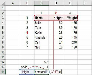
#1 How to Use the INDEX Formula
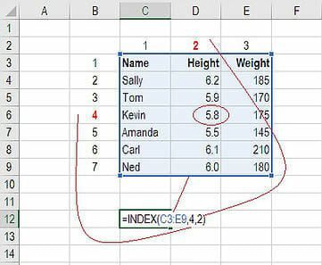
Below is a table showing people’s names, height, and weight. We want to use the INDEX formula to look up Kevin’s height… here is an example of how to do it.
Follow these steps:
- Type “=INDEX(” and select the area of the table, then add a comma
- Type the row number for Kevin, which is “4,” and add a comma
- Type the column number for Height, which is “2,” and close the bracket
- The result is “5.8.”
#2 How to Use the MATCH Formula
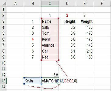
Sticking with the same example as above, let’s use MATCH to figure out what row Kevin is in.
Follow these steps:
- Type “=MATCH(” and link to the cell containing “Kevin”… the name we want to look up.
- Select all the cells in the Name column (including the “Name” header).
- Type zero “0” for an exact match.
- The result is that Kevin is in row “4.”
Use MATCH again to figure out what column Height is in.
Follow these steps:
- Type “=MATCH(” and link to the cell containing “Height”… the criteria we want to look up.
- Select all the cells across the top row of the table.
- Type zero “0” for an exact match.
- The result is that Height is in column “2.”
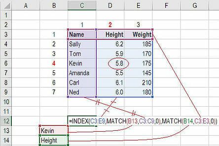
#3 How to Combine INDEX and MATCH
Now we can take the two MATCH formulas and use them to replace the “4” and the “2” in the original INDEX formula. The result is an INDEX MATCH formula.
Follow these steps:
- Cut the MATCH formula for Kevin and replace the “4” with it.
- Cut the MATCH formula for Height and replace the “2” with it.
- The result is Kevin’s Height is “5.8.”
- Congratulations, you now have a dynamic INDEX MATCH formula!
Video Explanation of How to Use Index Match in Excel
Below is a short video tutorial on how to combine the two functions and effectively use Index Match in Excel! Check out more free Excel tutorials on CFI’s YouTube Channel.
Hopefully, this short video made it even clearer how to use the two functions to dramatically improve your lookup capabilities in Excel.
More Excel Lessons
Thank you for reading this step-by-step guide to using INDEX MATCH in Excel. To continue learning and advancing your skills, these additional CFI resources will be helpful:
- Free Excel Fundamentals Course
- Excel Formulas and Functions List
- Excel Shortcuts
- Go To Special
- Find and Replace
- IF AND Function in Excel
- See all Excel resources
Excel has a lot of functions – about 450+ of them.
And many of these are simply awesome. The amount of work you can get done with a few formulas still surprises me (even after having used Excel for 10+ years).
And among all these amazing functions, the INDEX MATCH functions combo stands out.
I am a huge fan of INDEX MATCH combo and I have made it pretty clear many times.
I even wrote an article about Index Match Vs VLOOKUP which sparked a little bit of debate (you can check the comments section for some firework).
And today, I am writing this article solely focussed on Index Match to show you some simple and advanced scenarios where you can use this powerful formula combo and get the work done.
Note: There are other lookup formulas in Excel – such as VLOOKUP and HLOOKUP and these are great. Many people find VLOOKUP to be easier to use (and that’s true as well). I believe INDEX MATCH is a better option in many cases. But since people find it difficult, it gets used less. So I am trying to simplify it using this tutorial.
Now before I show you how the combination of INDEX MATCH is changing the world of analysts and data scientists, let me first introduce you to the individual parts – INDEX and MATCH functions.
INDEX Function: Finds the Value-Based on Coordinates
The easiest way to understand how Index function works is by thinking of it as a GPS satellite.
As soon as you tell the satellite the latitude and longitude coordinates, it will know exactly where to go and find that location.
So despite having a mind-boggling number of lat-long combinations, the satellite would know exactly where to look.
I quickly did a search for my work location and this is what I got.
Anyway, enough of geography.
Just like a satellite needs latitude and longitude coordinates, the INDEX function in Excel would need the row and column number to know what cell you’re referring to.
And that’s Excel INDEX function in a nut-shell.
So let me define it in simple words for you.
The INDEX function will use the row number and column number to find a cell in the given range and return the value in it.
All by itself, INDEX is a very simple function, with no utility. After all, in most cases, you are not likely to know the row and column numbers.
But…
The fact that you can use it with other functions (hint: MATCH) that can find the row number and the column number makes INDEX an extremely powerful Excel function.
Below is the syntax of the INDEX function:
=INDEX (array, row_num, [col_num])
=INDEX (array, row_num, [col_num], [area_num])
- array – a range of cells or an array constant.
- row_num – the row number from which the value is to be fetched.
- [col_num] – the column number from which the value is to be fetched. Although this is an optional argument, but if row_num is not provided, it needs to be given.
- [area_num] – (Optional) If array argument is made up of multiple ranges, this number would be used to select the reference from all the ranges.
INDEX function has 2 syntaxes (just FYI).
The first one is used in most cases. The second one is used in advanced cases only (such as doing a three-way lookup) which we will cover in one of the examples later in this tutorial.
But if you’re new to this function, just remember the first syntax.
Below is a video that explains how to use the INDEX function
MATCH Function: Finds the Position baed on a Lookup Value
Going back to my previous example of longitude and latitude, MATCH is the function that can find these positions (in the Excel spreadsheet world).
In simple language, the Excel MATCH function can find the position of a cell in a range.
And on what basis would it find a cell’s position?
Based on the lookup value.
For example, if you have a list as shown below and you want to find the position of the name ‘Mark’ in it, then you can use the MATCH function.
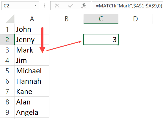
The function returns 3, as that’s the position of the cell with the name Mark in it.
MATCH function starts looking from top to bottom for the lookup value (which is ‘Mark’) in the specified range (which is A1:A9 in this example). As soon as it finds the name, it returns the position in that specific range.
Below is the syntax of the MATCH function in Excel.
=MATCH(lookup_value, lookup_array, [match_type])
- lookup_value – The value for which you are looking for a match in the lookup_array.
- lookup_array – The range of cells in which you are searching for the lookup_value.
- [match_type] – (Optional) This specifies how excel should look for a matching value. It can take three values -1, 0 , or 1.
Understanding Match Type Argument in MATCH Function
There is one additional thing you need to know about the MATCH function, and it’s about how it goes through the data and finds the cell position.
The third argument of the MATCH function can be 0, 1 or -1.
Below is an explanation of how these arguments work:
- 0 – this will look for an exact match of the value. If an exact match is found, the MATCH function will return the cell position. Else, it will return an error.
- 1 – this finds the largest value that is less than or equal to the lookup value. For this to work, your data range needs to be sorted in ascending order.
- -1 – this finds the smallest value that is greater than or equal to the lookup value. For this to work, your data range needs to be sorted in descending order.
Below is a video that explains how to use the MATCH function (along with the match type argument)
To summarize and put it in simple words:
- INDEX needs the cell position (row and column number) and gives the cell value.
- MATCH finds the position by using a lookup value.
Let’s Combine Them to Create a Powerhouse (INDEX + MATCH)
Now that you have a basic understanding of how INDEX and MATCH functions work individually, let’s combine these two and learn about all the wonderful things it can do.
To understand this better, I have a few examples that use the INDEX MATCH combination.
I will start with a simple example and then show you some advanced use cases as well.
Click here to download the example file
Example 1: A simple Lookup Using INDEX MATCH Combo
Let’s do a simple lookup with INDEX/MATCH.
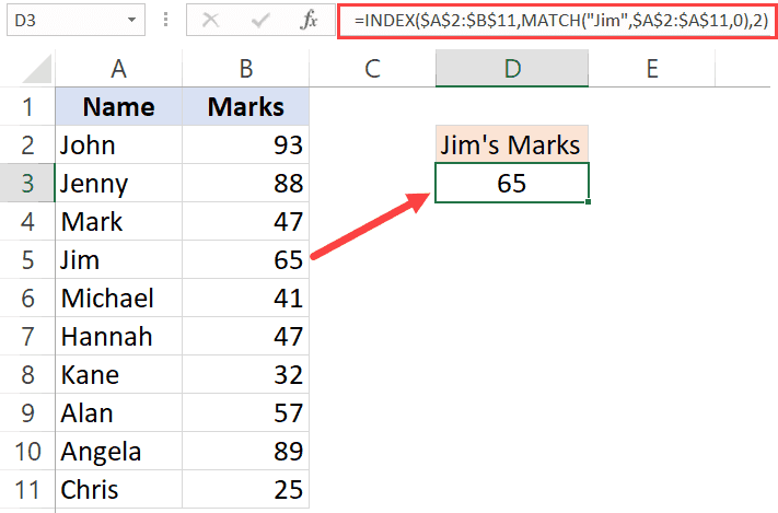
Below is a table where I have the marks for ten students.
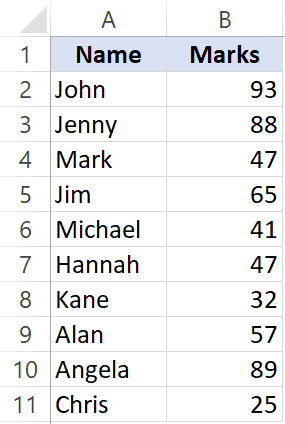
From this table, I want to find the marks for Jim.
Below is the formula that can easily do this:
=INDEX($A$2:$B$11,MATCH("Jim",$A$2:$A$11,0),2)
Now, if you’re thinking this can easily be done using a VLOOKUP function, you’re right! This is not the best use of INDEX MATCH awesomeness. Despite the fact that I am a fan of INDEX MATCH, it is a little more difficult than VLOOKUP. If fetching data from a column on the right is all you want to do, I recommend you use VLOOKUP.
The reason I have shown this example, which can also easily be done with VLOOKUP is to show you how INDEX MATCH works in a simple setting.
Now let me show a benefit of INDEX MATCH.
Suppose you have the same data, but instead of having it in columns, you have it in rows (as shown below).

You know what, you can still use INDEX MATCH combo to get Jim’s marks.
Below is the formula that will give you the result:
=INDEX($B$1:$K$2,2,MATCH(“Jim”,$B$1:$K$1,0))
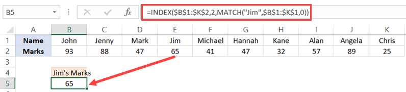
Note that you need to change the range and switch the row/column parts to make this formula work for horizontal data as well.
This can’t be done with VLOOKUP, but you can still do this easily with HLOOKUP.
INDEX MATCH combination can easily handle horizontal as well as vertical data.
Click here to download the example file
Example 2: Lookup to the Left
It’s more common than you think.
A lot of times, you may be required to fetch the data from a column which is to the left of the column that has the lookup value.
Something as shown below:
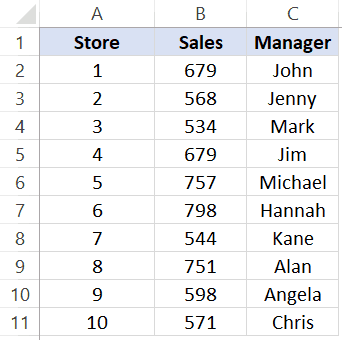
To find out Michael’s sales, you will have to do a lookup on the left.
If you’re thinking VLOOKUP, let me stop your right there.
VLOOKUP is not made to look for and fetch the values on the left.
Can you still do it using VLOOKUP?
Yes, you can!
But that can turn into a long and ugly formula.
So if you want to do a lookup and fetch data from the columns on the left, you are better off using INDEX MATCH combo.
Below is the formula that will get Michael’s sales number:
=INDEX($A$2:$C$11,MATCH("Michael",C2:C11,0),2)
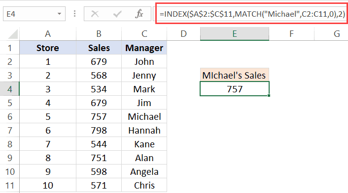
Another point here for INDEX MATCH. VLOOKUP can fetch the data only from the columns that are to the right of the column that has the lookup value.
Example 3: Two Way Lookup
So far, we have seen the examples where we wanted to fetch the data from the column adjacent to the column that has the lookup value.
But in real life, the data often spans through multiple columns.
INDEX MATCH can easily handle a two-way lookup.
Below is a dataset of the student’s marks in three different subjects.
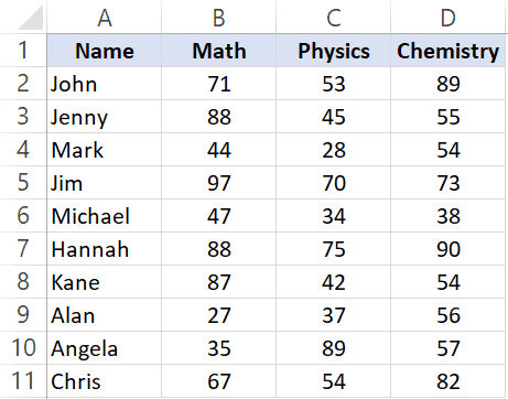
If you want to quickly fetch the marks of a student in all three subjects, you can do that with INDEX MATCH.
The below formula will give you the marks for Jim for all the three subjects (copy and paste in one cell and drag to fill other cells or copy and paste on other cells).
=INDEX($B$2:$D$11,MATCH($F$3,$A$2:$A$11,0),MATCH(G$2,$B$1:$D$1,0))

Let me quickly also explain this formula.
INDEX formula uses B2:D11 as the range.
The first MATCH uses the name (Jim in cell F3) and fetches the position of it in the names column (A2:A11). This becomes the row number from which the data needs to be fetched.
The second MATCH formula uses the subject name (in cell G2) to get the position of that specific subject name in B1:D1. For example, Math is 1, Physics is 2 and Chemistry is 3.
Since these MATCH positions are fed into the INDEX function, it returns the score based on the student name and subject name.
This formula is dynamic, which means that if you change the student name or the subject names, it would still work and fetch the correct data.
One great thing about using INDEX/MATCH is that even if you interchange the names of the subjects, it will continue to give you the correct result.
Example 4: Lookup Value From Multiple Column/Criteria
Suppose you have a dataset as shown below and you want to fetch the marks for ‘Mark Long’.

Since the data is in two columns, I can’t a lookup for Mark and get the data.
If I do it that way, I am going to get the marks data for Mark Frost and not Mark Long (because the MATCH function will give me the result for the MARK it meets).
One way of doing this is to create a helper column and combine the names. Once you have the helper column, you can use VLOOKUP and get the marks data.
If you’re interested in learning how to do this, read this tutorial on using VLOOKUP with multiple criteria.
But with INDEX/MATCH combo, you don’t need a helper column. You can create a formula that handles multiple criteria in the formula itself.
The below formula will give the result.
=INDEX($C$2:$C$11,MATCH($E$3&"|"&$F$3,$A$2:A11&"|"&$B$2:$B$11,0))

Let me quickly explain what this formula does.
The MATCH part of the formula combines the lookup value (Mark and Long) as well as the entire lookup array. When $A$2:A11&”|”&$B$2:$B$11 is used as the lookup array, it actually checks the lookup value against the combined string of first and last name (separated by the pipe symbol).
This ensures that you get the right result without using any helper columns.
You can do this kind of lookup (where there are multiple columns/criteria) with VLOOKUP as well, but you need to use a helper column. INDEX MATCH combo makes it slightly easy to do this without any helper columns.
Example 5: Get Values from Entire Row/Column
In the examples above, we have used the INDEX function to get value from a specific cell. You provide the row and column number, and it returns the value in that specific cell.
But you can do more.
You can also use the INDEX function to get the values from an entire row or column.
And how can this be useful you ask!
Suppose you want to know the total score of Jim in all the three subjects.
You can use the INDEX function to first get all the marks of Jim and then use the SUM function to get a total.
Let’s see how to do this.
Below I have the scores of all the students in three subjects.
The below formula will give me the total score of Jim in all the three subjects.
=SUM(INDEX($B$2:$D$11,MATCH($F$4,$A$2:$A$11,0),0))
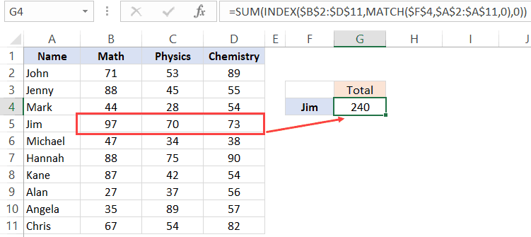
Let me explain how this formula works.
The trick here is to use 0 as the column number.
When you use 0 as the column number in the INDEX function, it will return all the row values. Similarly, if you use 0 as the row number, it will return all the values in the column.
So the below part of the formula returns an array of values – {97, 70, 73}
INDEX($B$2:$D$11,MATCH($F$4,$A$2:$A$11,0),0)
If you just enter this above formula in a cell in Excel and hit enter, you will see a #VALUE! error. This is because it’s not returning a single value, but an array of value.
But don’t worry, the array of values are still there. You can check this by selecting the formula and press the F9 key. It will show you the result of the formula which in this case is an array of three value – {97, 70, 73}
Now, if you wrap this INDEX formula in the SUM function, it will give you the sum of all the marks scored by Jim.
You can also use the same to get the highest, lowest and average marks of Jim.
Just like we have done this for a student, you can also do this for a subject. For example, if you want the average score in a subject, you can keep the row number as 0 in the INDEX formula and it will give you all the column values of that subject.
Click here to download the example file
Example 6: Find the Student’s Grade (Approximate Match Technique)
So far, we have used the MATCH formula to get the exact match of the lookup value.
But you can also use it to do an approximate match.
Now, what the hell is Approximate Match?
Let me explain.
When you’re looking for stuff such as names or ids, you’re looking for an exact match. But sometimes, you need to know the range in which your lookup values lie. This is usually the case with numbers.
For example, as a class teacher, you may want to know what’s the grade of each student in a subject, and the grade is decided based on the score.
Below is an example, where I want the grade for all the students and the grading is decided based on the table on the right.
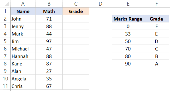
So if a student gets less than 33, the grade is F and if he/she gets less than 50 but more than 33, it’s E, and so on.
Below is the formula that will do this.
=INDEX($F$3:$F$8,MATCH(B2,$E$3:$E$8,1),1)
Let me explain how this formula works.
In the MATCH function, we have used 1 as the [match_type] argument. This argument will return the largest value that is less than or equal to the lookup value.
This means that the MATCH formula goes through the marks range, and as soon as it finds a marks range that is equal to or less than the lookup marks value, it will stop there and return its position.
So if the lookup mark value is 20, the MATCH function would return 1 and if it’s 85, it would return 5.
And the INDEX function uses this position value to get the grade.
IMPORTANT: For this to work, your data needs to be sorted in ascending order. If it’s not, you can get wrong results.
Note that the above can also be done using below VLOOKUP formula:
=VLOOKUP(B2,$E$3:$F$8,2,TRUE)
But MATCH function can go a step further when it comes to approximate match.
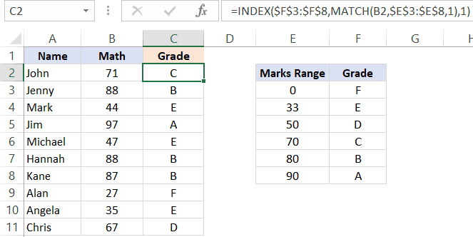
You can also have a descending data and can use INDEX MATCH combo to find the result. For example, if I change the order of the grade table (as shown below), I can still find the grades of the students.
To do this, all I have to do is change the [match_type] argument to -1.
Below is the formula that I have used:
=INDEX($F$3:$F$8,MATCH(B2,$E$3:$E$8,-1),1)
VLOOKUP can also do an approximate match but only when data is sorted in ascending order(but it doesn’t work if the data is sorted in descending order).
Example 7: Case Sensitive Lookups
So far all the lookups we have done have been case insensitive.
This means that whether the lookup value was Jim or JIM or jim, it didn’t matter. You’ll get the same result.
But what if you want the lookup to be case sensitive.
This is usually the case when you have large data sets and a possibility of repetition or distinct names/ids (with the only difference being the case)
For example, suppose I have the following data set of students where there are two students with the name Jim (the only difference being that one is entered as Jim and another one as jim).

Note that there are two students with the same name – Jim (cell A2 and A5).
Since a normal lookup wouldn’t work, you need to do a case sensitive lookup.
Below is the formula that will give you the right result. Since this is an array formula, you need to use Control + Shift + Enter.
=INDEX($B$2:$B$11,MATCH(TRUE,EXACT(D3,A2:A11),0),1)

Let me explain how this formula works.
The EXACT function checks for an exact match of the lookup value (which is ‘jim’ in this case). It goes through all the names and returns FALSE if it isn’t a match and TRUE if it’s a match.
So the output of the EXACT function in this example is – {FALSE;FALSE;FALSE;TRUE;FALSE;FALSE;FALSE;FALSE;FALSE;FALSE}
Note that there is only one TRUE, which is when the EXACT function found a perfect match.
The MATCH function then finds the position of TRUE in the array returned by the EXACT function, which is 4 in this example.
Once we have the position, the INDEX function uses it to find the marks.
Example 8: Find the Closest Match
Let’s get a little advanced now.
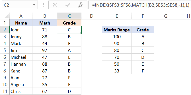
Suppose you have a dataset where you want to find the person who has the work experience closest to the required experience (mentioned in cell D2).
While lookup formulas are not made to do this, you can combine it with other functions (such as MIN and ABS) to get this done.
Below is the formula that will find the person with the experience closest to the required one and return the name of the person. Note that the experience needs to be closest (which can be either less or more).
=INDEX($A$2:$A$15,MATCH(MIN(ABS(D2-B2:B15)),ABS(D2-$B$2:$B$15),0))
Since this is an array formula, you need to use Control + Shift + Enter.
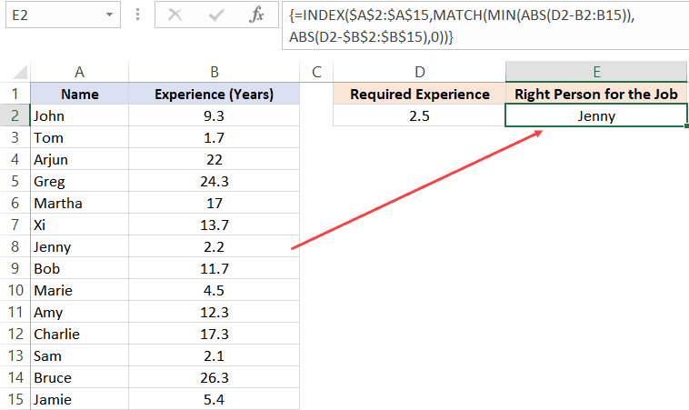
The trick in this formula is to change the lookup value and lookup array to find the minimum experience difference in required and actual values.
Before I explain the formula, let’s understand how you would do it manually.
You will go through each cell in column B and find the difference in the experience between what is required and the one that a person has. Once you have all the differences, you will find the one which is minimum and fetch the name of that person.
This is exactly what we are doing with this formula.
Let me explain.
The lookup value in the MATCH formula is MIN(ABS(D2-B2:B15)).
This part gives you the minimum difference between the given experience (which is 2.5 years) and all the other experiences. In this example, it returns 0.3
Note that I have used ABS to make sure I am looking for the closest (which can be more or less than the given experience).
Now, this minimum value becomes our lookup value.
The lookup array in the MATCH function is ABS(D2-$B$2:$B$15).
This gives us an array of numbers from which 2.5 (the required experience) has been subtracted.
So now we have a lookup value (0.3) and a lookup array ({6.8;0.8;19.5;21.8;14.5;11.2;0.3;9.2;2;9.8;14.8;0.4;23.8;2.9})
MATCH function finds the position of 0.3 in this array, which is also the position of the person’s name who has the closest experience.
This position number is then used by the INDEX function to return the name of the person.
Related Read: Find the Closest Match in Excel (examples using lookup formulas)
Click here to download the example file
Example 9: Use INDEX MATCH with Wildcard Characters
If you want to look up a value when there is a partial match, then you need to use wildcard characters.
For example, below is a dataset of company name and their market capitalizations and you want to want to get the market cap. data for the three companies on the right.
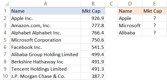
Since these are not exact matches, you can’t do a regular lookup in this case.
But you can still get the right data by using an asterisk (*), which is a wildcard character.
Below is the formula that will give you the data by matching the company names from the main column and fetching the market cap figure for it.
=INDEX($B$2:$B$10,MATCH(D2&”*”,$A$2:$A$10,0),1)
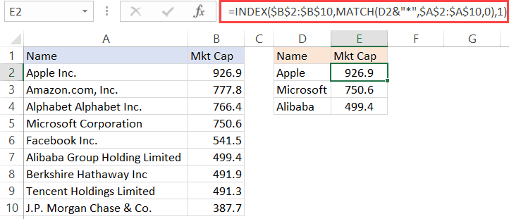
Let me explain how this formula works.
Since there is no exact match of lookup values, I have used D2&”*” as the lookup value in the MATCH function.
An asterisk is a wildcard character that represents any number of characters. This means that Apple* in the formula would mean any text string that starts with the word Apple and can have any number of characters after it.
So when Apple* is used as the lookup value and the MATCH formula looks for it in column A, it returns the position of ‘Apple Inc.’, as it starts with the word Apple.
You can also use wildcard characters to find text strings where the lookup value is in between. For example, if you use *Apple* as the lookup value, it will find any string that has the word apple anywhere in it.
Note: This technique works well when you only have one instance of matching. But if you have multiple instances of matching (for example Apple Inc and Apple Corporation, then the MATCH function would return the position of the first matching instance only.
Example 10: Three Way Lookup
This is an advanced use of INDEX MATCH, but I will still cover it to show you the power of this combination.
Remember I said that INDEX function has two syntaxes:
=INDEX (array, row_num, [col_num])
=INDEX (array, row_num, [col_num], [area_num])
So far in all our examples, we have only used the first one.
But for a three-way lookup, you need to use the second syntax.
Let me first explain what a three-way look means.
In a two-way lookup, we use the INDEX MATCH formula to get the marks when we have the student’s name and the subject name. For example, fetching the marks of Jim in Math is a two-way lookup.
A three-way look would add another dimension to it. For example, suppose you have a dataset as shown below and you want to know the score of Jim in Math in Mid-term exam, then this would be three-way lookup.
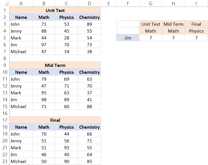
Below is the formula that will give the result.
=INDEX(($B$3:$D$7,$B$11:$D$15,$B$19:$D$23),MATCH($F$5,$A$3:$A$7,0),MATCH(G$4,$B$2:$D$2,0),(IF(G$3="Unit Test",1,IF(G$3="Mid Term",2,3))))
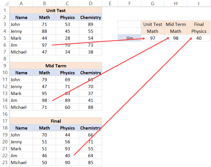
The above formula checked for three things – the name of the student, the subject, and the exam. After it finds the right value, it returns it in the cell.
Let me explain how this formula works by breaking down the formula into parts.
- array – ($B$3:$D$7,$B$11:$D$15,$B$19:$D$23): Instead of using a single array, in this case, I have used three arrays within parenthesis.
- row_num – MATCH($F$5,$A$3:$A$7,0): MATCH function is used to find the position of the student’s name in cell $F$5 in the list of student’s name.
- col_num – MATCH(G$4,$B$2:$D$2,0): MATCH function is used to find the position of the subject name in cell $B$2 in the list of subject’s name.
- [area_num] – IF(G$3=”Unit Test”,1,IF(G$3=”Mid Term”,2,3)): The area number value tells the INDEX function which of the three arrays to use to fetch the value. If the exam is Unit Term, the IF function would return 1 and the INDEX function would use the first array to fetch the value. If the exam is Mid-term, the IF formula would return 2, else it will return 3.
This is an advanced example of using INDEX MATCH, and you’re unlikely to find a situation when you have to use this. But it’s still good to know what Excel formulas can do.
Click here to download the example file
Why is INDEX/MATCH Better than VLOOKUP?
OR Is it?
Yes, it is – in most cases.
I will present my case in a while.
But before I do that, let me say this – VLOOKUP is an extremely useful function and I love it. It can do a lot of things in Excel and I use it every now and then myself. Having said that, it doesn’t mean that there can’t be anything better, and INDEX/MATCH (with more flexibility and functionalities) is better.
So if you want to do some basic lookup, you’re better off using VLOOKUP.
INDEX/MATCH is VLOOKUP on steroids. And once you learn INDEX/MATCH, you might always prefer using it (especially because of the flexibility it has).
Without stretching it too far, let me quickly give you the reasons why INDEX/MATCH is better than VLOOKUP.
INDEX/MATCH can look to the Left (as well as to the right) of the lookup value
I covered it in one of the example above.
If you have a value which is on the left of the lookup value, you can’t do that with VLOOKUP
At least not with just VLOOKUP.
Yes, you can combine VLOOKUP with other formulas and get it done, but it gets complicated and messy.
INDEX/MATCH, on the other hand, is made to lookup everywhere (be it left, right, up, or down)
INDEX/MATCH can work with vertical and horizontal ranges
Again, with full respect to VLOOKUP, it’s not made to do this.
After all, the V in VLOOKUP stands for vertical.
VLOOKUP can only go through data that is vertical, while INDEX/MATCH can go through data vertically as well horizontally.
Of course, there is the HLOOKUP function to take care of horizontal lookup, but it isn’t VLOOKUP then.. right?
I like the fact that INDEX MATCH combo is flexible enough to work with both vertical and horizontal data.
VLOOKUP cannot work with descending data
When it comes to the approximate match, VLOOKUP and INDEX/MATCH are at the same level.
But INDEX MATCH takes the point as it can also handle data that is in descending order.
I show this in one of the examples in this tutorial where we have to find the grade of students based on the grading table. If the table is sorted in descending order, VLOOKUP would not work (but INDEX MATCH would).
INDEX/MATCH can be slightly faster
I will be truthful. I didn’t run this test myself.
I am relying on the wisdom an Excel master – Charley Kyd.
The difference in speed in VLOOKUP and INDEX/MATCH is hardly noticeable when you have small data sets. But if you have thousands of rows and many columns, this can be a deciding factor.
In his article, Charley Kyd states:
“At its worst, the INDEX-MATCH method is about as fast as VLOOKUP; at its best, it’s much faster.”
INDEX/MATCH is Independent of the Actual Column Position
If you have a dataset as shown below as you’re fetching the score of Jim in Physics, you can do that using VLOOKUP.
And to do that, you can specify the column number as 3 in VLOOKUP.
All is fine.
But what if I delete the Math column.
In that case, the VLOOKUP formula will break.
Why? – Because it was hardcoded to use the third column, and when I delete a column in between, the third column becomes the second column.
Using INDEX/MATCH, in this case, is better as you can make the column number dynamic by using MATCH. So instead of a column number, it checks for the subject name and uses that to return the column number.
Surely you can do that by combining VLOOKUP with MATCH, but if you combining anyway, why not do it with INDEX which is a lot more flexible.
When using INDEX/MATCH, you can safely insert/delete columns in your dataset.
Despite all these factors, there is a reason VLOOKUP is so popular.
And it’s a big reason.
VLOOKUP is easier to use
VLOOKUP only takes a maximum of four arguments. If you can wrap your head around these four, you’re good to go.
And since most of the basic lookup cases are handled by VLOOKUP as well, it has quickly become the most popular Excel function.
I call it the King of Excel functions.
INDEX/MATCH, on the other hand, is a little more difficult to use. You may get a hang if it when you start using it, but for a beginner, VLOOKUP is far more easy to explain and learn.
And this is not a zero-sum game.
So, if you’re new to the lookup world and don’t know how to use VLOOKUP, better learn that.
I have a detailed guide on using VLOOKUP in Excel (with lots of examples)
My intent in this article is not to pitch two awesome functions against each other. I wanted to show you the power of INDEX MATCH combo and all the great things it can do.
Hope you found this article useful.
Let me know your thoughts in the comments section, and in case you find any mistake in this tutorial, please let me know.
You May Also Like the Following Excel Tutorials:
- Excel Functions
- 100+ Excel Interview Questions
- Find the Last Occurrnece of a Lookup Value in a List
- Lookup the Second, the Third, or the Nth Value in Excel
- Use IFERROR with VLOOKUP to Get Rid of #N/A Errors
INDEX-MATCH has become a more popular tool for Excel as it solves the limitation of the VLOOKUP function, and it is easier to use. INDEX-MATCH function in Excel has a number of advantages over the VLOOKUP function:
- INDEX and MATCH are more flexible and faster than Vlookup
- It is possible to execute horizontal lookup, vertical lookup, 2-way lookup, left lookup, case-sensitive lookup, and even lookups based on multiple criteria.
- In sorted Data, INDEX-MATCH is 30% faster than VLOOKUP. This means that in a larger dataset 30% faster makes more sense.
Let’s begin with the detailed concepts of each INDEX and MATCH.
INDEX Function
The INDEX function in Excel is very powerful at the same time a flexible tool that retrieves the value at a given location in a range. In another word, It returns the content of a cell, specified by row and column offset.
Syntax:
=INDEX(reference, [row], [column])
Parameters:
- reference: The array of cells to be offset into. It can be a single range or an entire dataset in a table of data.
- row [optional]: The number of offset rows. It means if we choose a table reference range as “A1:A5” then the Cell/content that we want to extract is at how much vertical distance. Here, for A1 row will be 1, for A2 row = 2, and so on. If we give row = 4 then it will extract A4. As row is optional so if we don’t specify any row number then it extracts entire rows in the reference range. That is A1 to A5 in this case.
- column [optional]: The number of offset columns. It means if we choose a table reference range as “A1:B5” then the Cell/content we want to extract is at how much horizontal distance. Here, for A1 row will be 1 and column will be 1, for B1 row will be 1 but the column will be 2 similarly for A2 row = 2 column = 1, for B2 row = 2 column = 2 and so on. If we give row = 5 and column 2 then it will extract B5. As the column is optional so if we don’t specify any row no. then it will extract the entire column in the reference range. For example, if we give row = 2 and column as empty then it will extract (A2:B2). If we don’t specify Row and column both then it will extract the entire reference table that is (A1:B5).
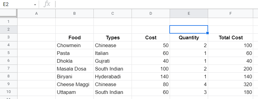
Reference Table: The following table will be used as a reference table for all the examples of the INDEX function. First Cell is at B3 (“FOOD”) and the Last Diagonal Cell is at F10 (“180”).
Examples: Below are some examples of Index functions.
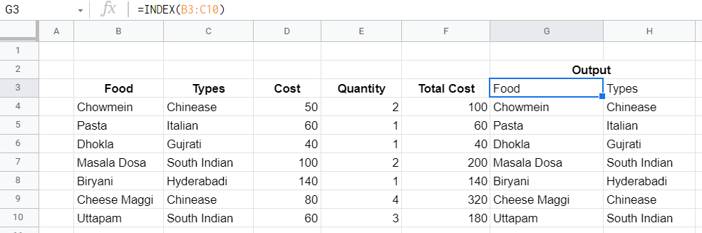
Case 1: No Rows and Columns are mentioned.
Input Command: =INDEX(B3:C10)
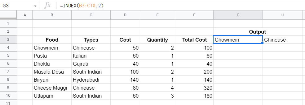
Case 2: Only Rows are Mentioned.
Input Command: =INDEX(B3:C10,2)
Case 3: Both Rows And Columns are mentioned.
Input Command: =INDEX(B3:D10,4,2)
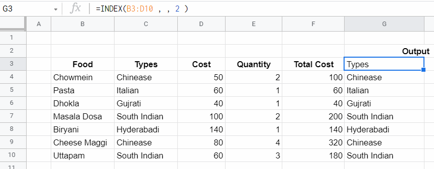
Case 4: Only Columns are mentioned.
Input Command: =INDEX(B3 : D10 , , 2)
Problem With INDEX Function: The problem with the INDEX function is that there is a need to specify rows and columns for the data that we are looking for. Let’s assume we are dealing with a machine learning dataset of 10000 rows and columns then it will be very difficult to search and extract the data that we are looking for. Here comes the concept of Match Function, which will identify rows and columns based on some condition.
MATCH Function
It retrieves the position of an item/value in a range. It is a less refined version of a VLOOKUP or HLOOKUP that only returns the location information and not the actual data. MATCH is not case-sensitive and does not care whether the range is Horizontal or Vertical.
Syntax:
=MATCH(search_key, range, [search_type])
Parameters:
- search_key: The value to search for. For example, 42, “Cats”, or I24.
- range: The one-dimensional array to be searched. It Can Either be a single row or a single column.eg->A1:A10 , A2:D2 etc.
- search_type [optional]: The search method. = 1 (default) finds the largest value less than or equal to search_key when the range is sorted in ascending order.
- = 0 finds the exact value when the range is unsorted.
- = -1 finds the smallest value greater than or equal to search_key when the range is sorted in descending order.
Row number or Column number can be found using the match function and can use it inside the index function so if there is any detail about an item, then all information can be extracted about the item by finding the row/column of the item using match then nesting it into index function.
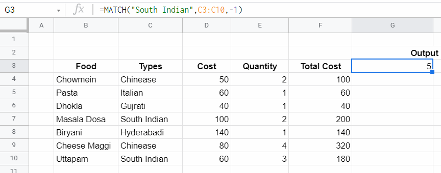
Reference Table: The following table will be used as a reference table for all the examples of the MATCH function. First Cell is at B3 (“FOOD”) and the Last Diagonal Cell is At F10 (“180”)
Examples: Below are some examples of the MATCH function-
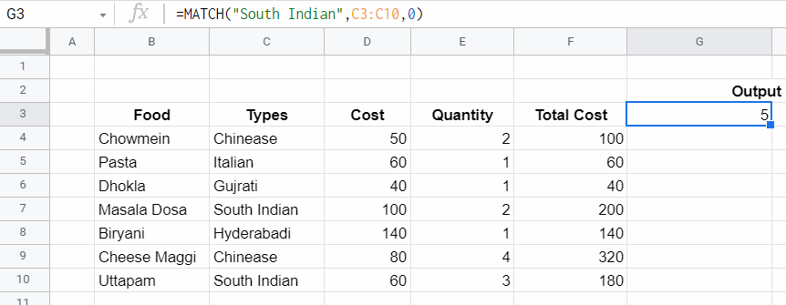
Case 1: Search Type 0, It means Exact Match.
Input Command: =MATCH(“South Indian”,C3:C10,0)
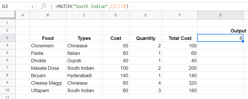
Case 2: Search Type 1 (Default).
Input Command: =MATCH(“South Indian”,C3:C10)
Case 3: Search Type -1.
Input Command: =MATCH(“South Indian”,C3:C10,-1)
INDEX-MATCH Together
In the previous examples, the static values of rows and columns were provided in the INDEX function Let’s assume there is no prior knowledge about the rows and column position then rows and columns position can be provided using the MATCH function. This Is a dynamic way to search and extract value.
Syntax:
=INDEX(Reference Table , [Match(SearchKey,Range,Type)/StaticRowPosition],
                         [Match(SearchKey,Range,Type)/StaticColumnPosition])
Reference Table: The following reference table will be used. First Cell is at B3 (“FOOD”) and the Last Diagonal Cell is At F10 (“180”)
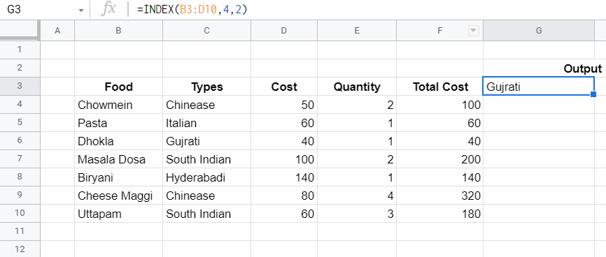
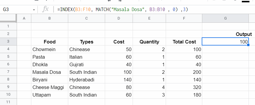
Example: Let’s say the task is to find the cost of Masala Dosa. It is known that column 3 represents the cost of items, but the row position of Masala Dosa is not known. The problem can be divided into two steps-
Step 1: Find the position of Masala Dosa by using the formula:
=MATCH("Masala Dosa",B3:B10,0)
Here B3:B10 represents Column “Food” and 0 means Exact Match. It will return the row number of Masala Dosa.
Step 2: Find the cost of Masala Dosa. Use the INDEX Function to find the cost of Masala Dosa. By substituting the above MATCH function query inside the INDEX function at the place where the exact position of Masala Dosa is required, and the column number of cost is 3 which is already known.
=INDEX(B3:F10, MATCH("Masala Dosa", B3:B10 , 0) ,3)
Two Ways Lookup With INDEX-MATCH Together
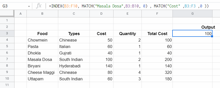
In the previous example, the column position Of the “Cost” attribute was hardcoded. So, It was not fully dynamic.
Case 1: Let’s assume there is no knowledge about the column number of Cost also, then it can be obtained using the formula:
=MATCH("Cost",B3:F3,0)
Here B3:F3 represents Header Column.
Case 2: When row, as well as column value, are provided via MATCH function (without giving static value) then it is called Two-Way Lookup. It can be achieved using the formula:
=INDEX(B3:F10, MATCH("Masala Dosa",B3:B10, 0) , MATCH("Cost" ,B3:F3 ,0))
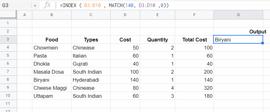
Left Lookup
One of the key advantages of INDEX and MATCH over the VLOOKUP function is the ability to perform a “left lookup”. It means it is possible to extract the row position of an item from using any attribute at right and the value of another attribute in left can be extracted.
For Example, Let’s say buy food whose cost should be 140 Rs. Indirectly we are saying buy “Biryani”. In this example, the cost Rs 140/- is known, there is a need to extract the “Food”. Since the Cost column is placed to the right of the Food column. If VLOOKUP is applied it will not be able to search the left side of the Cost column. That is why using VLOOKUP it is not possible to get Food Name.
To overcome this disadvantage INDEX-MATCH function Left lookup can be used.
Step 1: First extract row position of Cost 140 Rs using the formula:
=MATCH(140, D3:D10,0)
Here D3: D10 represents the Cost column where the search for the Cost 140 Rs row number is being done.
Step 2: After getting the row number, the next step is to use the INDEX Function to extract Food Name using the formula:
=INDEX(B3:B10, MATCH(140, D3:D10,0))
Here B3:B10 represents Food Column and 140 is the Cost of the food item.
Case Sensitive Lookup
By itself, the MATCH function is not case-sensitive. This means if there is a Food Name “DHOKLA” and the MATCH function is used with the following search word:
- “Dhokla”
- “dhokla”
- “DhOkLA”
All will return the row position of DHOKLA. However, the EXACT function can be used with INDEX and MATCH to perform a lookup that respects upper and lower case.
Exact Function: The Excel EXACT function compares two text strings, taking into account upper and lower case characters, and returns TRUE if they are the same, and FALSE if not. EXACT is case-sensitive.
Examples:
- EXACT(“DHOKLA”,”DHOKLA”): This will return True.
- EXACT(“DHOKLA”,”Dhokla”): This will return False.
- EXACT(“DHOKLA”,”dhokla”): This will return False.
- EXACT(“DHOKLA”,”DhOkLA”): This will return False.
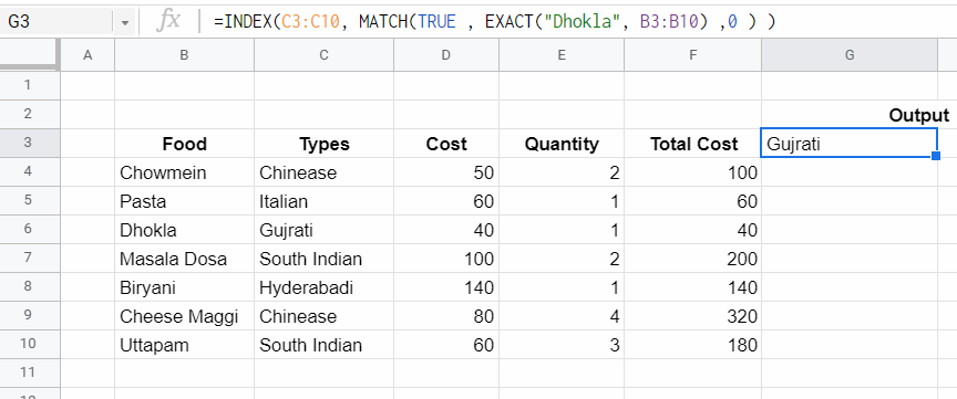
Example: Let say the task is to search for the Type Of Food “Dhokla” but in Case-Sensitive Way. This can be done using the formula-
=INDEX(C3:C10, MATCH(TRUE , EXACT("Dhokla", B3:B10) ,0))
Here the EXACT function will return True if the value in Column B3:B10 matches with “Dhokla” with the same case, else it will return False. Now MATCH function will apply in Column B3:B10 and search for a row with the Exact value TRUE. After that INDEX Function will retrieve the value of Column C3:C10 (Food Type Column) at the row returned by the MATCH function.
Multiple Criteria Lookup
One of the trickiest problems in Excel is a lookup based on multiple criteria. In other words, a lookup that matches on more than one column at the same time. In the example below, the INDEX and MATCH function and boolean logic are used to match on 3 columns-
- Food.
- Cost.
- Quantity.
To extract total cost.
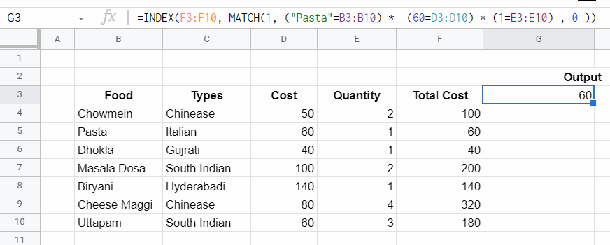
Example: Let’s say the task is to calculate the total cost of Pasta where
- Food: Pasta.
- Cost: 60.
- Quantity: 1.
So in this example, there are three criteria to perform a Match. Below are the steps for the search based on multiple criteria-
Step 1: First match Food Column (B3:B10) with Pasta using the formula:
"PASTA" = B3:B10
This will convert B3:B10 (Food Column) values as Boolean. That Is True where Food is Pasta else False.
Step 2: After that, match Cost criteria in the following manner:
60 = D3:D10
This will replace D3:D10 (Cost Column) values as Boolean. That is True where Cost=60 else False.
Step 3: Next step is to match the third criteria that are Quantity = 1 in the following manner:
1 = E3:E10
This will replace E3:E10 Column (Quantity Column) as True where Quantity = 1 else it will be False.
Step 4: Multiply the result of the first, second, and third criteria. This will be the intersection of all conditions and convert Boolean True / False as 1/0.
Step 5: Now the result will be a Column with 0 And 1. Here use the MATCH Function to find the row number of columns that contain 1. Because if a column is having the value 1, then it means it satisfies all three criteria.
Step 6: After getting the row number use the INDEX function to get the total cost of that row.
=INDEX(F3:F10, MATCH(1, ("Pasta"=B3:B10) * (60=D3:D10) * (1=E3:E10) , 0 ))
Here F3:F10 represents the Total Cost Column.
Excel is an incredibly powerful software – if you know how to leverage it. With so many functions and formula options, there’s something new to learn every day.

The INDEX/MATCH formula can help you find data points quickly without having to manually search for them and risk making mistakes.
![Download 10 Excel Templates for Marketers [Free Kit]](https://no-cache.hubspot.com/cta/default/53/9ff7a4fe-5293-496c-acca-566bc6e73f42.png)
Let’s dive into how that formula works and review some helpful use cases.
Understanding INDEX and MATCH Functions Individually
Before you can understand how to use the INDEX and match formula, it’s valuable to know how each function works on its own. That will offer some clarity on how both work together once combined.
The INDEX function returns a value or the reference to a value within a table or range based on the rows and columns you specify. Think of this function as a GPS – it helps you find data within a document but first, you need to narrow down the search area using rows and columns.
The MATCH function identifies a specific item in a range of cells then returns the relative position of that item in the range or the exact match.
For instance, say the range A1:A4 contains the values 15, 28, 49, 90. You want to know how the number «49» is relative to all values within the range. You would write the formula =MATCH(49,A1:A4,0) and it would return the number 3 because it’s the third number in the range. The 0 in the formula represents «exact match.»
Now that we’ve got the basics out of the way, let’s get into how to combine the formula and use it for multiple criteria.
The formula for the INDEX/MATCH formula is as follows: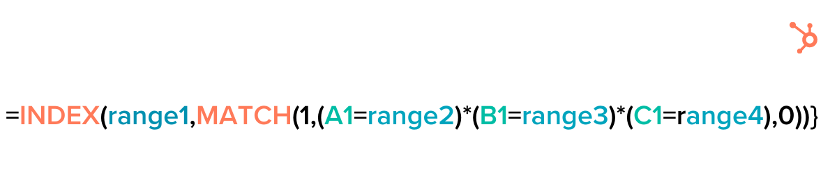
Here’s how each function works together: Match finds a value and gives you its location. It then feeds that information to the INDEX function, which turns that information into a result.
To see it in action, let’s use an example.
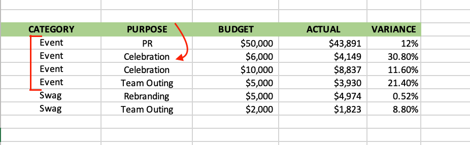
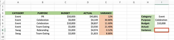
This Excel sheet features a marketing budget for two categories: Events and company swag gifts. There are four purposes: Public relations (PR), celebration, team outing, and rebranding. The sheet also includes the defined budget and the actual expense for each category.
This is where the INDEX and MATCH formula comes in handy when using it for multiple criteria. You can quickly find the answer(s) you’re looking for and limit mistakes that would happen when searching manually.
Say you want to know the variance for an event that had a purpose of celebration with a budget of 10,000 – here’s how you’d do it.
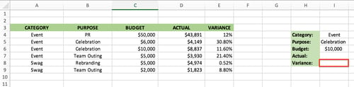
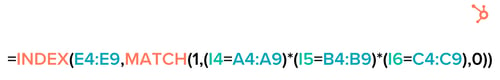
First, take note of the row numbers and columns. The answer you’re looking for will go in I8. Here’s how the formula will look:
Let’s break down how you get there.
1. Create a separate section to write out your criteria.
.jpg?width=600&name=excel%20index%20match%20with%20multiple%20criteria%20step%201%20(1).jpg) The first step in this process is by listing out your criteria and the figure you’re looking for somewhere in your sheet. You’ll need this section later to create your formula.
The first step in this process is by listing out your criteria and the figure you’re looking for somewhere in your sheet. You’ll need this section later to create your formula.
2. Start with the INDEX.
The formula starts with your GPS, which is the INDEX function. You’re looking for the variance, so you select rows E4 through E9, as that is where the answer will be.
3. Add your ranges.
The more columns you have, the more ranges you’ll need to add to narrow down your results.
As a reminder, you’re looking for the variance for an event that had a $10,000 budget and had a purpose of celebration. This means that you’ll have to tell Excel which rows hold the
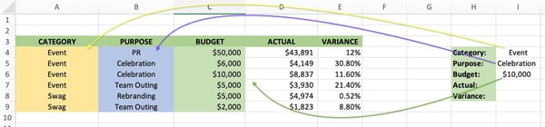
Starting with the «event,» criteria, you find it first in I4., with its range located in column A between rows 4 and 9.
Follow the same process for «celebration» – it’s in I5 and its range is B4 and B9. Lastly, the «$10,000» is in I6, with a range of C4 through C9.
The last step here is to add 0, which means you’re looking for an exact match.
That’s how you end up with this final formula:
4. Run the formula.
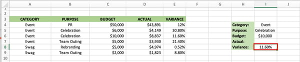
Because this is an array formula, you must press Ctrl+Shift+Enter to get the right results, unless you are using Excel 365.
There you have it!

If you’re using Excel and you’ve already learned how to use INDEX MATCH, you’re well on your way to becoming proficient with Excel lookups. What INDEX MATCH MATCH offers you is a more powerful version of the formula. Instead of just a vertical lookup, INDEX MATCH MATCH allows you to perform a matrix lookup, which is also known as a two-way lookup. This combination formula may initially seem complex because of its three individual formulas, but after you understand each component and how they interact, using this tool will become second nature to you. INDEX MATCH MATCH is one of several lookup formulas, which include OFFSET MATCH MATCH, VLOOKUP HLOOKUP and VLOOKUP MATCH, that you should learn to become adept in database theory.

Objective and When to Use
There’s really just one key condition that needs to be met before you can use INDEX MATCH MATCH:
A matrix lookup can only work if your data table has lookup values on both the top and left hand side.
Basically, your data needs to be in a matrix format. People usually create matrixes, with lookup values both vertically and horizontally, to cross reference two different fields. In the example below, we are cross referencing the field State with the field Year and showing the relevant data point for Sales.

Creating a matrix saves you space within your spreadsheet and is more visually appealing. However, most data sets are not organized in this fashion. In fact, if you follow proper database theory, your data actually should not have lookup values going both vertically and across your table. A properly formatted table would look like the example below:

Before moving forward, ensure that you are using the proper formula for your data set. There are several other lookup options you can choose from if your data does not fit the requirements for INDEX MATCH MATCH. For example, if you only have lookup values on the top of your data set, you should consider using HLOOKUP. If you only have lookup values on the very left hand column of your data set, you should consider using VLOOKUP or INDEX MATCH.
The Syntax
Below is the syntax for using this formula combination. Don’t worry if it doesn’t make sense now; the rest of this post will provide context for each component and we’ll review a more practical version of the syntax that’s easier to remember.
= INDEX ( array , MATCH ( lookup_value , lookup_array , 0 ) , MATCH ( lookup_value , lookup_array , 0 ) )
Not surprisingly, INDEX MATCH MATCH is based on the INDEX and MATCH formulas, which we will now go through in detail.
The INDEX Formula
The INDEX formula asks you to specify a reference within a range and returns a value. In its simplest form, you just indicate either a row or column as your range, specify a reference point, and the value that matches that reference point is returned. For example, if we were to select the left hand column of this table, and specify the reference “6”, the INDEX formula would return the value “WA”.
Now instead of using just selecting a single row or column, what you can also do with the INDEX formula is select an entire matrix, with multiple rows and columns, as your array. The key difference here is that, instead of just specifying a single appearance order as a reference, you must now provide both a vertical and horizontal reference to return your value. (Please note that the INDEX formula always takes the vertical reference first) Using the INDEX formula with a matrix reference represents the foundation of utilizing INDEX MATCH MATCH. The syntax for the INDEX formula by itself is as follows:
= INDEX ( array , row_number , column_number )
For example, let’s say we selected the entire sales data table, and then specified “6” as the row number and “4” as the column number. The INDEX formula performs the intuitive action of going down 6 rows and over 4 columns with the range we selected to return the value of “$261.04”.

The MATCH Formula
The MATCH formula asks you to specify a value within a range and returns a reference. The MATCH formula is basically the reverse of the INDEX formula. The two formulas have the exact same components, but the inputs and outputs are rearranged.
= MATCH ( lookup_value , lookup_array , 0 )
To give you an example of the MATCH formula, if we were to select the entire left hand column and then specify “WA” as our lookup value, the MATCH formula would return the number “6”. Please note that you have to put in a “0” as the last argument to ensure that the MATCH formula looks for an exact match.

How it Works
As mentioned before, when using the INDEX formula across a matrix it requires both a horizontal and vertical reference. The only additional complexity that INDEX MATCH MATCH adds is that the vertical and horizontal references are turned into MATCH formulas.
Putting it Together
Below is a simplified version of the syntax describing the inputs with the appropriate context for our goal. In case you get lost in the individual steps, you can always refer back to this notation.
= INDEX ( entire matrix , MATCH ( vertical lookup value, entire left hand lookup column , 0 ) , MATCH ( horizontal lookup value , entire top header row , 0 ) )
Step 1: Start writing your INDEX formula and select the entire table as your array

Step 2: When you get to the row number entry, input the MATCH formula and select your vertical lookup value for the lookup value input

Step 3: For the lookup array, select the entire left hand lookup column; please note that the height of this column selection should be exactly the same height as the array for the INDEX formula

Step 4: For the final argument in the MATCH formula, input 0 to perform an exact match and close out the MATCH formula

Step 5: Now that we’ve arrived at the column number entry of the INDEX formula, input another MATCH formula but this time select your horizontal lookup value for the lookup value input

Step 6: For this lookup array, select the entire top header row of the original grid you selected for the INDEX formula

Step 7: Repeating what we did for the previous MATCH formula, input “0” for an exact match and close both the MATCH formula and the INDEX formula with parentheses

What Excel Does
Excel must first calculate the result of the two MATCH formulas embedded within the INDEX formula. Since we know that “WA” is the sixth value down in the left hand column, and “2004” is the fourth value across in the top header row, those formulas become the values of 6 and 4 respectively. Once we’ve simplified those components, Excel essentially performs the exact same INDEX lookup that we demonstrated before; it goes down 6 rows and over 4 columns to pull the correct value of “$261.04”.
Summary
INDEX MATCH MATCH probably won’t be a formula you use often. Most of the time when dealing with databases and data tables, you’ll be using vertical lookups to query results. However, in situations where you absolutely do need to perform a matrix lookup, INDEX MATCH MATCH is the best option you have.
In this tutorial, we’ll dive into the powerful Excel INDEX and MATCH functions, which are essential for manipulating and analyzing large sets of data.
We’ll start by exploring what these functions do and how they retrieve specific information from a table, and then we’ll write INDEX and MATCH formulas together as an alternative to the VLOOKUP formula. We’ll also cover some practical use cases for INDEX and MATCH formulas.
Note: if you have Excel 2021 or later, or Microsoft 365 you should use the XLOOKUP function as this is easier and potentially more efficient.
Watch the INDEX and MATCH Video

Download the Excel File
Enter your email address below to download the sample workbook.
By submitting your email address you agree that we can email you our Excel newsletter.
How the INDEX function works:
The INDEX function returns the value at the intersection of a column and a row.
The syntax for the INDEX function is:
=INDEX(reference, row_num,[column_num], [area_num])
In English:
=INDEX( the range of your table, the row number of the table that your data is in, the column number of the table that your data is in, and if your reference specifies two or more ranges (areas) then specify which area*)
*Typically only one area is specified so the area_num argument can be omitted. The examples below don’t require area_num.
INDEX will return the value that is in the cell at the intersection of the row and column you specify.
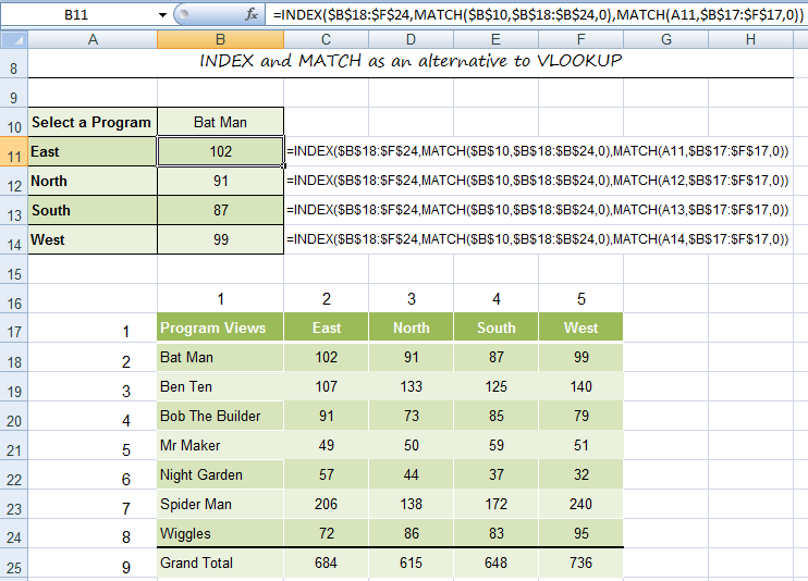
For example, looking at the table below in the range B17:F24 we can use INDEX to return the number of program views for Bat Man in the North region with a formula as follows:
=INDEX(B17:F24,2,3)
The result returned is 91.

On its own the INDEX function is pretty inflexible because you have to hard key the row and column number, and that’s why it works better with the MATCH function.
Note: You may have noticed that the INDEX function works in a similar way to the OFFSET function, in fact you can often interchange them and achieve the same results.
How the MATCH function works:
The MATCH function finds the position of a value in a list. The list can either be in a row or a column.
The syntax for the MATCH function is:
=MATCH(lookup_value, lookup_array, [match_type])
Now I don’t want to go all syntaxy (real word 🙂 ) on you, but I’d like to point out some important features of the [match_type] argument:
- The match_type argument specifies how Excel matches the lookup_value with values in lookup_array. You can choose from -1, 0 or 1 (1 is the default)
- [match_type] is an optional argument, hence the square brackets. If you leave it out Excel will use the default of 1, which means it will find the largest value that is <= to the lookup_value. The values in the lookup_array must be in ascending order when using 1 or omitting this argument..
- 0 will find the first value that is exactly equal to the lookup_value. The values in the lookup_array can be in any order.
- -1 finds the smallest value that is >= to the lookup_value. The values in the lookup_array must be in descending order, for example: TRUE, FALSE, Z-A, …2, 1, 0, -1, -2, …, and so on.
Ok, that’s enough of the syntax.
In English and using the previous example:
=MATCH(find what row Bat Man is on, in the column range B17:B24, match it exactly (for this we'll use 0 as our argument))
The result is row 2.
We can also use MATCH to find the column number like this:
=MATCH(find what column North is in, in the row range B17:F17, match it exactly (again we'll use 0 as our argument))
The result is column 3.
So in summary, the INDEX function returns the value in the cell you specify, and the MATCH function tells you the column or row number for the value you are looking up.
INDEX MATCH Together:
The INDEX and MATCH functions are a popular alternative to the VLOOKUP. Even though I still prefer VLOOKUP as it’s more straight forward to use, there are certain things the INDEX + MATCH functions can do that VLOOKUP can’t. More on that later.
Using the above example data we’ll use the INDEX and MATCH functions to find the program views for Bat Man in the East region.
=INDEX( the range of your table, replace this with a MATCH function to find the row number for Bat Man, replace this with a MATCH function to find the column number for East)
The formula will read like this:
=INDEX( return the value in the table range B17:F24 in the cell that is at the intersection of, MATCH( the row Bat Man is on) and, MATCH(the column East is in)
The formula looks like this:
=INDEX($B$18:$F$24,MATCH("Bat Man",$B$18:$B$24,0), MATCH(“East”,$B$17:$F$17,0))
So why would you put yourself through all that rigmarole when VLOOKUP can do the same job.
Reasons to use INDEX and MATCH rather than VLOOKUP
1) VLOOKUP can’t go left
Taking the table below, let’s say you wanted to find out what program was on the Krafty Kids channel.

VLOOKUP can’t do this because you’d be asking it to find Krafty Kids and then return the value in column B to the left, and VLOOKUP can only look to the right.
In comes INDEX and MATCH with a formula like this:
=INDEX($B$33:$B$40,MATCH("Krafty Kids",$C$33:$C$40,0))
And you get the answer; ‘Mr Maker’.
Notice only the Programs column (B) was referenced in INDEX’s array argument? This means we can omit INDEX’s column number argument as there’s only one column in the INDEX array.
2) Two way lookup
The table below has a drop down list in B1 that enables me to choose the Sales Person from the table, and a drop down list in A2 for the region. In B2 I’ve got an INDEX + MATCH formula that returns the sales that match my two criteria.
=INDEX(A4:J10,MATCH(A2,A4:A10,0),MATCH(B1,A4:J4,0))

Note: An alternative is to use a VLOOKUP and replace the hard keyed column number with a MATCH formula like this:
=VLOOKUP(A2,$A$4:$J$10,MATCH(B1,A4:J4,0),FALSE)
Ways to improve these formulas:
1) Use named ranges instead of $C$33:$C$40 etc. to make formulas more intuitive and quicker to create.
2) An alternative to using a named range is to convert the data to an Excel Table whereby Excel automatically gives the table a named range.
3) If there is nothing else in the columns other than your table you could use column references like this C:C which will search the whole column.