
Excel for Microsoft 365 Excel 2021 Excel 2019 Excel 2016 Excel 2013 Excel 2010 More…Less
Excel doesn’t have a default function that displays numbers as English words in a worksheet, but you can add this capability by pasting the following SpellNumber function code into a VBA (Visual Basic for Applications) module. This function lets you convert dollar and cent amounts to words with a formula, so 22.50 would read as Twenty-Two Dollars and Fifty Cents. This can be very useful if you’re using Excel as a template to print checks.
If you want to convert numeric values to text format without displaying them as words, use the TEXT function instead.
Note: Microsoft provides programming examples for illustration only, without warranty either expressed or implied. This includes, but is not limited to, the implied warranties of merchantability or fitness for a particular purpose. This article assumes that you are familiar with the VBA programming language, and with the tools that are used to create and to debug procedures. Microsoft support engineers can help explain the functionality of a particular procedure. However, they will not modify these examples to provide added functionality, or construct procedures to meet your specific requirements.
Create the SpellNumber function to convert numbers to words
-
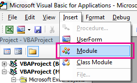
Use the keyboard shortcut, Alt + F11 to open the Visual Basic Editor (VBE).
-
Click the Insert tab, and click Module.

-
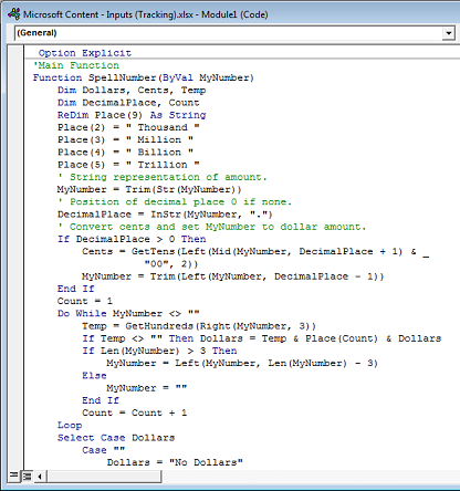
Copy the following lines of code.
Note: Known as a User Defined Function (UDF), this code automates the task of converting numbers to text throughout your worksheet.
Option Explicit 'Main Function Function SpellNumber(ByVal MyNumber) Dim Dollars, Cents, Temp Dim DecimalPlace, Count ReDim Place(9) As String Place(2) = " Thousand " Place(3) = " Million " Place(4) = " Billion " Place(5) = " Trillion " ' String representation of amount. MyNumber = Trim(Str(MyNumber)) ' Position of decimal place 0 if none. DecimalPlace = InStr(MyNumber, ".") ' Convert cents and set MyNumber to dollar amount. If DecimalPlace > 0 Then Cents = GetTens(Left(Mid(MyNumber, DecimalPlace + 1) & _ "00", 2)) MyNumber = Trim(Left(MyNumber, DecimalPlace - 1)) End If Count = 1 Do While MyNumber <> "" Temp = GetHundreds(Right(MyNumber, 3)) If Temp <> "" Then Dollars = Temp & Place(Count) & Dollars If Len(MyNumber) > 3 Then MyNumber = Left(MyNumber, Len(MyNumber) - 3) Else MyNumber = "" End If Count = Count + 1 Loop Select Case Dollars Case "" Dollars = "No Dollars" Case "One" Dollars = "One Dollar" Case Else Dollars = Dollars & " Dollars" End Select Select Case Cents Case "" Cents = " and No Cents" Case "One" Cents = " and One Cent" Case Else Cents = " and " & Cents & " Cents" End Select SpellNumber = Dollars & Cents End Function ' Converts a number from 100-999 into text Function GetHundreds(ByVal MyNumber) Dim Result As String If Val(MyNumber) = 0 Then Exit Function MyNumber = Right("000" & MyNumber, 3) ' Convert the hundreds place. If Mid(MyNumber, 1, 1) <> "0" Then Result = GetDigit(Mid(MyNumber, 1, 1)) & " Hundred " End If ' Convert the tens and ones place. If Mid(MyNumber, 2, 1) <> "0" Then Result = Result & GetTens(Mid(MyNumber, 2)) Else Result = Result & GetDigit(Mid(MyNumber, 3)) End If GetHundreds = Result End Function ' Converts a number from 10 to 99 into text. Function GetTens(TensText) Dim Result As String Result = "" ' Null out the temporary function value. If Val(Left(TensText, 1)) = 1 Then ' If value between 10-19... Select Case Val(TensText) Case 10: Result = "Ten" Case 11: Result = "Eleven" Case 12: Result = "Twelve" Case 13: Result = "Thirteen" Case 14: Result = "Fourteen" Case 15: Result = "Fifteen" Case 16: Result = "Sixteen" Case 17: Result = "Seventeen" Case 18: Result = "Eighteen" Case 19: Result = "Nineteen" Case Else End Select Else ' If value between 20-99... Select Case Val(Left(TensText, 1)) Case 2: Result = "Twenty " Case 3: Result = "Thirty " Case 4: Result = "Forty " Case 5: Result = "Fifty " Case 6: Result = "Sixty " Case 7: Result = "Seventy " Case 8: Result = "Eighty " Case 9: Result = "Ninety " Case Else End Select Result = Result & GetDigit _ (Right(TensText, 1)) ' Retrieve ones place. End If GetTens = Result End Function ' Converts a number from 1 to 9 into text. Function GetDigit(Digit) Select Case Val(Digit) Case 1: GetDigit = "One" Case 2: GetDigit = "Two" Case 3: GetDigit = "Three" Case 4: GetDigit = "Four" Case 5: GetDigit = "Five" Case 6: GetDigit = "Six" Case 7: GetDigit = "Seven" Case 8: GetDigit = "Eight" Case 9: GetDigit = "Nine" Case Else: GetDigit = "" End Select End Function -
Paste the lines of code into the Module1 (Code) box.
-
Press Alt + Q to return to Excel. The SpellNumber function is now ready to use.
Note: This function works only for the current workbook. To use this function in another workbook, you must repeat the steps to copy and paste the code in that workbook.
Top of Page
Use the SpellNumber function in individual cells
-
Type the formula =SpellNumber(A1) into the cell where you want to display a written number, where A1 is the cell containing the number you want to convert. You can also manually type the value like =SpellNumber(22.50).
-
Press Enter to confirm the formula.
Top of Page
Save your SpellNumber function workbook
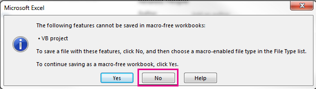
Excel cannot save a workbook with macro functions in the standard macro-free workbook format (.xlsx). If you click File > Save. A VB project dialog box opens. Click No.
You can save your file as an Excel Macro-Enabled Workbook (.xlsm) to keep your file in its current format.
-
Click File > Save As.
-
Click the Save as type drop-down menu, and select Excel Macro-Enabled Workbook.
-
Click Save.
Top of Page
See Also
TEXT function
Need more help?
Want more options?
Explore subscription benefits, browse training courses, learn how to secure your device, and more.
Communities help you ask and answer questions, give feedback, and hear from experts with rich knowledge.
Excel formulas let you automate your spreadsheets. But how do you use it in a Word document? Here are two ways to do it!
While you can always integrate Excel data into a Word document, it’s often unnecessary when all you need is a small table. It’s quite simple to create a table and use Excel formulas in a Word document. However, there is only a limited number of formulas that can be used.
For instance, if you’re trying to insert sales data in a table, you could add a column for sales, another one for total cost, and a third one for calculating profit using a formula. You can also calculate an average or a maximum for each of these columns.
Method 1: Paste Spreadsheet Data Into Word
If you already have data populated into a spreadsheet, you could just copy it into your Microsoft Word document.
- Copy the cells containing the data and open a Word document.
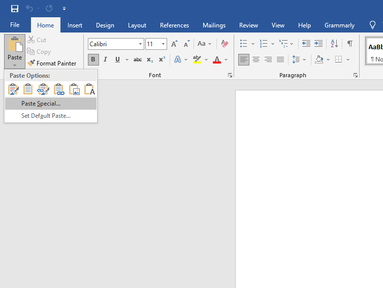
- From the top ribbon, click on the arrow under the Paste button, and click on Paste Special.

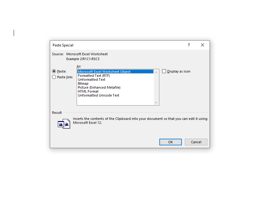
- You’ll see a new window pop-up where you’ll need to select what you want to paste the copied content as. Select Microsoft Excel Worksheet Object and select OK.

- Your data should now appear in the Word document, and the cells should contain the formulas as well.
If you want to make any edits, you can double-click on the pasted content, and your Word document will transform into an Excel document, and you’ll be able to do everything you would on a normal spreadsheet.
Method 2: Add Formulas in a Table Cell in Word
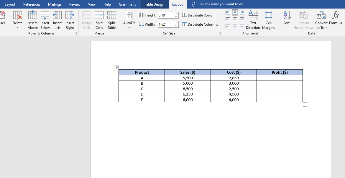
- Quickly insert a table in your Word document and populate the table with data.
- Navigate to the cell where you want to make your computations using a formula. Once you’ve selected the cell, switch to the Layout tab from the ribbon at the top and select Formula from the Data group.

Notice that there are two tabs called Layout. You need to select the one that appears under Table Tools in the ribbon.
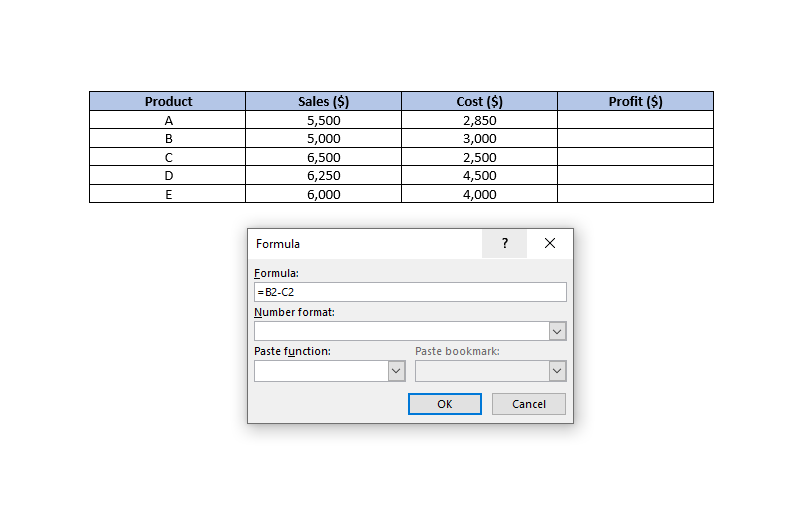
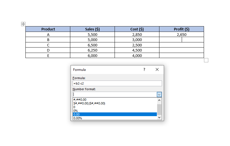
- When you click on Formula, you’ll see a small window pop up.
- The first field in the box is where you enter the formula you want to use. In addition to formulas, you can also perform basic arithmetic operations here. For instance, say you want to compute the profit, you could just use the formula:
=B2-C2Here, B2 represents the second cell in the second column, and C2 represents the second cell in the third column.

- The second field allows you to set the Number Format. For instance, if you wanted to calculate profit down to two decimal places, you could select a number format accordingly.

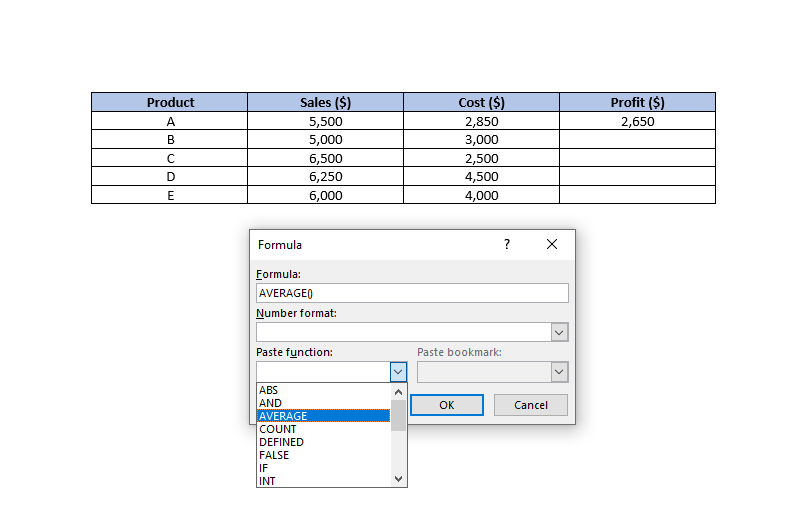
- The Paste Function field lists the formulas you can use in Word. If you can’t remember the name of a function, you could select one from the dropdown list, and it will automatically be added to the Formula field.

- When you’ve entered the function, click OK, and you’ll see the computed figure in the cell.
Positional Arguments
Positional arguments (ABOVE, BELOW, LEFT, RIGHT) can often make things simpler, especially if your table is relatively large. For instance, if you have 20 or more columns in your table, you could use the formula =SUM(ABOVE) instead of referencing each cell inside the parenthesis.
You can use positional arguments with the following functions:
- SUM
- AVERAGE
- MIN
- MAX
- COUNT
- PRODUCT
For instance, we could calculate the average sales for the above example using the formula:
=AVERAGE(ABOVE)
If your cell is at the center of the column, you can use a combination of positional arguments. For instance, you could sum up the values above and below a specific cell using the following formula:
=SUM(ABOVE,BELOW)
If you want to sum up the values from both the row and the column in a corner cell, you could use the following formula:
=SUM(LEFT,ABOVE)
Even though Microsoft Word offers only a few functions, they are quite robust in functionality and will easily help you create most tables without running into lack-of-functionality issues.
Updating Data and Results
Unlike Excel, Microsoft Word doesn’t update formula results in real-time. However, it does update the results once you close and re-open the document. If you want to keep things simple, just update the data, close, and re-open the document.
However, if you’d like to update the formula results as you continue to work on the document, you’ll need to select the results (not just the cell), right-click on them, and select Update Field.
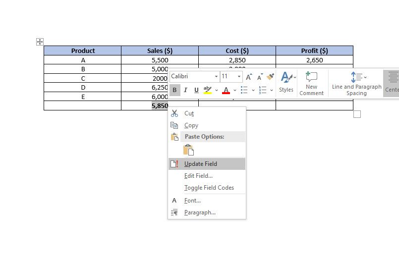
When you click Update Field, the formula’s result should update instantly.
Cell References
There are several ways to reference a cell in a Word document.
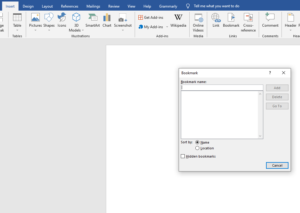
1. Bookmark Names
Let’s say you give your average sales value a bookmark name average_sales. If you don’t know how to give a cell a bookmark name, select the cell and navigate to Insert > Bookmark from the ribbon at the top.
Assume that the average sales value is a decimal value, and you’d like to convert it to an integer. You could reference the average sales value as ROUND(average_sales,0), and this will round the value down to its nearest integer.
2. RnCn References
The RnCn referencing convention allows you to reference a row, column, or a specific cell in a table. The Rn refers to the nth row, while the Cn refers to the nth column. If you wanted to refer to the fifth column and second row, for instance, you’d use R2C5.
You can even select a range of cells using the RnCn reference, much like you would in Excel. For instance, selecting R1C1:R1C6 selects the first six cells of the first row. For selecting the entire row in which you’re using the formula, just use R (or C for a column).
3. A1 References
This is the convention that Excel uses, and we’re all familiar with. The letter represents the columns, while the numbers represent the rows. For instance, A3 refers to the third cell in the first column.
Word Tables Made Easy
Hopefully, the next time you’ll need to use data on a Microsoft Word document, you’ll be able to do things much faster without having to first create a spreadsheet and then import it into your Word document.
Have you ever thought of an Excel formula that will convert Numbers to Words? i.e. A formula that can convert the number 456,571 into Four Hundred and Fifty Six Thousand Five Hundred and Seventy One.
In this blog post, I am sharing two Excel formulas that can convert Numbers in Words.
Pete M’s Formula
=CHOOSE(LEFT(TEXT(A1,"000000000"))+1,,"One","Two","Three","Four","Five","Six","Seven","Eight","Nine")&IF(--LEFT(TEXT(A1,"000000000"))=0,,IF(AND(--MID(TEXT(A1,"000000000"),2,1)=0,--MID(TEXT(A1,"000000000"),3,1)=0)," Hundred"," Hundred and "))&CHOOSE(MID(TEXT(A1,"000000000"),2,1)+1,,,"Twenty ","Thirty ","Forty ","Fifty ","Sixty ","Seventy ","Eighty ","Ninety ")&IF(--MID(TEXT(A1,"000000000"),2,1)<>1,CHOOSE(MID(TEXT(A1,"000000000"),3,1)+1,,"One","Two","Three","Four","Five","Six","Seven","Eight","Nine"),CHOOSE(MID(TEXT(A1,"000000000"),3,1)+1,"Ten","Eleven","Twelve","Thirteen","Fourteen","Fifteen","Sixteen","Seventeen","Eighteen","Nineteen"))&IF((--LEFT(TEXT(A1,"000000000"))+MID(TEXT(A1,"000000000"),2,1)+MID(TEXT(A1,"000000000"),3,1))=0,,IF(AND((--MID(TEXT(A1,"000000000"),4,1)+MID(TEXT(A1,"000000000"),5,1)+MID(TEXT(A1,"000000000"),6,1)+MID(TEXT(A1,"000000000"),7,1))=0,(--MID(TEXT(A1,"000000000"),8,1)+RIGHT(TEXT(A1,"000000000")))>0)," Million and "," Million "))&CHOOSE(MID(TEXT(A1,"000000000"),4,1)+1,,"One","Two","Three","Four","Five","Six","Seven","Eight","Nine")&IF(--MID(TEXT(A1,"000000000"),4,1)=0,,IF(AND(--MID(TEXT(A1,"000000000"),5,1)=0,--MID(TEXT(A1,"000000000"),6,1)=0)," Hundred "," Hundred and "))&CHOOSE(MID(TEXT(A1,"000000000"),5,1)+1,,,"Twenty ","Thirty ","Forty ","Fifty ","Sixty ","Seventy ","Eighty ","Ninety ")&IF(--MID(TEXT(A1,"000000000"),5,1)<>1,CHOOSE(MID(TEXT(A1,"000000000"),6,1)+1,,"One","Two","Three","Four","Five","Six","Seven","Eight","Nine"),CHOOSE(MID(TEXT(A1,"000000000"),6,1)+1,"Ten","Eleven","Twelve","Thirteen","Fourteen","Fifteen","Sixteen","Seventeen","Eighteen","Nineteen"))&IF((--MID(TEXT(A1,"000000000"),4,1)+MID(TEXT(A1,"000000000"),5,1)+MID(TEXT(A1,"000000000"),6,1))=0,,IF(OR((--MID(TEXT(A1,"000000000"),7,1)+MID(TEXT(A1,"000000000"),8,1)+RIGHT(TEXT(A1,"000000000")))=0,--MID(TEXT(A1,"000000000"),7,1)<>0)," Thousand "," Thousand and "))&CHOOSE(MID(TEXT(A1,"000000000"),7,1)+1,,"One","Two","Three","Four","Five","Six","Seven","Eight","Nine")&IF(--MID(TEXT(A1,"000000000"),7,1)=0,,IF(AND(--MID(TEXT(A1,"000000000"),8,1)=0,--RIGHT(TEXT(A1,"000000000"))=0)," Hundred "," Hundred and "))&CHOOSE(MID(TEXT(A1,"000000000"),8,1)+1,,,"Twenty ","Thirty ","Forty ","Fifty ","Sixty ","Seventy ","Eighty ","Ninety ")&IF(--MID(TEXT(A1,"000000000"),8,1)<>1,CHOOSE(RIGHT(TEXT(A1,"000000000"))+1,,"One","Two","Three","Four","Five","Six","Seven","Eight","Nine"),CHOOSE(RIGHT(TEXT(A1,"000000000"))+1,"Ten","Eleven","Twelve","Thirteen","Fourteen","Fifteen","Sixteen","Seventeen","Eighteen","Nineteen"))
This awesome formula was developed by Pete M, a commercial manager/consultant, and was shared with the public by the Excel MVP Leila Gharani in her blog post.
Note:
The formula assumes that you have the number in the cell A1.
The formula will ignore numbers after decimal.
Chandoo’s Formula
Here is a similar formula created by the Excel MVP Chandoo that will convert Numbers into English Words. This formula uses the LET function which is currently available to Office 365 subscribers.
=LET(
th, INT(A1/1000),
th.h, MOD(th/100, 10),
th.t, MOD(th, 100),
th.tens1, INT(th.t/10),
th.tens2, MOD(th.t,10),
h,MOD(A1/100,10),
t, MOD(A1,100),
tens1, INT(t/10),
tens2, MOD(t,10),
tys, {"twenty","thirty","fourty","fifty","sixty","seventy","eighty","ninety"},
upto19, {"one","two","three","four","five","six","seven","eight",
"nine","ten","eleven","twelve","thirteen","fourteen","fifteen",
"sixteen","seventeen","eighteen","nineteen"},
CONCAT(IF(th<1, "", IF(th.h>=1,INDEX(upto19,th.h)&" hundred ","") &
IF(th.t<1,"", IF(th.tens1<2,INDEX(upto19, th.t), INDEX(tys,th.tens1-1) & IF(th.tens2>=1,"-"&INDEX(upto19,th.tens2),"")))&
" thousand "),
IF(h>=1,INDEX(upto19,h)&" hundred ",""),
IF(t<1,"", IF(tens1<2,INDEX(upto19, t), INDEX(tys,tens1-1)& IF(tens2>=1,"-"&INDEX(upto19,tens2),"")))))
Chandoo, in his blog post has explained this formula in detail and has also done a video on the same.
Note:
This formula works up to numbers 999,999 only and will ignore numbers after decimal.
Download the workbook
Excel workbook with Formulas to convert Numbers into Words
UDF to convert Numbers into Words
If you are comfortable using VBA, the following is a blog post that explains a User Defined Function in Excel that will convert Numbers into Words.
User Defined Function to convert Numbers in Words

LET Function in Excel
New Dynamic Array Functions in Excel
Excel Tables
Formula Errors in Excel
STOCKHISTORY Function in Excel
Ever wanted to turn a number to words like 123,456 to One hundred twenty-three thousand four hundred fifty-six? You can use this elegant Excel formula to get convert number to words.

Excel Number to Words Formula
Below I have provided number to words Excel formula. It assumes you have input number in cell A1.
Note: This function can convert numbers up to 999,999 into words.
This works only in Office 365 with LET() function
If you have an older version of Excel, click here for VBA UDF.
The function:

=LET(
th, INT(A1/1000),
th.h, MOD(th/100, 10),
th.t, MOD(th, 100),
th.tens1, INT(th.t/10),
th.tens2, MOD(th.t,10),h,MOD(A1/100,10),
t, MOD(A1,100),
tens1, INT(t/10),
tens2, MOD(t,10),tys, {"twenty","thirty","fourty","fifty","sixty","seventy","eighty","ninety"},
upto19, {"one","two","three","four","five","six","seven","eight",
"nine","ten","eleven","twelve","thirteen","fourteen","fifteen",
"sixteen","seventeen","eighteen","nineteen"},CONCAT(IF(th<1, "",
IF(th.h>=1,INDEX(upto19,th.h)&" hundred ","") &
IF(th.t<1,"",
IF(th.tens1<2,INDEX(upto19, th.t), INDEX(tys,th.tens1-1) &
IF(th.tens2>=1,"-"&INDEX(upto19,th.tens2),"")))&
" thousand "),
IF(h>=1,INDEX(upto19,h)&" hundred ",""),
IF(t<1,"",
IF(tens1<2,INDEX(upto19, t), INDEX(tys,tens1-1)&
IF(tens2>=1,"-"&INDEX(upto19,tens2),"")))))
How this formula works?
In order to understand the number to words formula, you must first understand the newly introduced LET() function.
LET Excel Function:
LET function let’s us define variables to use with in the context of a formula. You can use LET function to shrink long formulas. Here is a quick example to explain the LET function.
Original formula:
=IF(SUM(A1:A10)>100, “Too high”,
IF(SUM(A1:A10)>20, “Medium”,
IF(SUM(A1:A10)>0, “Positive”,
“Could be zero or negative”)))
Same formula with LET():
=LET(s, SUM(A1:A10),
IF(s>100, “Too high”,
IF(s>20, “Medium”,
IF(s>0, “Positive”,
"Could be zero or negative”))))
We are using the SUM(A1:A10) several times in the original formula. In the LET() formula version, we start by defining a variable s that is equal to SUM(A1:A10) and then we use s in rest of the formula. This simplifies the formula and supposedly makes it faster too (as Excel would calculate SUM(A1:A10) once.
Learn more about LET function
LET function is introduced newly and available only in Excel 365. Click here to read the documentation on LET function.
Understanding Number to Words Excel formula
The process for turning number to words is not complicated. If you know how to convert words for numbers up to 999, then same logic is applied to thousands, millions and billions too.
So let’s understand the process for numbers up to 999.
- Define two arrays upto19 and tys to hold {one,two…,nineteen} and {twenty, thirty…,ninety} respectively.
- From the input number (say in A1), calculate these 4 numbers and store them in variables.
- h = MOD(A1/100,10)
- t = MOD(A1,100)
- tens1 = INT(t/10)
- tens2 = MOD(t,10)
- One way to look at these four variables is,
- h has hundreds digit
- t tells the last two digits
- tens1 tells the tens digit
- tens2 tells the ones digit
- So for an input number like 987, the 4 values would be h=9, t=87, tens1=8 and tens2=7
- Now, construct the words version of number by simply concatenating below:
- INDEX(upto19, h)
- ” hundred “
- if tens1<2 then INDEX(upto19, t)
- else INDEX(tys, tens1-1)&”-“&INDEX(upto19, tens2)
The actual formula needs a few more if conditions to stop the flow when you hit a round number (like 500 should five hundred with no other words after).
The process for numbers up to 999,999:
We just need to follow the same idea as above, but twice. Once for thousands and once for balance.
Known limitations of this formula:
- This formula works up to numbers 999,999 only. You can scale it up to work with numbers up to a billion easily, but the formula gets longer.
- It ignores any portion after decimal point. So 1003.20 becomes one thousand three.
- It doesn’t show “zero” for 0 input value. The output would be blank instead.
Excel Number to Words Formula — Video Explanation
Just in case your head hurts after all that explanation above, watch this video to understand how the formula works (plus a quick demo of LET function).
Excel Number to Words — VBA User Defined Formula
If you are not able to use the formula version then consider using below VBA UDF to convert number to words. This works up to a billion.
Public Function number2words(thisNum As Double) As String
    Dim bn As Integer, mn As Integer, th As Integer, h As Integer, retval As String

    On Error GoTo msg

    bn = Int(thisNum / 1000000000)
    mn = Int(thisNum / 1000000) Mod 1000
    th = Int(thisNum / 1000) Mod 1000
    h = thisNum Mod 1000

    If bn >= 1 Then
        retval = num2words999(bn) & " billion "
    End If
    If mn >= 1 Then
        retval = retval & num2words999(mn) & " million "
    End If
    If th >= 1 Then
        retval = retval & num2words999(th) & " thousand "
    End If
    retval = retval & num2words999(h)

    number2words = retval
    Exit Function

msg:
    number2words = "error"

End Function


Private Function num2words999(thisNum As Integer) As String
    'convert any number up to 999 to words

    Dim tys As Variant, upto19 As Variant

    tys = Array("twenty", "thirty", "fourty", "fifty", "sixty", "seventy", "eighty", "ninety")
    upto19 = Array("one", "two", "three", "four", "five", "six", "seven", "eight",
"nine", "ten", "eleven", "twelve", "thirteen", "fourteen", "fifteen",
"sixteen", "seventeen", "eighteen", "nineteen")

    Dim h As Integer, t As Integer, tens1 As Integer, tens2 As Integer, retval As String

    h = Int(thisNum / 100) Mod 10
    t = thisNum Mod 100
    tens1 = Int(t / 10)
    tens2 = t Mod 10

    If h >= 1 Then
        retval = upto19(h - 1) & " hundred "
    End If
    If t >= 1 Then
        If tens1 < 2 Then
            retval = retval & upto19(t - 1)
        Else
            retval = retval & tys(tens1 - 2)
            If tens2 >= 1 Then
                retval = retval & "-" & upto19(tens2 - 1)
            End If
        End If
    End If
    num2words999 = retval
End Function
How to use the Number2Words UDF?
You do not need prior VBA knowledge to use this function. It works like any other Excel function once you install it.
To install Number2Words function:
- You must have Personal Macros enabled. If not, click here to read on how to do that.
- Go to your Personal Macros workbook. Add a module or open an existing module.
- Paste the above code there.
How to use the Number2Words function:
To use this function on value in A1, simply write =Number2Words(A1)
Known limitations:
- This function ignores any portion after decimal point
- It doesn’t say “Zero” if input is 0 or blank. It would simply return blank.
- The results are not capitalized. Use Excel functions like PROPER() to do that.
- This function works up to 2 billion.
- If you email the result workbook to a colleague or client, then they cannot refresh the formula (unless they too have installed Number2Words UDF)
Download File — Number to Words Formula & UDF
Comments or suggestions please….
I hope you are finding the number to words formulas useful. Let me know if you are facing any issues or have suggestions for changing the outputs.
Indian version coming soon…
I am planning to add an Indian version of this (where instead of nine hundred eighty-seven thousand four hundred fifty-one the output would be nine lakhs eighty-seven thousand four hundred fity-one for example). I will update this page with such a formula (and UDF) once it is ready.
Share this tip with your colleagues

Get FREE Excel + Power BI Tips
Simple, fun and useful emails, once per week.
Learn & be awesome.
-
5 Comments -
Ask a question or say something… -
Tagged under
downloads, INDEX(), let function, new excel functions, udf, VBA, videos
-
Category:
Excel Howtos, VBA Macros

Welcome to Chandoo.org
Thank you so much for visiting. My aim is to make you awesome in Excel & Power BI. I do this by sharing videos, tips, examples and downloads on this website. There are more than 1,000 pages with all things Excel, Power BI, Dashboards & VBA here. Go ahead and spend few minutes to be AWESOME.
Read my story • FREE Excel tips book


Excel School made me great at work.
5/5

From simple to complex, there is a formula for every occasion. Check out the list now.

Calendars, invoices, trackers and much more. All free, fun and fantastic.

Power Query, Data model, DAX, Filters, Slicers, Conditional formats and beautiful charts. It’s all here.

Still on fence about Power BI? In this getting started guide, learn what is Power BI, how to get it and how to create your first report from scratch.

- Excel for beginners
- Advanced Excel Skills
- Excel Dashboards
- Complete guide to Pivot Tables
- Top 10 Excel Formulas
- Excel Shortcuts
- #Awesome Budget vs. Actual Chart
- 40+ VBA Examples
Related Tips
5 Responses to “Number to Words – Excel Formula”
-
 Nick Partridge says:
 As well as the Indian version, perhaps you could look into an English version as against the American version.
Things diverge after one hundred with one hundred one OR one hundred AND one.
I’m sure that it is always AND after n00 or n00,000 where there any of those zeros have a value. So five hundred thousand and sixteen. There could be two and’s seven hundred and eighty-six thousand four hundred and twenty-six. -
sandeep kothari says:
Chandoo, you are a genius.
-
-
That is a genius technique Robert. Thanks for posting it here.
-
-
David says:
100000000 One Hundred FALSE Million
Is there any reason for this error?
Leave a Reply
In my previous article, I had explained how to convert a number to words in Excel using VBA. I had written a number of code lines to achieve this. But I had never imagined that we can convert numbers to words by just using excel formulas. But one of our Excelforum users did it. I had never imagined that we could convert numbers into words.
This formula is used to convert a number into American currency. This formula can convert numbers from range cents to billions. The number can have two decimal places too.
This user with Id HaroonSid wrote a crazy formula. The formula is a page long and if I will mention it here now, it will cover the whole post. So, I have mentioned it at the end of the post. You can download the excel file below to check the formula.
The formula is too long to explain but I can explain the logic. This formula determines how long the number is. Then it uses the CHOOSE function to substitute numbers with the words. But this is not that easy. This formula Identifies once, tens, hundreds, thousands, millions and billions. It identifies which number comes in which section. Another complexity is this. The number 12 can be one or two in large numbers or Twelve. This adds up to a lot of complexity. But this man was able to solve this complexity and make this formula work efficiently.
So now I am mentioning the formula. This formula applies to B2. Any number written in B2 will be converted into words. This formula converts numbers into american currency dollars, but you can adjust it to convert into any currency or unit by just finding and replacing «Dollars» and «Cents». For example, if you want to convert numbers to Indian Rupee and Paise just find and replace.
So hold your chair. Here’s the formula.
So yeah, this is the formula. How do you like it? I hope it is useful to you. If you don’t want to use this, use the VBA method to convert numbers to words. If you have any doubts regarding this article or if you have any other Excel related questions, ask that too in the comments section below.
How to Convert Number to Words in Excel in Rupees : We can create a custom Excel formula to convert numbers to words in Indian rupees. I have created this custom function to convert numbers to words in terms of Indian rupees. You can download the macro file
13 Methods of How to Speed Up Excel | Excel is fast enough to calculate 6.6 million formulas in 1 second in Ideal conditions with normal configuration PC. But sometimes we observe excel files doing calculation slower than snails. There are many reasons behind this slower performance. If we can Identify them, we can make our formulas calculate faster.
Center Excel Sheet Horizontally and Vertically on Excel Page : Microsoft Excel allows you to align worksheet on a page, you can change margins, specify custom margins, or center the worksheet horizontally or vertically on the page. Page margins are the blank spaces between the worksheet data and the edges of the printed page
Split a Cell Diagonally in Microsoft Excel 2016 : To split cells diagonally we use the cell formatting and insert a diagonally dividing line into the cell. This separates the cells diagonally visually.
How do I Insert a Check Mark in Excel 2016 : To insert a checkmark in Excel Cell we use the symbols in Excel. Set the fonts to wingdings and use the formula Char(252) to get the symbol of a check mark.
How to disable Scroll Lock in Excel : Arrow keys in excel move your cell up, down, Left & Right. But this feature is only applicable when Scroll Lock in Excel is disabled. Scroll Lock in Excel is used to scroll up, down, left & right your worksheet not the cell. So this article will help you how to check scroll lock status and how to disable it?
What to do If Excel Break Links Not Working : When we work with several excel files and use formula to get the work done, we intentionally or unintentionally create links between different files. Normal formula links can be easily broken by using break links option.
How to use Excel VLOOKUP Function| This is one of the most used and popular functions of excel that is used to lookup value from different ranges and sheets.
How to use the Excel COUNTIF Function| Count values with conditions using this amazing function. You don’t need to filter your data to count specific value. Countif function is essential to prepare your dashboard.
Convert a number to words
To convert a number to words, the solution was always to create a very complex VBA macro. Some websites, like this one , give you an example of VBA code to do the job. But, if you aren’t familiar with VBA, it could be difficult to integrate this solution in your workbook.
Now with Excel 365 and the new LET function, you can convert a number to words. The formula is very complex and took a long time to develop. But despite this, there are certain points of the formula that must be analyzed before it can be used.
Characteristic of the formula
Before copying the complete formula and applying it to your workbook, it is important to analyze some points of the formula to avoid mistakes.
Principle of arrays in Excel
Excel 365 is the only version that can understand dynamic array (i.e. the result is returned in many cells).
An array is always written between brackets. But in function of the settings of your computer, there could be a difference for the separator.
For example, for a US setting,
- the separator for the rows is the semicolon (;)
- the separator for the columns is the comma (,)

Whatever your local settings, the row separator is always the semi-colon. But for the column separator, there is difference in function of your local settings.
- in France, the column separator is the period (.)
- in Spain, the separator in the backslash ().

Check this setting on your computer before to use this formula
Decimal separator
One of the trick of this formula is to detect the decimal numbers. Decimal number or not, the formula manage the 2 situations.
The trick lies in this part of the formula.
N, SUBSTITUTE(TEXT(A1, REPT(0,9)&».00″ ),».»,»0″)
Without going too deep in the detail of this formula, the decimal separator is mentioned 2 times in this part of the formula
- .00
- and the replacement symbol of the SUBSTITUTE function at the end «.»,»0″.
If you are working with the decimal comma (,), you must replace these 2 periods by commas in the function
N, SUBSTITUTE(TEXT(A1,REPT(0,9)&»,00″ ),»,»,»0″)
Dollars / Cents or nothing
The formula will always added Dollars after the units and Cents in case of decimals.
Denom, {«million», «thousand», «Dollars», «Cents»}
Now, if you do not wish to display the words Dollars and Cents, you simply have to remove these words BUT YOU MUST KEEP the empty quotes to respect the number of occurrences in the matrix.
Denom, {«million», «thousand», «»,»»}
Formula to convert a number to words
Here is the full formula. If it’s not working, change the parameters as it is explain before.
=LET(
Denom, {» Million, «;» Thousand «;» Dollars «;» Cents»},
Nums, {«»,»One»,»Two»,»Three»,»Four»,»Five»,»Six»,»Seven»,»Eight»,» Nine»},
Teens, {«Ten»,»Eleven»,»Twelve»,»Thirteen»,»Fourteen»,»Fifteen»,»Sixteen»,»Seventeen»,»Eighteen»,»Nineteen»},
Tens, {«»,»Ten»,»Twenty»,»Thirty»,»Forty»,»Fifty»,»Sixty»,»Seventy»,»Eighty»,»Ninety»},
grp, {0;1;2;3},
LET(
N, SUBSTITUTE( TEXT( A1, REPT(0,9)&».00″ ),».»,»0″),
H, VALUE( MID( N, 3*grp+1, 1) ), T, VALUE( MID( N, 3*grp+2, 1) ),
U, VALUE( MID( N, 3*grp+3, 1) ),
Htxt, IF( H, INDEX( Nums, H+1 ) & » Hundred «, «» ),
Ttxt, IF( T>1, INDEX( Tens, T+1 ) & IF( U>0, «-«, «» ), » » ),
Utxt, IF( (T+U), IF( T=1, INDEX( Teens, U+1 ), INDEX(Nums, U+1 ) ) ),
CONCAT( IF( H+T+U, Htxt & Ttxt & Utxt & Denom, «» ) )
)
)
This formula has been created by Peter Bartholomew 👏👍
Excel Functions : Convert Numbers into Words
Many times we need the amount in figures to be converted into words. This is a typical requirement for writing checks or any other financial reports. Microsoft Excel does not have standard function available for this requirement. However there are customised functions available on the Internet. One such solution is available at Allexperts.com.
Display Numbers to Text.
You need to copy this to your regular macro module. Once you have added it to your file you can use function SpellNumbers to convert any number into words easily as you use any other function of excel.
Function available at the net covers USD as currency, whereas I needed it in Indian Rupees. I have modified this to give results in any currency. The revised version gives me results as shown in the screen cast below.

Download excel file having this user defined function to convert numbers to words
Make sure that you enable macros to use this function. In case macros are disabled this function will not work in downloaded file
Syntex for the modified UDF is :-
SpellCurr(MyNumber, MyCurrency, MyCurrencyPlace, MyCurrencyDecimals, MyCurrencyDecimalsPlace)
where
MyNumber = Numeric Value you need to convert into words
MyCurrency = Name of your Currency — i.e. Dollar for USA
MyCurrencyPlace = Prefix or Suffix the currency, use «P» for Prefix and «S» for Suffix
MyCurrencyDecimals = Name of your Currency Decimals — i.e. Cent for USA
MyCurrencyDecimalsPlace = Prefix or Suffix the currency decimals, use «P» for Prefix and «S» for Suffix
Modified code given below for those who want to use it. Currency inputs are optional and you will not need to input currency details in case you are using it for Indian Currency. Still this can be used for any currency provided you give currency inputs.
You will need to copy this code to regular VBA module of your workbook
Function SpellCurr(ByVal MyNumber, _
Optional MyCurrency As String = "Rupee", _
Optional MyCurrencyPlace As String = "P", _
Optional MyCurrencyDecimals As String = "Paisa", _
Optional MyCurrencyDecimalsPlace As String = "S")'*****************************************************************************************************************
'* Based on SpellNumbers UDF by Microsoft, Which handles only Dollars as currency *
'* UDF modfied by Yogesh Gupta, smiley123z@gmail.com, Ygblogs.blogspot.com on July 21, 2009 *
'* UDF modified on September 04, 2009 to make currency inputs optional, by default it will use Indian Currency *
'* This modified UDF can be used for any currency in case you provide for currency inputs *
'* User can define the Prefix and Sufix place for Currency and CurrencyDecimals *
'* MyNumber = Numeric Value you need to convert into words *
'* MyCurrency = Name of your Currency - i.e. Dollar for USA *
'* MyCurrencyPlace = Prefix or Suffix the currency, use "P" for Prefix and "S" for Suffix *
'* MyCurrencyDecimals = Name of your Currency Decimals - i.e. Cent for USA *
'* MyCurrencyDecimalsPlace = Prefix or Suffix the currency decimals, use "P" for Prefix and "S" for Suffix *
'*****************************************************************************************************************Dim Rupees, Paisa, Temp
Dim DecimalPlace, CountReDim Place(9) As String
Place(2) = " Thousand "
Place(3) = " Million "
Place(4) = " Billion "
Place(5) = " Trillion "'String representation of amount.
MyNumber = Trim(Str(MyNumber))'Position of decimal place 0 if none.
DecimalPlace = InStr(MyNumber, ".")' Convert Paisa and set MyNumber to Rupee amount.
If DecimalPlace > 0 Then
Paisa = GetTens(Left(Mid(MyNumber, DecimalPlace + 1) & _
"00", 2))
MyNumber = Trim(Left(MyNumber, DecimalPlace - 1))
End IfCount = 1
Do While MyNumber <> ""
Temp = GetHundreds(Right(MyNumber, 3))
If Temp <> "" Then Rupees = Temp & Place(Count) & Rupees
If Len(MyNumber) > 3 Then
MyNumber = Left(MyNumber, Len(MyNumber) - 3)
Else
MyNumber = ""
End If
Count = Count + 1Loop
If MyCurrencyPlace = "P" Then
Select Case Rupees
Case ""
Rupees = MyCurrency & "s" & " Zero"
Case "One"
Rupees = MyCurrency & " One"
Case Else
Rupees = MyCurrency & "s " & Rupees
End Select
Else
Select Case Rupees
Case ""
Rupees = "Zero " & MyCurrency & "s"
Case "One"
Rupees = "One " & MyCurrency
Case Else
Rupees = Rupees & " " & MyCurrency & "s"
End Select
End IfIf MyCurrencyDecimalsPlace = "S" Then
Select Case Paisa
Case ""
Paisa = " Only"
Case "One"
Paisa = " and One " & MyCurrencyDecimals & " Only"
Case Else
Paisa = " and " & Paisa & " " & MyCurrencyDecimals & "s Only"
End Select
Else
Select Case Paisa
Case ""
Paisa = " Only"
Case "One"
Paisa = " and " & MyCurrencyDecimals & " One " & " Only"
Case Else
Paisa = " and " & MyCurrencyDecimals & "s " & Paisa & " Only"
End Select
End IfSpellCurr = Rupees & Paisa
End Function
'*******************************************
' Converts a number from 100-999 into text *
'*******************************************Function GetHundreds(ByVal MyNumber)
Dim Result As String
If Val(MyNumber) = 0 Then Exit Function
MyNumber = Right("000" & MyNumber, 3)
' Convert the hundreds place.
If Mid(MyNumber, 1, 1) <> "0" Then
Result = GetDigit(Mid(MyNumber, 1, 1)) & " Hundred "
End If' Convert the tens and ones place.
If Mid(MyNumber, 2, 1) <> "0" Then
Result = Result & GetTens(Mid(MyNumber, 2))
Else
Result = Result & GetDigit(Mid(MyNumber, 3))
End If
GetHundreds = Result
End Function'*********************************************
' Converts a number from 10 to 99 into text. *
'*********************************************
Function GetTens(TensText)Dim Result As String
Result = "" ' Null out the temporary function value.
If Val(Left(TensText, 1)) = 1 Then ' If value between 10-19...
Select Case Val(TensText)
Case 10: Result = "Ten"
Case 11: Result = "Eleven"
Case 12: Result = "Twelve"
Case 13: Result = "Thirteen"
Case 14: Result = "Fourteen"
Case 15: Result = "Fifteen"
Case 16: Result = "Sixteen"
Case 17: Result = "Seventeen"
Case 18: Result = "Eighteen"
Case 19: Result = "Nineteen"
Case Else
End Select
Else ' If value between 20-99...
Select Case Val(Left(TensText, 1))
Case 2: Result = "Twenty "
Case 3: Result = "Thirty "
Case 4: Result = "Forty "
Case 5: Result = "Fifty "
Case 6: Result = "Sixty "
Case 7: Result = "Seventy "
Case 8: Result = "Eighty "
Case 9: Result = "Ninety "
Case Else
End SelectResult = Result & GetDigit _
(Right(TensText, 1)) ' Retrieve ones place.
End If
GetTens = Result
End Function'*******************************************
' Converts a number from 1 to 9 into text. *
'*******************************************Function GetDigit(Digit)
Select Case Val(Digit)
Case 1: GetDigit = "One"
Case 2: GetDigit = "Two"
Case 3: GetDigit = "Three"
Case 4: GetDigit = "Four"
Case 5: GetDigit = "Five"
Case 6: GetDigit = "Six"
Case 7: GetDigit = "Seven"
Case 8: GetDigit = "Eight"
Case 9: GetDigit = "Nine"
Case Else: GetDigit = ""
End Select
End Function
Spell Currency Excel Addin avilable now
Numbers to Words , Convert Number to Words , Convert Number to Word , Number to Words , Number to Word , Number to Text , Number in Words , Number to Letters , Convert Number to Text , VBA Number to Text , Number to Text Function , Numeric to Text
I found this formula below to convert amounts to words for google spreadsheets and it works perfectly. But now I want to use it in excel 2010 and I get a lot of errors. I also cannot use VBA. Thanks for any help.
=if(or(isBlank(A1),not(isNumber(A1)),A1>=power(10,15)),ifError(1/0,»Error»),trim(arrayFormula(concatenate(if(trunc(mod(A1,power(10,{15,12,9,6,3}))/power(10,{12,9,6,3,0}))<100,»»,choose(int(trunc(mod(A1,power(10,{15,12,9,6,3}))/power(10,{12,9,6,3,0}))/100),» One»,» Two»,» Three»,» Four»,» Five»,» Six»,» Seven»,» Eight»,» Nine») & » Hundred») & if(mod(trunc(mod(A1,power(10,{15,12,9,6,3}))/power(10,{12,9,6,3,0})),100)<>0,if(trunc(mod(A1,power(10,{15,12,9,6,3}))/power(10,{12,9,6,3,0}))>100,» And»,if(A1>power(10,{15,12,9,6,3}),choose({1,2,3,4,5},»»,»»,»»,»»,» And»),»»)),»») & if(mod(trunc(mod(A1,power(10,{15,12,9,6,3}))/power(10,{12,9,6,3,0})),100)=0,»»,if(mod(trunc(mod(A1,power(10,{15,12,9,6,3}))/power(10,{12,9,6,3,0})),100)<20,choose(mod(trunc(mod(A1,power(10,{15,12,9,6,3}))/power(10,{12,9,6,3,0})),100),» One»,» Two»,» Three»,» Four»,» Five»,» Six»,» Seven»,» Eight»,» Nine»,» Ten»,» Eleven»,» Twelve»,» Thirteen»,» Fourteen»,» Fifteen»,» Sixteen»,» Seventeen»,» Eighteen»,» Nineteen»),choose(int(mod(trunc(mod(A1,power(10,{15,12,9,6,3}))/power(10,{12,9,6,3,0})),100)/10),»»,» Twenty»,» Thirty»,» Forty»,» Fifty»,» Sixty»,» Seventy»,» Eighty»,» Ninety») & if(mod(mod(trunc(mod(A1,power(10,{15,12,9,6,3}))/power(10,{12,9,6,3,0})),100),10)=0,»»,»-» & choose(mod(mod(trunc(mod(A1,power(10,{15,12,9,6,3}))/power(10,{12,9,6,3,0})),100),10),»One»,»Two»,»Three»,»Four»,»Five»,»Six»,»Seven»,»Eight»,»Nine»)))) & if(trunc(mod(A1,power(10,{15,12,9,6,3}))/power(10,{12,9,6,3,0}))=0,»»,choose({1,2,3,4,5},» Trillion»,» Billion»,» Million»,» Thousand»,»»)))) & if(A1>=2,» Rand»,if(A1>=1,» Rand»,»»)) & if((round(A1-trunc(A1),2)*100=0)+(A1<1),»»,» And») & if(round(A1-trunc(A1),2)*100=0,»»,if(round(A1-trunc(A1),2)*100=1,» One Cent»,if(round(A1-trunc(A1),2)*100<20,choose(round(A1-trunc(A1),2)*100,» One»,» Two»,» Three»,» Four»,» Five»,» Six»,» Seven»,» Eight»,» Nine»,» Ten»,» Eleven»,» Twelve»,» Thirteen»,» Fourteen»,» Fifteen»,» Sixteen»,» Seventeen»,» Eighteen»,» Nineteen»),choose(int(round(A1-trunc(A1),2)*100/10),»»,» Twenty»,» Thirty»,» Forty»,» Fifty»,» Sixty»,» Seventy»,» Eighty»,» Ninety») & if(mod(round(A1-trunc(A1),2)*100,10)=0,»»,»-» & choose(mod(round(A1-trunc(A1),2)*100,10),»One»,»Two»,»Three»,»Four»,»Five»,»Six»,»Seven»,»Eight»,»Nine»))) & » Cent»))))