
Содержание
- Tips for improving Excel’s performance
- Performance tips for specific circumstances
- Links to popular topics
- Get the latest updates, and let us know what you think
- Excel performance: Performance and limit improvements
- SUMIFS, AVERAGEIFS, COUNTIFS, MAXIFS, MINIFS Improvements
- RealTimeData Function (RTD)
- VLOOKUP, HLOOKUP, MATCH improvements
- LAA memory improvement for 32-bit Excel
- Full column references
- Structured references
- Filtering, sorting, and copy/pasting
- Copying conditional formats
- Adding and deleting worksheets
- New functions
- Other updates to Excel 2016 for Windows
- Excel 2010 performance improvements
- Large data sets and the 64-bit version of Excel
- Shapes
- Calculation improvements
- Multi-core processing
- PowerPivot
- HPC Services for Excel 2010
- Conclusion
- See also
- Support and feedback
Tips for improving Excel’s performance
Here on the Excel team, we’re always working to improve Excel’s performance and stability. We constantly seek customer feedback regarding what we can do to make a better product, and implement positive suggestions whenever we can. In fact, many of the improvements we have made recently were direct responses to customer pain points. For instance, we discovered that many heavy, institutional Excel users were less than thrilled with Excel’s performance when they upgraded from Office 2010 to newer versions.
We listened, and the team set to addressing those areas where we could make the most significant performance improvements possible and deliver them in the shortest time. For example:
We’ve again made substantial performance improvements to Aggregation functions (SUMIFS, COUNTIFS, AVERAGEIFS, etc.), RealtimeData (RTD), and lots more for significant decreases in calculation time.
We’ve made substantial performance improvements to the VLOOKUP, HLOOKUP and MATCH functions, which also resulted in significant decreases in calculation time — and for Microsoft 365 customers, XLOOKUP and XMATCH offer better flexibility and even more performance improvements.
We improved Excel’s memory allocation with Large Address Aware Excel, increased copy/paste speed, undo, conditional formatting, cell editing and selection, scrolling, filtering, file open, and programmability.
We’ve re-engineered Excel’s calculation engine with the release of dynamic array functions, which replace Excel’s legacy Ctrl+Shift+Enter (CSE) array functions. These functions add capabilities to Excel that were difficult to achieve in earlier versions of Excel. For instance, you can now sort and filter a list with formulas instead of doing it manually.
To continue on the performance theme, this article lists multiple tips for improving Excel’s performance.
Performance tips for specific circumstances
General slowness when editing in the grid or when switching worksheets
Slowness when moving an Excel window or when using ALT+ shortcut keys after upgrading to Windows 10
General slowness on a machine with no dedicated graphics processor or with an old graphics card or driver
Slowness when editing one cell after another
Slowness when using multiple high-resolution monitors with per-monitor dynamic high definition aware Office functionality
Parts of Excel turn white or gray when you run VBA code
Unresponsiveness or high CPU on Windows 10 when many Excel windows are open and Background Application Manager runs a periodic background scan
Slowness pressing ALT+ shortcut keys in Excel
Slowness when Excel launches
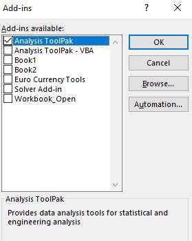
Open Excel in Safe Mode to see if the slowness is caused by add-ins
You see out-of-memory issues opening multiple workbooks
Power Query is taking too long to load to a query to a worksheet.
Power Query is taking too long to add a query to Preview Data in the Power Query Editor.
Name: DisableWindowHinting
Type: REG_DWORD
Value: 1
Name: UseAsyncRibbonKeytips
Type: REG_DWORD
Value: 1
Links to popular topics
Read about the Excel team’s latest performance improvements.
Excel can now use more of your system memory than ever before, even with 32-bit Office.
Read about methods for being smarter with formulas and how they calculate.
This is a broad recap of some of our latest improvements.
Tips and tricks for optimizing your VBA code from the Excel team.
If you create macros or Office add-ins, you’ll want to review this article.
More tips on how to improve Excel’s calculation performance, including with User Defined Functions (UDFs) for VBA.
In Excel 2013 and later versions, each Excel window can contain only one workbook, and each has its own ribbon. This is called Single Document Interface (SDI). By default when you open a new workbook, it will be displayed in another Excel window, even though it is the same Excel instance.
Get the latest updates, and let us know what you think
If you want to get the latest updates for Excel, then you can join the Office Insiders program.
Give us feedback by pressing the Smiley button in the upper right-hand corner of the Excel pane. Make sure to put the term «ExcelPERF» somewhere in your comments, so we can keep an eye out for it.
Ask a question in the Excel Tech Community. This is a vibrant community of Excel enthusiasts who are waiting to answer your questions. We also passively monitor the forums to keep an eye on any emerging trends or issues.
If you have a feature you’d like to request, please send us your feedback to help us prioritize new features in future updates. See How do I give feedback on Microsoft Office for more information.
Источник
Excel performance: Performance and limit improvements
Applies to: Excel | Excel M365| Excel 2016 | Excel 2013 | Excel 2010 | Office 2016 | SharePoint Server 2010 | VBA
Excel M365 introduces new features that you can use to improve performance when you are working with large or complex Excel workbooks
SUMIFS, AVERAGEIFS, COUNTIFS, MAXIFS, MINIFS Improvements
In Office 365 version 2005 monthly channel and later, Excel’s SUMIFS, AVERAGEIFS, COUNTIFS, MAXIFS, and MINIFS as well as their singular counterparts SUMIF, AVERAGEIF, and COUNTIF are much faster than Excel 2010 aggregating string data in the spreadsheet. These functions now create an internal cached index for the range being searched in each expression. This cached index is reused in any subsequent aggregations that are pulling from the same range.
The effect is dramatic: For example calculating 1200 SUMIFS, AVERAGEIFS, and COUNTIFS formulas aggregating data from 1 million cells on a 4 core 2 GHz CPU that took 20 seconds to calculate using Excel 2010, now takes 8 seconds only, on Excel M365 2006.
RealTimeData Function (RTD)
In Excel M365 version 2002 monthly channel or later, Excel’s RealTimeData (RTD) function is much faster than Excel 2010 calculating data in the spreadsheet. We removed bottlenecks in its underlying memory and data structures as well as made it thread-safe to allow it to be calculated on all available threads of Multithreaded recalculation (MTR).
For example simulating 125,000 RTD updates for stock topics like «Last Price», «Ask», «Bid» to calculate values like «Trade Volume», «Market Value», «Trade Gain/Loss» etc. in 500,0000 cells in all, took 47 seconds using Excel 2010 and only 7 seconds using Excel M365 Version 2002, on the same hardware.
Another positive effect of making RTD function thread-safe, is that Multithreaded recalculation (MTR) doesn’t need to be paused to run RTD function anymore. This improves performance noticeably when running RTD along with lots of other calculations.
For example, we ran a workbook with 10,000 RTD and 10,000 VLOOKUP functions, with each VLOOKUP depending on an RTD function result. Without thread-safe RTD full recalcuation took 10.20 seconds and with thread-safe RTD it took 5.84 seconds.
VLOOKUP, HLOOKUP, MATCH improvements
In Office 365 version 1809 and later, Excel’s VLOOKUP, HLOOKUP, and MATCH for exact match on unsorted data is much faster than ever before when looking up multiple columns (or rows with HLOOKUP) from the same table range.
These lookup functions now create an internal cached index for the column range being searched. This cached index is reused in any subsequent lookups that are pulling from the same row (VLOOKUP and MATCH) or column (HLOOKUP). The effect is dramatic: lookups on 5 different columns in the same table range can be up to 4 times faster than the same lookups using Excel 2010 or Excel 2016, and the improvement is larger as more columns are looked up.
For example calculating 100 rows of these 5 VLOOKUP formulas took 37 seconds to calculate using Excel 2010 and only 12 seconds using Excel 2016.
LAA memory improvement for 32-bit Excel
Although the 64-bit version of Excel has large virtual memory limits, the 32-bit version has only 2 GBs of virtual memory. Some customers use the 32-bit version because some third-party add-ins and controls are not available in the 64-bit version.
The 32-bit versions of Excel 2013 and Excel 2016 now have Large Address Aware (LAA) enabled. This will minimize out-of-memory error messages.
LAA doubles available virtual memory from 2 GB to 4 GB on 64-bit versions of Windows, and increases available virtual memory from 2 GB to 3 GB on 32-bit versions of Windows.
To download a tool that shows how much virtual memory is available and how much is being used, see Excel Memory Checking Tool.
Full column references
In earlier versions of Excel, workbooks using large numbers of full column references and multiple worksheets (for example =COUNTIF(Sheet2!A:A,Sheet3!A1) ) might use large amounts of memory and CPU when opened or when rows were deleted.
Excel 2016 Build 16.0.8212.1000 reduces the memory and CPU used in these circumstances.
In a sample test on a workbook with 6 million formulas, using full column references failed with an out-of-memory message at 4 GB of virtual memory with Excel 2013 LAA and with Excel 2010, but only used 2 GB of virtual memory with Excel 2016.
Structured references
In Excel 2013 and earlier versions, editing tables where formulas in the workbook use structured references to the table was slow. This led to the perception that tables should not be used with large numbers of rows. This issue no longer occurs in Excel 2016.
For example, an editing operation that took 1.9 seconds in Excel 2013 and Excel 2010 took about 2 milliseconds in Excel 2016.
Filtering, sorting, and copy/pasting
We’ve made a number of improvements to the response time when filtering, sorting, and copy/pasting in large workbooks.
In Excel 2013, after filtering, sorting, or copy/pasting many rows, Excel could be slow responding or would hang. Performance was dependent on the count of all rows between the top visible row and the bottom visible row. These operations are much faster after we improved the internal calculation of vertical user interface positions in Build 16.0.8431.2058.
Opening a workbook with many filtered or hidden rows, merged cells, or outlines could cause high CPU load. We introduced a fix in this area in Build 16.0.8229.1000.
After pasting a copied column of cells from a table with filtered rows where the filter resulted in a large number of separate blocks of rows, the response time was very slow. This has been improved in Build 16.0.8327.1000.
A sample test on copy/pasting 22,000 rows filtered from 44,000 rows showed a dramatic improvement:
- For a table, the time went from 39 seconds in Excel 2013 and 18 seconds in Excel 2010 to 2 seconds in Excel 2016.
- For a range, the time went from 30 seconds in Excel 2013 and 13 seconds in Excel 2010 to instantaneous in Excel 2016.
Copying conditional formats
In Excel 2013, copy/pasting cells containing conditional formats could be slow. This has been significantly improved in Excel 2016 Build 16.0.8229.0.
A sample test on copying 44,000 cells with a total of 386,000 conditional format rules showed a substantial improvement:
- Excel 2010: 70 seconds
- Excel 2013: 68 seconds
- Excel 2016: 7 seconds
Adding and deleting worksheets
When adding and deleting large numbers of worksheets, a sample test on Excel 2016 Build 16.0.8431.2058 shows a 15%–20% improvement in speed compared to Excel 2013, but 5-10% slower than Excel 2010.
New functions
Excel 2016 Build 16.0.7920.1000 introduces several useful worksheet functions:
- MAXIFS and MINIFS extend the COUNTIFS/SUMIFS family of functions. These functions have good performance characteristics. Use them to replace equivalent array formulas.
- TEXTJOIN and CONCAT let you easily combine text strings from ranges of cells. Use them to replace equivalent VBA UDFs.
Other updates to Excel 2016 for Windows
For more details about the month-by-month improvements to Excel 2016, see What’s new in Excel 2016 for Windows.
Excel 2010 performance improvements
Based on user feedback about Excel 2007, Excel 2010 introduces improvements to several features.
| Feature | Improvement |
|---|---|
| Printer and page layout view | To improve performance of basic user interactions in page layout view, such as entering data, working with formulas or setting margins, Excel 2010 caches the printer settings and introduces optimized rendering calculations. Caching the printer settings reduces the number of network calls and reduces the dependency on a slow or unresponsive printer. In addition, connecting to the printer is cancelable so that the user does not have to wait for a slow or unresponsive printer. |
| Charts | Starting in Excel 2010, the rendering speed of charts has increased, especially with large data sets, and text-rendering performance has improved. In addition, Excel 2010 caches an image of a chart and uses the cached version when possible, to avoid unnecessary calculations and rendering. |
| VBA solutions | Improvements to the object model and the way it interacts with Excel increases the performance speed of many VBA solutions when run in Excel 2010 compared with Excel 2007. |
Large data sets and the 64-bit version of Excel
The 64-bit version of Excel 2010 is not constrained to 2 GB of RAM like the 32-bit version applications nor upto 4 GB of RAM like the Large Address Aware 32-bit version applications. Therefore, the 64-bit version of Excel 2010 enables users to create much larger workbooks. The 64-bit version of Windows enables a larger addressable memory capacity, and Excel is designed to take advantage of that capacity. For example, users are able to fill more of the grid with data than was possible in previous versions of Excel. As more RAM is added to the computer, Excel uses that additional memory, allows larger and larger workbooks, and scales with the amount of RAM available.
In addition, because the 64-bit version of Excel enables larger data sets, both the 32-bit and 64-bit versions of Excel 2010 introduce improvements to common large data set tasks such as entering and filling down data, sorting, filtering, and copying and pasting data. Memory usage is also optimized to be more efficient in both the 32-bit and 64-bit versions of Excel.
For more information about the 64-bit version of Office 2010, see Compatibility Between the 32-bit and 64-bit Versions of Office 2010 and for choosing between 64-bit and 32-bit, see Choose between the 64-bit or 32-bit version of Office.
Shapes
Excel 2010 introduces significant improvements in the performance of graphics in Excel. At a high level, these improvements are in two areas: scalability and rendering.
The scalability improvements have a large impact in Excel scenarios because of the large number of graphics contained on worksheets. Often, this large number of shapes is created accidentally by copying and pasting data from a website, or by commonly run automation that creates shapes, but never removes them. This large number of graphics, combined with the way that graphics relate to the data grid in Excel, presents several unique performance challenges. Improvements in Excel 2010 increase the performance speed for worksheets that contain many shapes.
In addition, starting in Excel 2010, support for hardware acceleration improves rendering. Excel 2010 also introduces performance improvements to the Select method of the Shape object in the VBA object model.
| Feature | Improvement |
|---|---|
| Basic use | The first set of improvements made in Excel 2010 surrounds basic use scenarios. These scenarios include operations and features such as sorting, filtering, inserting or resizing rows or columns, or merging cells. When these operations occur, it may be necessary to update the position of a graphic object on the grid. In the worst-case scenario, it is necessary to make an update to every single object on the worksheet. In Excel 2010, performance of these basic scenarios improves even when there are thousands of objects on the worksheet. These improvements were not achieved with a single feature or fix, but through a dedicated focus on performance that included improving the shape lookup mechanism, testing stress files, and investigating obstructions. |
| Text links | A text link on a shape is created when the user specifies a formula, for example «=A1», that defines the text for a given shape. These particular shapes were prone to cause performance issues on sheets with a large number of objects and/or when changes were made to cell content. Starting in Excel 2010, the way Excel tracks and updates these shapes has improved to optimize performance for changing cell content. This work improves scenarios such as typing a new value in a cell or performing complex object model operations. |
| Big Grid | Starting in Excel 2007, the size of the grid expanded from 65,000 rows to over one million rows. This increase caused some performance and rendering issues when working with graphics objects in the new regions of the larger grid. Starting in Excel 2010, Excel optimizes functionality that relies on using the top left of the grid as the origin to improve the experience of working with graphics in the new regions of the grid. Rendering fidelity and performance are improved relative to Excel 2007. |
| Rendering: Hardware acceleration | Starting in Excel 2010, improvements were made to the graphics platform by adding support for hardware acceleration when rendering 3-D objects. While the GPU can render these objects faster than the CPU, the experience in Excel 2010 depends on the content on your worksheet. If you have a sheet full of 3-D shapes, you’ll see more benefit from the hardware acceleration improvements than on a worksheet with only 2-D shapes (which don’t leverage the GPU). |
Calculation improvements
Starting in Excel 2007, multithreaded calculation improved calculation performance.
Starting in Excel 2010, additional performance improvements were made to further increase calculation speed. Excel 2010 can call user-defined functions asynchronously. Calling functions asynchronously improves performance by allowing several calculations to run at the same time. When you run user-defined functions on a compute cluster, calling functions asynchronously enables several computers to be used to complete the calculations. For more information, see Asynchronous User-Defined Functions.
Multi-core processing
Excel 2010 made additional investments to take advantage of multi-core processors and increase performance for routine tasks. Starting in Excel 2010, the following features use multi-core processors: saving a file, opening a file, refreshing a PivotTable (for external data sources, except OLAP and SharePoint), sorting a cell table, sorting a PivotTable, and auto-sizing a column.
For operations that involve reading and loading or writing data, such as opening a file, saving a file, or refreshing data, splitting the operation into two processes increases performance speed. The first process gets the data, and the second process loads the data into the appropriate structure in memory or writes the data to a file. In this way, as soon as the first process begins reading a portion of data, the second process can immediately start loading or writing that data, while the first process continues to read the next portion of data. Previously, the first process had to finish reading all the data in a certain section before the second process could load that section of the data into memory or write the data to a file.
PowerPivot
PowerPivot refers to a collection of applications and services that provide an end-to-end approach for creating data-driven, user-managed business intelligence solutions in Excel workbooks. PowerPivot for Excel is a data analysis tool that delivers unmatched computational power directly within Excel. Leveraging familiar Excel features, users can transform large quantities of data from almost any source with amazing speed into meaningful information to get the answers they need in seconds.
PowerPivot also integrates with SharePoint. In a SharePoint farm, PowerPivot for SharePoint is the set of server-side applications, services, and features that support team collaboration on business intelligence data. SharePoint provides the platform for collaborating and sharing business intelligence across the team and larger organization. Workbook authors and owners publish and manage the business intelligence that they develop to their SharePoint sites.
For more information about PowerPivot, see PowerPivot Overview.
HPC Services for Excel 2010
With a wealth of statistical analysis functions, support for constructing complex analyses, and broad extensibility, Excel 2010 is the tool of choice for analyzing business data. As models grow larger and workbooks become more complex, the value of the information generated increases. However, more complex workbooks also require more time to calculate. For complex analyses, it is common for users to spend hours, days, or even weeks completing such complex workbooks.
One solution is to use Windows HPC Server 2008 to scale out Excel calculations across multiple nodes in a Windows high-performance computing (HPC) cluster in parallel. There are three methods for running Excel 2010 calculations in a Windows HPC Server 2008 based cluster: running Excel workbooks in a cluster, running Excel user-defined functions (UDFs) in a cluster, and using Excel as a cluster service-oriented architecture (SOA) client.
For more information about HPC Services for Excel 2010, see Accelerating Excel 2010 with Windows HPC Server 2008 R2.
Conclusion
Excel 2016 introduces performance and limitation improvements focused on increasing Excel’s ability to efficiently handle large and complex workbooks. These improvements allow Excel to scale along with hardware, improving performance as the CPU and RAM capacity of computers expand.
See also
Support and feedback
Have questions or feedback about Office VBA or this documentation? Please see Office VBA support and feedback for guidance about the ways you can receive support and provide feedback.
Источник
There are various advice about how to speed up Excel. Also we’ve published an article about how to increase the performance of Excel (actually it’s our most read article). But we’ve asked ourselves: Which of these advice really help? Furthermore: How much time can you save with it? That’s why we measured how long Excel calculates under different conditions.
We found some surprising results.
The method for measuring the Excel performance
Our goal is not to get some laboratory results. We rather want to know, how Excel behaves under realistic work conditions.
Before we jump right in with the results we must take a quick look at the method. Please scroll down to the end of this article for the method and hardware in detail.
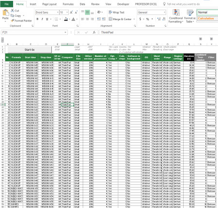
- Measuring is done with an Excel file with 100,000 VLOOKUP formulas.
- A VBA Macro determines the exact calculation time.
- Only one variable is changed at a time.
- The tests are done on two computers: A new Lenovo ThinkPad and a late 2013 (“medium-good”) MacBook Pro (the detailed specification are at the end).
- Each setting is calculated 6 times. The first run is removed as well as the slowest and fastest run.
- If the results are not as expected or the impact is especially large, the specific test was repeated under different settings.
Results of the Excel performance
64 bit Excel vs. 32 bit Excel
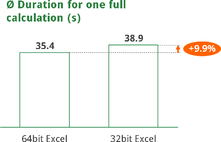
The first question: Is the 64bit version of Excel really faster than the 32bit version?
The results are quite clear: The 32bit version of Excel is app. 10% slower than the 64bit version of Excel. Or the other way around: The 64bit version is 9% faster than 32bit.
As of now, Microsoft still recommends going with the 32bit version. But the arguments supporting 32bit are mainly that some (older) add-ins and data connections might not support 64bit. So maybe you should just try it and see, if the 64bit version works for you.
Optimized computer vs. not optimized computer
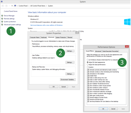
Windows provides the functionality to optimize the computer for best performance.
Therefore, go to settings, system and advanced system settings as shown on the image no. 1 to 3.
We tested one time with all tick marks set (“Optimized for best appearance”). Then we compared it to the option “Adjust for best performance” (no ticks set).
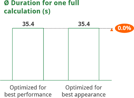
In our test we couldn’t verify that optimizing the computer for best performance really speeds up Excel. As there doesn’t seem to be a difference in calculation time we recommend you to stay with your preferred layout option.
Region Germany vs. Region USA
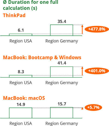
We actually didn’t plan this test but rather found out by coincidence. The regional settings seem to have a big impact on the performance of Excel.
The German numeric system uses commas as decimal character and points as thousands separator. Therefore Excel formulas don’t use commas for separating arguments but rather semicolon. A VLOOKUP in Excel with German regional settings looks like this:
=VLOOKUP(A2;B:C;2;FALSE)
We compared the region “German (Germany)” with “English (USA)”. Surprisingly, these settings seem to have a major impact on the calculation performance of Excel.
As the difference is so huge (+400 – +500% of calculation duration), we repeated this test under the three environments of the ThinkPad, Windows on a MacBook under Bootcamp as well as Excel for macOS.
More surprisingly, the difference seems to come up only under Windows.
A possible explanation could be that Excel first translates the formulas into “English” before really calculating them.

Such big difference of calculation times led us to investigate further: How are the calculation times with other region settings. We compared the top languages around the world and found even more interesting results.
The table on the right hand side shows the reduction of calculation time if you switch from a region to “English (USA)”.
Hindi, Punjabi and Arabic even reduce the time needed for calculating by even -97%. Choosing “English (USA)” instead of Spanish, French, German, Russian or Portuguese reduces the calculation time by around 80%. Only Japanese and China are almost as fast as English.
Number of processors
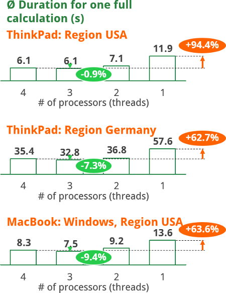
We assumed the following relation: The more processors you use, the faster Excel calculates.
Excel provides the option to choose the number of processors to calculate on. As our test computer has 4 processors, we could choose between 1 to 4 processors.
First of all, the relation of number of processors and performance turns out to be true. It seems like the difference in calculation time is between 63% and 94% higher with 4 processors than just one (highlighted in orange) .
But there is one surprise: Calculating on 3 processors (it says 3 threads on 4 processors) seems to be slightly faster than on 4 processors (highlighted in green). Unfortunately, we don’t have an explanation for this behavior. Therefore if you have an idea of why 3 threads are slightly faster, please let us know.
Large file vs. small file
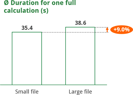
We always wondered, if the file size has an impact on the calcution time. That’s why we prepared a test file with many more worksheets, just containing hard values (no additional formulas). The “large” file had 25 more worksheets and had the file size 26,116 KB whereas the “small” test file was just 2,336 KB.
There seems to be a significant difference in performance: Calculating the same number of formulas in a large file seems to be significantly slower than in a small Excel file. So the conclusion: You can save up to 8% of time by removing old data from your file (the actual number of course depends on the amount of data you have in your file).
Close all other programs?
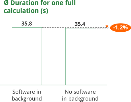
We often hear the suggestion to close all other programs in order to speed up Excel. But do other programs really have an impact?
We let our test file calculation once without any other (obvious) software in the background and tried to simulate some “normal” working environment with the following programs open:
- Microsoft Outlook
- Microsoft PowerPoint
- Spotify
- WhatsApp Desktop
- Microsoft OneNote
- Chrome
We didn’t use these programs but just let them stay opened in the background.
Our test revealed that closing all other programs in the background reduces the calculation time by app. 1.2%. Of course, this highly depends on your hardware and the CPU and RAM usage of the other programs.
2 steps in 2 formulas vs. 2 steps in 1 formula
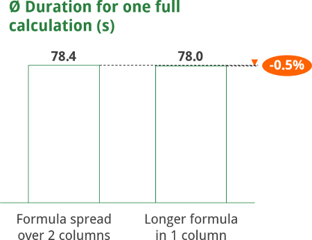
Is it better to have an additional column or to put two formulas into one Excel column?
In order to answer this question we’ve set up a VLOOKUP within a VLOOKUP. So basically the result of the first VLOOUP is the search value for the second VLOOKUP. We compare two options:
- Each lookup formula in 1 column so that the first column with the first VLOOKUP is the input value for the second column. The formula is divided into two columns.
- Having a longer formula within 1 column.
The direct comparison shows: Having a longer formula in 1 column is slightly faster. You can save app. 0,5% of calculation time.
Do you want to boost your productivity in Excel?
Get the Professor Excel ribbon!

Add more than 120 great features to Excel!
Which lookup formula is the fastest?
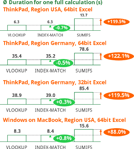
There are basically 3 different formulas for conducting a simple lookup:
- VLOOKUP
- INDEX/MATCH
- SUMIFS
We’ve already evaluated in detail which formula to use in which case. The only aspect we haven’t really talked about is the performance.
The difference between VLOOKUP and SUMIFS as well as INDEX-MATCH and SUMIFS seems to be very clear: The calculation time of SUMIFS is app. 90% to 120% longer than either VLOOKUP or INDEX-MATCH (highlighted in orange color). If we put it the other way: VLOOKUP reduces the calculation time by 53% towards a SUMIFS.
The difference between VLOOKUP and INDEX-MATCH seems just minor and it seems under different condition, INDEX-MATCH is in some cases faster and in other cases VLOOKUP shows a better performance (highlighted in green color). That’s also the reason why we repeated this test 4 times under different conditions.
SUMIFS vs. SUMIF
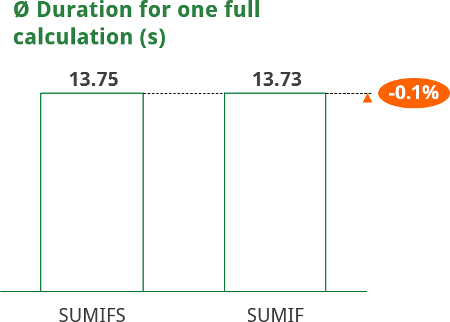
Is there a difference between the “old” SUMIF and the “newer” SUMIFS?
In order to compare these two formulas, we only used SUMIFS with one criteria. So both formulas have 3 arguments each.
The results: SUMIF seem insignificantly faster. You could save around 0.1% of time by using SUMIF instead of SUMIFS. That’s why we recommend only using SUMIFS. It has more advantages towards SUMIF as the structure is clearer and – of course – you can use up to 127 criteria.
MAX() vs. IF
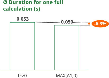
This is quite a specific case: The two following formulas get the same result:
- =IF(A1>0,A1,0)
- =MAX(A1,0)
But which one of them is faster in terms of calculation speed?
In our test, the second option (MAX) is app. 6.3% faster. So if you use this IF function a lot, you might want to replace it with the MAX formula. But please keep in mind that 100,000 rounds of calculation just take 0.05s. So unless you aren’t having a workbook full with this formula you won’t save much time in absolut numbers.
Windows 10 vs. macOS
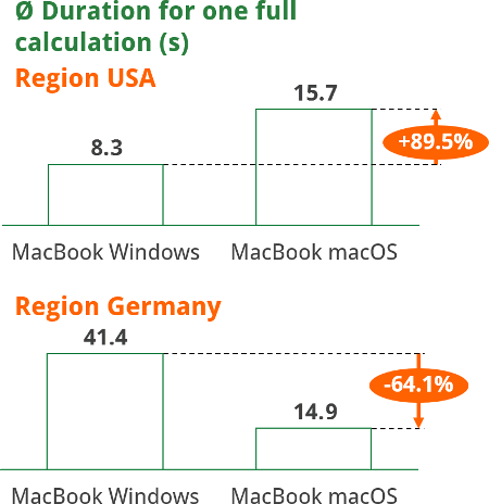
Honestly, we are not sure how much you can compare those two systems in terms of Excel calculation time. In order to at least get an indication of the performance, we used a MacBook having both macOS Sierra and Windows 10 (Anniversary edition). Windows runs under Bootcamp. Both systems have their latest versions of Excel.
Our test shows once again: the regional settings are more important than the operating system. With the region English (USA) macOS is much slower (needs almost 90% more time).
If you set the region to Germany, macOS is significantly faster.
In conclusion: If you choose the region USA you should use Windows under Bootcamp for your Excel calculation. If you choose Germany, stay under macOS.
Sheet order
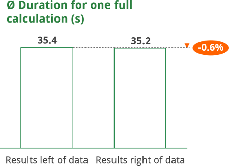
Especially with old versions of Excel it was recommended to choose the sequence of worksheets carefully. Excel was supposed to calculate faster if the formula sequence was aligned with the worksheet order: The formulas on the second worksheet should depend on the first worksheet. Consequently the formulas on the third worksheet should depend on the second and so on.
So is this rule of thumb still up to date?
Our test shows that if the worksheet with the formulas (or results) is located on the right side of the input data, you can save 0.6% of time.
Faster computer: 2013 MacBook vs. 2016 ThinkPad
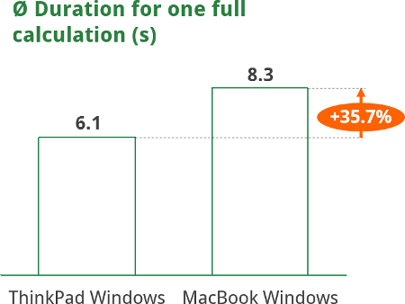
This test only has limited validity. But it’s still interesting to see how an older MacBook (late 2013) compares to a new ThinkPad (2016).
As assumed, the ThinkPad is faster. The MacBook with Windows under Bootcamp needs 36% more time for calculating. Or the other way around: The ThinkPad needs 26% less time than the MacBook.
One interesting side observation: As a result of the different cooling systems of the two computers, the fan of the ThinkPad was running the whole time on high power. Opposite on the MacBook: the fan didn’t turn on during the whole test.
Summary
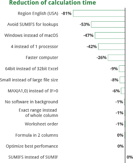
We measured which tips actually increase the performance of Excel.
- The biggest impact on the calculation time is easily achieved: Switch your computer to the region “English (USA)” (if not done yet).
- Avoiding the SUMIFS formula for lookup also cuts the calculation time by half. Of course only if you use it a lot.
- If you have the choice: Use Windows instead of macOS for your calculation.
- This one is possible for most users: Make sure you calculate on all available processors (or in our case also 3 threads lead to a slightly faster performance).
- Surprisingly, a faster computer (in our case MacBook Pro late 2013 vs. 2016 ThinkPad) “only” decreases the calculation time by 26%.
- If you can, switch to 64bit Excel instead of the default 32bit version.
- Also, now it might be time to remove all old data from your Excel file.
- Just a minor effect, but still -6% of calculation time: Use =MAX(A1,0) instead of =IF(A1>0,A1,0.
- All other advice only have a minor impact. For example closing all other programs, using the exact cell ranges, changing the worksheet order or optimizing the computer for best performance.
More information about the method, hardware and software
The method and environment in detail
The measuring is done with a simple VBA macro. Simplified speaking, it writes down a start time stamp, initiates a full recalculation and also notes the time when done. In order to eliminate outliers and getting more stable results, we eliminated all data with the following criteria:
- Each specification runs 6 times.
- The first result will be removed.
- Of the remaining 5 runs the slowest and fastest were also eliminated.
- Of the remaining 3 runs, an average time is calculated.
- All add-ins were disabled.
In order to be able to compare the results, a base setting was defined. For each simulation, one variable was changed. The base case:
- ThinkPad.
- Excel, 64bit.
- German regional settings.
- Small file without additional data.
- Base formula: 100,000 x VLOOKUP.
- The test file contains three worksheets (in this order):
- The VLOOKUP formula on Sheet1.
- The data for the VLOOKUP on Sheet2.
- The results (time stamps) on Sheet3.
Download the test file
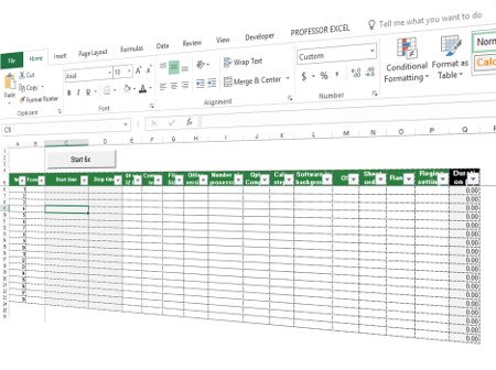
Please feel free to download the test file and do your own analysis. Just press start and Excel will do 6 full calculations. We already prepared some columns but you can of course modify them. Only column C and D must stay the same as the start and end time will be written here.
- File name: Test_File_Performance.xlsm
- File size: 2.4 MB
Notebook specifications
We used these versions of Excel: Excel 2016 64bit, Excel 2016 32bit and Excel Mac 2016.
Notebook 1: Lenovo ThinkPad
- Processor: Intel® Core™ i7-6500U CPU 2.50 GHz
- RAM: 8.00 GB
- Operating System: Windows 10 Pro, “Anniversary Edition”
Notebook 2: MacBook Pro, Late 2013
- Processor: Intel® Core™ i5, 2.4 GHz
- RAM: 8.00 GB
- Operating System: macOS Sierra (10.12.1) and Windows 10 Pro, “Anniversary Edition” with Bootcamp
If there is one thing that unites us all, it has to be the frustration to keep up with a slow excel spreadsheets.
While the impact on the performance may be negligible when there is less data, it becomes more profound as you add more and more data/calculations to the workbook.
9 out of 10 times, an Excel user would complain about the slow Excel spreadsheets. And there is hardly anything you can do about it.
Well, that’s NOT completely true.
The way Excel has been made, it does get slow with large data sets. However, there are many speed-up tricks you can use to improve the performance of a slow Excel spreadsheet.
10 Tips to Handle Slow Excel Spreadsheets
Here are 10 tips to give your slow Excel spreadsheet a little speed boost, and save you some time and frustration (click to jump to that specific section).
- Avoid Volatile Functions (you must).
- Use Helper Columns.
- Avoid Array Formulas (if you can).
- Use Conditional Formatting with Caution.
- Use Excel Tables and Named Ranges.
- Convert Unused Formulas to Values.
- Keep All Referenced Data in One Sheet.
- Avoid Using Entire Row/Column in References.
- Use Manual Calculation Mode.
- Use Faster Formula Techniques.
1. Avoid Volatile Formulas
Volatile formulas are called so because of a reason. Functions such as NOW, TODAY, INDIRECT, RAND, OFFSET etc. recalculate every time there is a change in the workbook.
For example, if you use NOW function in a cell, every time there is a change in the worksheet, the formula would be recalculated and the cell value would update.
This takes additional processing speed and you end up with a slow excel workbook.
As a rule of thumb, avoid volatile formulas. And if you can’t, try and minimize its use.
2. Use Helper Columns
Helper columns are one of the most under-rated design constructs in Excel. I have seen many people shy away from creating helper columns.
DON’T DO That.
The biggest benefit of using ‘Helper Columns’ is that it may help you avoid array formulas.
Now don’t get me wrong. I am not against array formulas. Rather I believe these could be awesome in some situations. But it when you try to do it all with one long formula, it does impact the performance of your Excel workbook. A couple of array formulas here and there shouldn’t hurt, but in case you need to use it in many places, consider using helper columns.
Here are some Examples where helper columns are used:
- Automatically Sort Data in Alphabetical Order using Formula.
- Dynamic Excel Filter – Extract Data as you Type.
- Creating Multiple Drop-down Lists in Excel without Repetition.
3. Avoid Array Formulas
Array formulas have its own merits – but speed is not one of those.
As explained above, array formulas can take up a lot of data (cell references), analyze it, and give you the result. But doing that takes time.
If there is a way to avoid array formulas (such as using helper column), always take that road.
4. Use Conditional Formatting with Caution
I absolutely love conditional formatting. It makes bland data look so beautiful. Instead of doing the comparison yourself, now you can simply look at a cell’s color or icon and you’d know how it compares with others.
But.. here is the problem.
Not many Excel users know that Excel Conditional Formatting is volatile.
While you may not notice the difference with small data sets, it can result in a slow excel spreadsheet if applied on large data sets, or applied multiple times.
Word of advice – Use it Cautiously.
Also read: How to Remove Conditional Formatting in Excel (Shortcut + VBA)
5. Use Excel Tables and Named Ranges
Excel Table and Named Ranges are two amazing features that hold your data and makes referencing super easy. It may take a while to get used to it, but when you start using it, life becomes easy and fast.
In creating data-driven dashboards, it is almost always a good idea to convert your data into an Excel Table.
It also has an added advantage of making your formulas more comprehensible.
For example, what’s easier to understand?
=Sales Price-Cost Price OR =SUM(A1:A10)-SUM(G1:G10)
6. Convert Unused Formulas to Static Values
This is a no-brainer. When you don’t need it, don’t keep it.
Lots of formulas would result in a slow Excel workbook. And if you have formulas that are not even being used – you know who to blame. As a rule of thumb, if you don’t need formulas, it’s better to convert them into a static value (by pasting as values).
Read More: How to quickly convert formulas to values.
7. Keep All Referenced Data in One Sheet
This may not always be possible, but if you can do this, I guarantee your Excel sheet would become faster.
The logic is simple – formulas in your worksheet don’t have to go far to get the data when it is right next to it in the same sheet.
8. Avoid Using the Entire Row/Column as Reference (A:A)
The only reason I have this one on the list is that I see a lot of people using the entire row/column reference in formulas. This is a bad practice and should be avoided.
While you may think that the row/column only has a few cells with data, Excel doesn’t think that way. When you reference an entire row/column, Excel acts it as a good servant and check it anyways. That takes more time for calculations.
9. Use Manual Calculation Mode
I am just repeating what million people have already said in various forums and blogs. Using Manual calculation gives you the flexibility to tell excel when to calculate, rather than Excel taking its own decisions. This is not something that speeds up your Excel workbook, but if you have a slow Excel spreadsheet, it definitely saves time by not making Excel recalculate again and again.
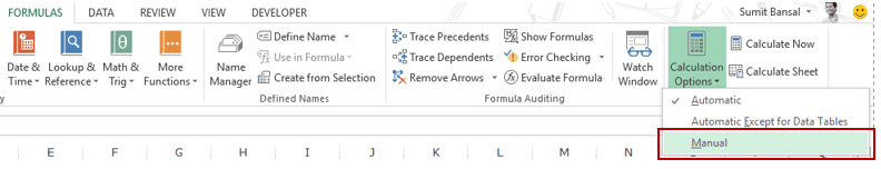
- To switch to manual mode, go to Formula Tab –> Calculation Options –> Manual (press F9 key to recalculate)
10. Use Faster Formulas Techniques
Excel gives you a lot of formulas and formula-combos to do the same thing. It is best to identify and use the fastest ones.
Here are a couple of examples:
- Use IFERROR instead of IF and ISERROR combo (unless you are using Excel 2003 or earlier, which does not have IFERROR).
- Use MAX(A1,0) instead do IF(A1>0,A1,0) – This is a cool tip that I learned from Mr. Excel aka Bill Jelen. His research shows that MAX option is 40% faster than IF option (and I am ready to take this stat on his face value).
- Use the INDEX/MATCH combo, instead of VLOOKUP – This may raise a lot of eyebrows, but the truth is, there is no way VLOOKUP can be faster if you have 100’s of columns of data. The world is moving towards INDEX/MATCH, and you should make the shift too.
[If you are still confused about what to use, here is a head-on-head comparison of VLOOKUP Vs. INDEX/MATCH]. - Use — (double negatives) to convert TRUE’s and FALSE’s to 1’s and 0’s (instead of multiplying it by 1 or adding 0 to it). The speed improvement is noticeable in large data sets.
Is this an exhaustive list? Absolutely NOT. These are some good ones that I think are worth sharing as a starting point. If you are looking to master Excel-Speed-Up techniques, there is some good work done by a lot of Excel experts.
Here are some sources you may find useful:
- 75 Speed-up tips by Chandoo (smartly done by crowdsourcing).
- Decision Models Website.
- Mr. Excel Message Board (explore this and you would find tons of tips).
I am sure you also have many tips that can help tackle slow excel spreadsheets. Do share it with us here in the comment section.
I also have one request. The pain of working with a slow excel spreadsheet is something many of us experience on a daily basis. If you find these techniques useful. share it with others. Ease their pain, and earn some goodness 🙂
You May Also Like the Following Excel Links:
- 24 Excel Tricks to Make You Sail through Day-to-day work.
- 10 Super Neat Ways to Clean Data in Excel Spreadsheets.
- 10 Excel Data Entry Tips You Can’t Afford to Miss.
- Creating and Using a drop-down List in Excel.
- Reduce Excel File Size.
- How to Recover Unsaved Excel Files.
- Free Online Excel Training (7-part video course)
- Arrow Keys not Working in Excel | Moving Pages Instead of Cells

Excel is fast enough to calculate 6.6 million formulas in 1 second in Ideal conditions with normal configuration PC. But sometimes we observe excel files doing calculation slower than snails. There are many reasons behind this slower performance. If we can Identify them, we can make our formulas calculate faster. In this article, we will learn how can we make our excel files calculate faster.
These are the methods that can make your excel calculate faster.
1 : Reduce the complexity and number of formulas
I know I said that excel can calculate 6.6 million formulas in one second. But in Ideal conditions. Your computer is not only using Excel program right. It has other tasks running.
Excel does not only have formulas. It has data, tables, charts, add inns, etc. All these increase the burden on the processor. And when you have thousands of complex formulas running, it slows down the processor.
So, if it is possible, reduce the number of the formulas and complexity of formulas.
2. Use all the processors available for Excel.
Some times your computer is busy in processing other threads. Making all the processors available for excel will increase the speed of Excel significantly. To do so follow these steps:
Go to file —> Options —> Advanced. Here scroll down and find Formulas Section. Select the «Use all the processors in this computer: 4». This will allow excel to use all the processors available on the system. It will make the calculations fast.
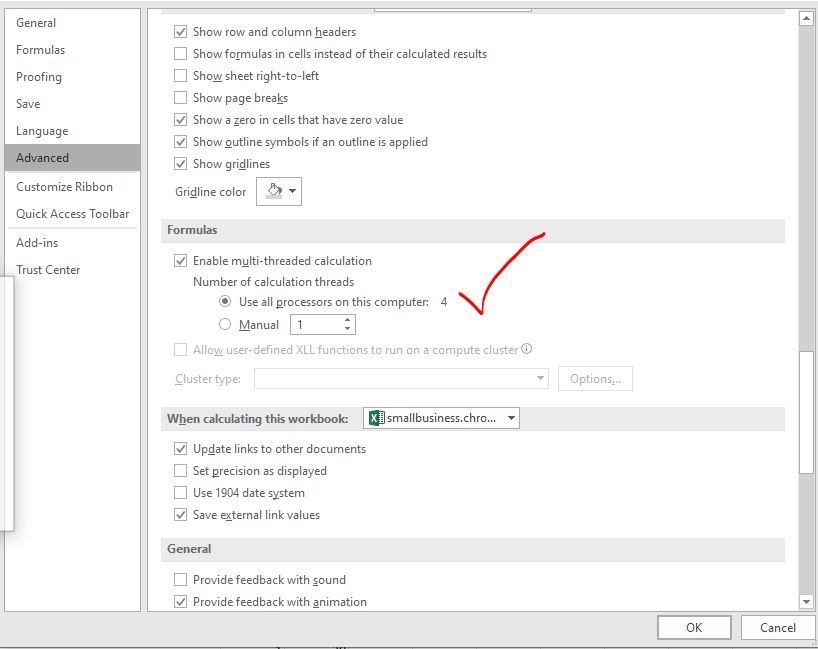
Now excel calculating using 4 processors on my system. It can be more or less on your system.
3: Avoid use of Volatile Functions
The volatile functions like NOW(), OFFSET(), RAND(), etc. recalculate every-time a change is made in Excel file. This increases the burden on the processors. When you have a large number of formulas in the workbook and you make any change in the excel file, the whole file starts to recalculate, even if you don’t want it. This can take too much time and even make Excel crash. So if you have a large number of formulas in the excel file make sure they are not volatile functions.
Some commonly used volatile functions are, OFFSET, RAND, NOW, TODAY, RANDBETWEEN, INDIRECT, INFO, CELL.
4: Switch to Manual Calculation in Excel
If you got have large number of complex formulas with or without volatile functions, set the workbook calculation to manual.
This does not mean that you have to do manual calculations. It just mean that you will tell excel when to recalculate the workbook.
By default, Excel is set to automatic calculations. Due to automatic calculations you can see the change in result of a formula when you change the source data, instantly. This slows the Excel speed.
But if you use manual calculation, the change will not reflect instantly. Once you have done all the task in the sheet, you can use F9 key to tell excel to recalculate the workbook. This will save a lot of resource and time.
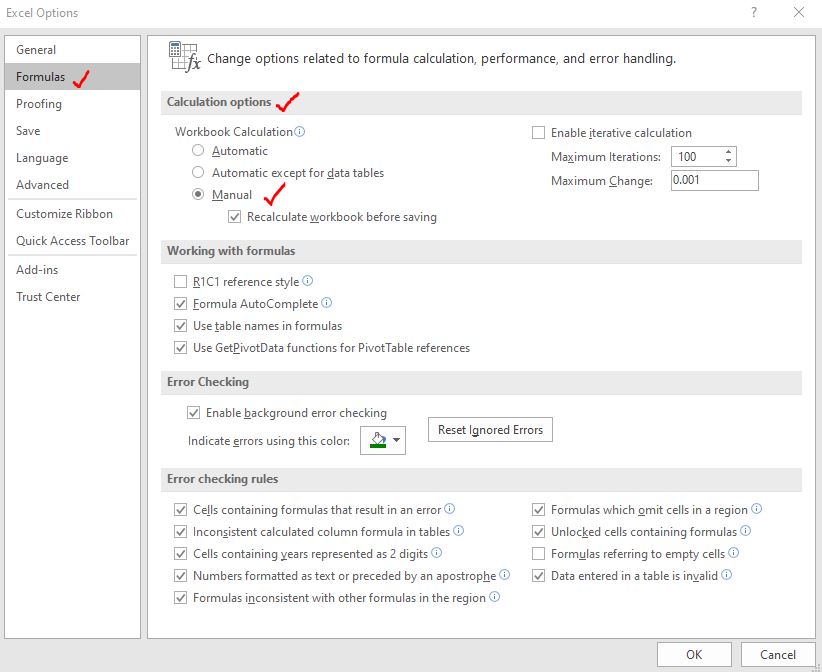
To switch to manual calculations, go to File —> Options —> Formulas. You will have a number of options available. Find calculation option and select the manual calculation and hit the OK button.
5: Do not use Data Tables for Large Data Set
The data tables give a lot functionality that is really helpful. But these functionalities are costly in terms of resources. If you have a large set data than you should avoid using excel data tables. They use a lot of computer resources and can slow down the performance of Excel file. So, if it is not necessary, avoid using Data table for faster calculation of formulas. This will increase formula calculation speed.
6: Replace the Static Formulas with Values:
If you have a large set of calculations and some of the formulas does not change the results, it is better to replace the with values. For example, if you are using VLOOKUP function to import or merge tables for one time, it is better to replace the formula with values.
To do so, copy the result range. Right-Click on the range and go to paste special. Here select Value and hit the OK button. You can read about pasting value here.
7: Disabling the Excel Add ins
The Excel add ins are additional functionalities we add to the tool. They may not needed every time. If you can disable them, you can save a lot of resource on your system. This will help you increase the formula calculation speed.
To disable the add ins go to File —> Options —> Add Ins. Select the add ins and click on Go button.

This will open the add active add ins. Uncheck the add ins that you don’t need. Hit OK button.
This will disable the add ins.
8: Avoid Unnecessary Conditional Formatting in workbook.
The conditional formatting takes a lot of calculation time so it is better to only use them where it is necessary. Do not use the conditional formatting the large data set.
9: Remove unnecessary pivot tables
The pivot tables are great tool for quickly summarizing a large set of data. But if you need the pivot table only for one time, use and delete them. You can keep the value pasted pivot report. If you want to have dynamic data, use formulas.
10: Replace Formulas with VBA Macros
There’s nothing you can’t do using Macros. Sometime it is even more handy and easy to do calculations in VBA than directly on worksheet. You can use the worksheetfunctions object to access the worksheet function VBA. Use them to do large number of calculation and paste value using VBA. This will increase the speed of Excel calculations exponentially.
11: Delete Unused Ranges and Sheets
It is common to use the spare sheets and ranges while working. But you might not know that excel remembers in which ranges you have worked and keeps it into used ranges memory. It is smart delete such sheets and ranges from workbook, so that excel does not uses them any more.
12: Save Excel File as Excel Binary File
If your excel file does not requires to interact with other tools than you should save the excel file as Excel Binary File. The extension of an Excel binary file is .xlsb. This does removes any functionality from excel. Your file just won’t be able to interact with other tools.
13: Consider Using Database tools for storing data.
Most of the time Excel formula calculations slows down due to large amount of data in the workbook. So if you can save the source data in some other database tool or CSV file and use excel for only calculation than you can increase the speed of formula calculations. You can use power pivot or power query to import data temporarily for analyzing data.
So yeah guys, these are the ways to increase the speed of formula calculation in Excel. If you do all these things you will surely increase the calculation speed and excel will not stop or crash while performing calculations.
I hope it was explanatory and helpful. If you have any doubt or special scenario, please let me know in the comments section below. I will be happy to hear from you. Till than keep Excelling.
Related Articles:
Center Excel Sheet Horizontally and Vertically on Excel Page : Microsoft Excel allows you to align worksheet on a page, you can change margins, specify custom margins, or center the worksheet horizontally or vertically on the page. Page margins are the blank spaces between the worksheet data and the edges of the printed page
Split a Cell Diagonally in Microsoft Excel 2016 : To split cells diagonally we use the cell formatting and insert a diagonally dividing line into the cell. This separates the cells diagonally visually.
How do I Insert a Check Mark in Excel 2016 : To insert a checkmark in Excel Cell we use the symbols in Excel. Set the fonts to wingdings and use the formula Char(252) to get the symbol of a check mark.
How to disable Scroll Lock in Excel : Arrow keys in excel move your cell up, down, Left & Right. But this feature is only applicable when Scroll Lock in Excel is disabled.
Scroll Lock in Excel is used to scroll up, down, left & right your worksheet not the cell. So this article will help you how to check scroll lock status and how to disable it?
What to do If Excel Break Links Not Working : When we work with several excel files and use formula to get the work done, we intentionally or unintentionally create links between different files. Normal formula links can be easily broken by using break links option.
Popular Articles:
50 Excel Shortcuts to Increase Your Productivity | Get faster at your task. These 50 shortcuts will make you work even faster on Excel.
How to use Excel VLOOKUP Function| This is one of the most used and popular functions of excel that is used to lookup value from different ranges and sheets.
How to use the Excel COUNTIF Function| Count values with conditions using this amazing function. You don’t need to filter your data to count specific value. Countif function is essential to prepare your dashboard.
How to Use SUMIF Function in Excel | This is another dashboard essential function. This helps you sum up values on specific conditions.
I knew that the performance of M in the query editor of PowerBI was much better than in Excel, but only today I discovered the incredible difference we actually have here:
If you want to apply the BOM-solution I’ve posted here, you’ll soon discover that the performance in Excel starts to suck with large datasets. Performance decreases exponentially and my sample datasets with 4 levels and 100k rows didn’t went through, 16 GB RAM constantly at the limit, unable to do any other task at the same time.
In contrast, performance in PowerBI totally blew me away: Memory management is different. Rise in RAM-consumption was always below 3 GB, even with my largest dataset (a 5-level 1Mio (!) rows BOM table that exploded to 3,8 Mio rows). Also no sweat in CPU, so I was able to easily perform other tasks at the same time on my laptop.
The 100k rows where Excel failed, went through in a good minute, 300k rows BOM exploded in 4 minutes to 1 Mio rows: For a recursive operation (using List.Generate instead of “real recursion”), this is very acceptable in my eyes. 1 Mio rows took a bit under 20 minutes to explode to 3,8 Mio rows.
I must say at I’m really impressed with the performance of PowerBI Desktop with M for a task like this on a PC!
Anyway – if you want to work with the results of your query in Excel (which isn’t so unusual for this kind of data), you have to rely on R for exporting it to csv or SQL-server or use some hacks:
- Access the full datamodel via Pivots
- Import the table via PowerQuery (See in the comment)
Needless to say how much I hope that we wouldn’t need these workarounds. If you agree and want to take some action, please vote for a performance improvement of Power Query in Excel.
Enjoy & stay queryious 😉
Most Excel files are small enough not to affect performance, but size isn’t the only thing that can slow things down. Fortunately, you don’t have to know all about multithreads and dual processors to eliminate bad performance. The following tips are easy to implement, so even the most casual users can improve performance when a workbook slows down. Better yet, apply this advice when designing sheets to help avoid sluggish performance altogether.
1: Work from left to right
This tip is easy to implement because data tends to flow from left to right naturally, but it doesn’t hurt to know that there’s a little more going on under the hood. By default, Excel will calculate expressions at the top-left corner of the sheet first and then continue to the right and down. For this reason, you’ll want to store independent values in the top-left portion of your sheet and enter expressions (dependent cells) to the right or below those values. In a small sheet, you won’t notice much difference, but a sheet with thousands of rows and calculations will definitely perform better when you position dependent cells to the right and below the independent values.
In technical terms, this behavior is called forward referencing. Formulas should be to the right or below the referenced values. Avoid backward referencing, where formulas are to the left and above the referenced values.
2: Keep it all in one sheet
When possible, store everything on the same sheet. It takes longer for Excel to calculate expressions that evaluate values on another sheet. If you’ve already spread your work across several sheets, rearranging everything probably isn’t worth the effort. But keep this one in mind when planning sheets. Keep expressions and references in the same sheet, if possible.
3: Keep it all in the same workbook
Linking to or referencing other workbooks will usually slow things down, even in an uncomplicated workbook. If you can, store everything in the same workbook. Using fewer larger workbooks will be more efficient than using several smaller linked workbooks. When you must use linked workbooks, open them all — and open the linked workbooks before opening the linking workbooks — to improve performance.
4: Clean things up
What you’re not using, delete. Create a backup so you can reclaim functionality at a later date and then delete everything you no longer use. In doing so, you’ll minimize the used range. To determine the used range, press [Ctrl]+[End]. Then, delete all rows and columns below and to the right of your real last used cell. Then, save the workbook.
5: Convert unused formulas
If you’re still referring to derived values (the results of formulas), #4 isn’t feasible. You can, however, convert the formulas to static values. But only do this if you’re sure you will never need to recalculate the formulas that generated the values in the first place. To convert formulas to their static values, use Paste Special and select Values to paste. Doing so will overwrite the formulas with the results of those formulas. Be careful, though. The formulas really will be gone. Create a backup first, just in case.
6: Avoid multiple volatile functions
A volatile function recalculates every time there’s a change in the worksheet, and that slows things down. An efficient alternative is to enter the volatile function by itself and then reference that cell in your formulas. The function will still calculate as expected, but only once instead of hundreds of times. Examples of volatile functions are RAND(), RANDBETWEEN(), NOW(), TODAY(), OFFSET(), CELL(), and INDIRECT().
7: Avoid array formulas
Gurus and power users alike love arrays, and they are a powerful tool. Unfortunately, they’re memory hogs. It might be hard to believe, but a couple of regular formulas will calculate faster than their equivalent array. If helper formulas aren’t adequate, consider a user-defined function. In addition, you might be able to replace arrays with new functions, such as SUMIF(), COUNTIF(), and AVERAGEIF. (Array formulas perform somewhat better in the Ribbon versions of Excel.)
8: Avoid monster formulas
The performance killer in most workbooks is the number of cell reference and operations, not the number of formulas. Throw in some inefficient functions and you can slow things down enough that users will complain. Two or three helper formulas are almost always more efficient than one super colossal formula.
9: Use ISERROR() to update old error-masking formulas
If you’ve upgraded to a Ribbon version of Excel, you can replace most of your convoluted IF() masks with the IFERROR() function:
=IFERROR(expression,actioniferror)This function is more efficient than the pre-Ribbon solution of using IF() in the following form:
=IF(ISERROR(expression),trueaction,falseaction)If you’re still working with a pre-Ribbon version, consider a helper formula (#8). Two columns of simple formulas will be more efficient than a single column of IF() functions.
10: Limit conditional formats
Many techniques rely heavily on conditional formatting, but sometimes at a cost. Every conditional format is evaluated every time the workbook performs calculations. Use conditional formatting wisely, and sparingly. Too many conditional formats will slow things down.
KPI – is the Performance Indicator, which allows objectively evaluates the effectiveness of workflow. This system is used for evaluate of different indicators (the activity throughout the company, separate structures, specific experts). It performs not only control functions, but also stimulates the labor activity. Often based on KPI is based wage system. This is formation technique of the variable part of the salary.
KPI key performance indicators: examples in Excel
The stimulating factor in the system of motivation KPI – is the compensation. To get it may be that an employee, who has fulfilled the task set before him. The prize amount / bonus, depends from the result of a particular employee in the reporting period. The compensation amount may be fixed or be expressed as a percentage of salary.
Each enterprise determines to the key performance indicators and the weight of each individual. Dates are depended from the company’s tasks. For example:
- The purpose — to provide product sales plan of 500 000 rubles monthly. The key performance indicator — is the sales plan. The system of measurement: there are the actual amount of sales / the planned sales amount.
- The task — to increase the amount of shipments in the period by 20%. The key indicator – is the average amount of shipment. The system of measurement: is the actual average value of the shipment / planned average value of the shipment.
- The task — to increase the number of customers by 15% in a particular region. The key indicator – is the number of clients in the company database. The system of measurement: the actual number of customers / the planned number of customers.
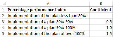
The coefficient of variation (scales), the company also defines by itself. For example:
- The implementation of the plan less than 80% — is unacceptable.
- The implementation of 100% of the plan — the coefficient is 0, 45.
- The implementation of the plan 100 — 115% — the coefficient is 0. 005 for every 5%.
- The absence of errors – the coefficient is 0. 15.
- During the reporting period there were no comments – the coefficient is 0. 15.
This is only the option definition of motivational factors.
The key point in measuring of KPI – is the actual to planned ratios. Almost always the wages of an employee is made up of salary (fixed part) and premium (the variable part /the changeable part). The motivational factor affects the formation of variable part.
Suppose that the ratio of the fixed and the variable parts of the salary — 50 × 50. The Key Performance Indicators and the weight of each of them:
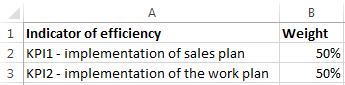
Assume the following meanings of the coefficients (the same ones for 1 indicator and indicator 2):
KPI Table in Excel:
The explanations:
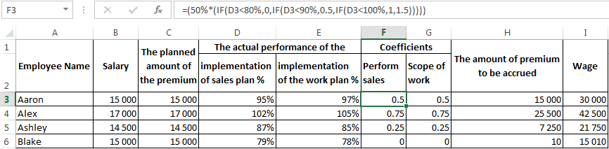
- The salary – is the permanent part of the salary depends on the number of hours worked. For the convenience of calculations we assumed that the fixed and the variable part of the salary are equal.
- The percentage of the sales plan and the work plan are calculated as the ratio of actual performance to planned ones.
- For calculation of the premium are used to the coefficient. The formulas in Excel KPI calculation for each an employee. Perform sales:
Scope of work:
We accepted that the impact of the index 1 and the index 2 for the amount of the premium are the same. The values of the coefficients are also equal. Therefore, for the calculating of the index 1 and the index 2 are used the same formulas (change only the cell references).
- The formula for calculating of the amount of premium to be accrued: =C3*(F3+G3). The planned premium multiplied on the sum of the index 1 and the index 2 for an each employee.
- The wage — salary + premium.
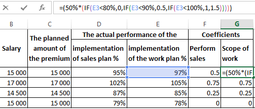
This is the exemplary KPI table in Excel. An each company makes its own a table (with taking into account the characteristics of the work and bonus system).
KPI matrix and the example in Excel
Assessment for employees on the key indicators is compiled the matrix, or an agreement on the objectives. The general form is as follows:
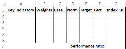
- The key indicators – the criteria for evaluating the work of the staff. They are different for each position.
- The weights – the numbers in the range from 0 to 1, the total sum of which is equaled 1. Reflect the priorities of each the key indicator taking into account the company’s objectives.
- The base – is the allowable minimum value of the index. Following baseline – is not of any result.
- Norma – the planned level. What that an employee must perform necessarily. Below — the employee did not cope with his responsibilities.
- The purpose – is the value for which to aspire. The excess indicator that allows to improve the results.
- The fact – is the actual results.
- The KPI Index shows the level of results in relation to the norm.
The calculation of the formula KPI:
KPI Index = ((Fact — Base) / (Norm — Base)) * 100%.
How to fill in the matrix for an office manager:
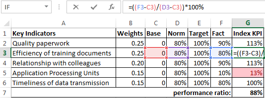
The performance ratio – is the average Index KPI: =AVERAGE(G2:G6). The evaluating of the employee is clearly shown using conditional formatting.

Did you experience a slow workbook? How slow? Let’s say it takes more than 2 minutes to just open the file.
This is actually what a colleague asked me for help. When I opened the workbook, I saw LOTS of SUMIFS across tens of worksheets. And all SUMIFS refer to a common dataset on the workbook.
Then I asked: “Would you consider using Pivot Table instead of so many SUMIFS?”
The answer was “NO” as she needed to use formula to return results that fit into the “pre-set” table layouts, which I totally understood… such a common workplace’s scenario!
Then I proposed GETPIVOTDATA instead of SUMIF(S).
Her responses told me that she didn’t know about GETPIVOTDATA. Maybe I should write a blogpost about GETPIVOTDATA. Before that, let’s test if GETPIVOTDATA is more efficient than SUMIF.
To do the test, I have created two simple columns, with 100,000 rows (large enough to see the time difference) as shown below:

Column A contains 1,000 unique items spread over the range A2:A100001; while Column B are random numbers.
Then on Column E, I generate a list of the first 200 items, i.e. A0000001 to A000200.

On column F, I calculate the total for the (200) items using SUMIF; while on column G, I calculate the same using GETPIVOTDATA.
Let’s see in more details.
In F2:F201, I input the following formula:
=SUMIF($A$2:$A$100001,E2,$B$2:$B$100001)
This is very straight-forward.
In order to use GETPIVOTDATA to obtain the same results as if using SUMIF(s), I have to create a pivot table first.

I inserted the pivot table in J1 on the same worksheet, as shown below:

This pivot table simply summarizes the values of the 1,000 items in the range of A1:B100001
Now, with this pivot table inserted in J1, I would get the following auto-generated GETPIVOTDATA function when I input a = sign in G2 followed by clicking the cell K2. See below:

This formula will look into the “Value” from the pivot table located in $J$1, returning the corresponding item of “A0000001” that is “hard-coded” in the formula. As I need the formula to be copied all the way down to G201, I have to change hard-coded argument into a variable, like this:

In short, I input the following formula into G2:G201:
=GETPIVOTDATA("Value",$J$1,"Item",E2)
Let’s recap what we have prepared so far
- A range of 200 cells using SUMIF
- A range of 200 cells using GETPIVOTDATA via a Pivot Table
Both ranges of data return exactly the same results, i.e. total of the 200 items listed in E2:201 based on the dataset in A2:B100001

To test which function is more efficient, we simply calculate the time required to calculate the range, with the help of some VBA codes. If you are interested in how, take a look at this article. Indeed, I strongly recommend you read the entire article.
Let’s see the result
Five tests were run separately on the range F2:F201 and G2:201, where SUMIF and GETPIVOTDAT is used respectively.
Here’s the result for SUMIF: On average it takes 0.76 second.

Here’s the result for GETPIVOTDATA: On average it takes 0.017 second.

0.76s vs. 0.017s…
K.O.
GETPIVOTDATA runs 40+ times faster than SUMIF in this scenario.
Why is that?
I am not an expert in performance optimization nor do I have the technical knowledge to answer this question. My wild guess is the huge number of cells involved in the two functions. Think about the case for SUMIF, each formula looks into a range of 100,000 cells; while for GETPIVOTDATA, each formula looks into only 1,000 cells. Is that a big difference already?
Having said that, there is one major drawback using GETPIVOTDATA. The result is not instantly recalculated with updates. See below:

When the data source is updated, SUMIF recalculates instantly. However, the result returned by GETPIVOTDATA remains unchanged until the related pivot table has got refreshed, manually.
At this point, you may be thinking… that’s not ideal. No, it is not. But think twice. For a slow workbook because of lots of inefficient formulas, you would probably turn the calculation option to manual; and every time you need updated results, you have to press F9 to recalculate. IF this is what you are doing, I’d say GETPIVOTDATA wins. 😉
Conclusion:
GETPIVOTDATA can be much more efficient than SUMIF(s). Although it’s not perfect, it would be a good alternative to tones of expensive formulas like SUMIF(S).
In case you would like to do the test by yourself, you may download the sample file.
Skip to content
My posts from two weeks ago (see here and here) on using Process Monitor to troubleshoot the performance of Power Query queries made me wonder about another question: how does the performance of reading data from CSV files compare to the performance of reading data from Excel files? I think most experienced Power Query users in either Power BI or Excel know that Excel data sources perform pretty badly but I had never done any proper tests. I’m not going to pretend that this post is a definitive answer to this question (and once again, I would be interested to hear your experiences) but hopefully it will be thought-provoking.
To start off, I took the 153.6MB CSV file used in my last few posts and built a simple query that applied a filter on one text column, then removed all but three columns. The query ran in 9 seconds and using the technique from my last post I was able to draw the following graph from a Process Monitor log file showing how Power Query reads data from the file:

Nothing very surprising there. Then I opened the same CSV file in Excel and saved the data as an xlsx file with one worksheet and no tables or named ranges; the resulting file was only 80.6MB. Finally I created a duplicate of the first query and pointed it to the Excel file instead. The resulting query ran in 59 seconds – around 6 times slower! Here’s a comparison with the performance of this query with the first query:

The black line in the graph above is the amount of data read (actually the offset values showing where in the file the data is read from, which is the same thing as a running total when Power Query is reading all the data) from the Excel file; the green line is the amount of data read from the CSV file (the same data shown in the first graph above). A few things to mention:
- Running Process Monitor while this second query was refreshing had a noticeable impact on its performance – in fact it was almost 20 seconds slower
- The initial values of 80 million bytes seem to be where data is read from the end of the Excel file. Maybe this is Power Query reading some file metadata? Anyway, it seems as though it takes 5 seconds before it starts to read the data needed by the query.
- There’s a plateau between the 10 and 20 second mark where not much is happening; this didn’t happen consistently and may have been connected to the fact that Process Monitor was running
In any case you don’t need to study this too hard to understand that the performance of reading data from an xlsx format Excel file is terrible compared to the performance of reading data from a CSV. So, if you have a choice between these two formats, for example when downloading data, it seems fair to say that you should always choose CSV over xlsx.

My name is Chris Webb, and I work on the Power BI CAT team at Microsoft. I blog about Power BI, Power Query, SQL Server Analysis Services, Azure Analysis Services and Excel.
View all posts by Chris Webb