
I have two columns in Excel, and I want to find (preferably highlight) the items that are in column B but not in column A.
What’s the quickest way to do this?
![]()
Excellll
12.5k11 gold badges50 silver badges78 bronze badges
asked Dec 10, 2009 at 18:44
![]()
- Select the list in column A
- Right-Click and select Name a Range…
- Enter «ColumnToSearch»
- Click cell C1
- Enter this formula:
=MATCH(B1,ColumnToSearch,0) - Drag the formula down for all items in B
If the formula fails to find a match, it will be marked #N/A, otherwise it will be a number.
If you’d like it to be TRUE for match and FALSE for no match, use this formula instead:
=ISNUMBER(MATCH(B1,ColumnToSearch,0))
If you’d like to return the unfound value and return empty string for found values
=IF(ISNUMBER(MATCH(B1,ColumnToSearch,0)),"",B1)
![]()
answered Dec 10, 2009 at 19:01
![]()
devuxerdevuxer
3,9316 gold badges31 silver badges33 bronze badges
6
Here’s a quick-and-dirty method.
Highlight Column B and open Conditional Formatting.
Pick Use a formula to determine which cells to highlight.
Enter the following formula then set your preferred format.
=countif(A:A,B1)=0
![]()
Excellll
12.5k11 gold badges50 silver badges78 bronze badges
answered May 9, 2011 at 16:18
![]()
EllesaEllesa
10.8k2 gold badges38 silver badges52 bronze badges
2
Select the two columns. Go to Conditional Formatting and select Highlight Cell Rules. Select Duplicate values. When you get to the next step you can change it to unique values. I just did it and it worked for me.
answered Apr 16, 2015 at 20:02
![]()
DOB DOB
2813 silver badges2 bronze badges
4
Took me forever to figure this out but it’s very simple. Assuming data begins in A2 and B2 (for headers) enter this formula in C2:
=MATCH(B2,$A$2:$A$287,0)
Then click and drag down.
A cell with #N/A means that the value directly next to it in column B does not show up anywhere in the entire column A.
Please note that you need to change $A$287 to match your entire search array in Column A. For instance if your data in column A goes down for 1000 entries it should be $A$1000.
![]()
n.st
1,8781 gold badge17 silver badges30 bronze badges
answered Dec 6, 2013 at 20:43
![]()
brentonbrenton
1711 silver badge2 bronze badges
1
See my array formula answer to listing A not found in B here:
=IFERROR(INDEX($A$2:$A$1999,MATCH(0,IFERROR(MATCH($A$2:$A$1999,$B$2:$B$399,0),COUNTIF($C$1:$C1,$A$2:$A$1999)),0)),»»)
Comparing two columns of names and returning missing names
![]()
C. Ross
6,06416 gold badges60 silver badges82 bronze badges
answered Oct 21, 2011 at 14:02
![]()
1
My requirements was not to highlight but to show all values except that are duplicates amongst 2 columns. I took help of @brenton’s solution and further improved to show the values so that I can use the data directly:
=IF(ISNA(MATCH(B2,$A$2:$A$2642,0)), A2, "")
Copy this in the first cell of the 3rd column and apply the formula through out the column so that it will list all items from column B there are not listed in column A.
answered Feb 24, 2014 at 11:10
![]()
1
Thank you to those who have shared their answers. Because of your solutions, I was able to make my way to my own.
In my version of this question, I had two columns to compare — a full graduating class (Col A) and a subset of that graduating class (Col B). I wanted to be able to highlight in the full graduating class those students who were members of the subset.
I put the following formula into a third column:
=if(A2=LOOKUP(A2,$B$2:$B$91),1100,0)
This coded most of my students, though it yielded some errors in the first few rows of data.
answered Sep 11, 2014 at 13:25
![]()
in C1 write =if(A1=B1 , 0, 1). Then in Conditional formatting, select Data bars or Color scales. It’s the easiest way.
![]()
Jawa
3,60913 gold badges31 silver badges36 bronze badges
answered Feb 16, 2015 at 9:52
![]()
VBA question: I have two columns in excel:
A   B
10  6
5   1
6   4
2   7
8   9
4   8
9   10
7   5
    3
    11
Now I need the result to contain those value which are in column B, but not in column A. I know that I can use CountIf to solve the problem. However, is there any way that I can do it in VBA without looping?
![]()
BoffinBrain
6,2376 gold badges33 silver badges59 bronze badges
asked Sep 26, 2017 at 7:33
![]()
3
Try with Below Formula,
in D2 place the below formula, select D2 to D11 and Press CTRL+D.
=IF(ISNA(MATCH(B2,A:A,0))=TRUE,B2 & " Not Exist in Column A", B2 & " Exist in Column A")
OP

answered Sep 26, 2017 at 8:26
![]()
Try this:
Sub Demo()
    Dim ws As Worksheet
    Dim cel As Range, rngA As Range, rngB As Range
    Dim lastRowA As Long, lastRowB As Long
    Application.ScreenUpdating = False

    Set ws = ThisWorkbook.Sheets("Sheet3")  'change Sheet3 to your data range

    With ws
        lastRowA = .Cells(.Rows.Count, "A").End(xlUp).Row   'last row with data in Column A
        lastRowB = .Cells(.Rows.Count, "B").End(xlUp).Row   'last row with data in Column B
        Set rngA = .Range("A2:A" & lastRowA)                 'range with data in Column A
        Set rngB = .Range("B2:B" & lastRowB)                 'range with data in Column B

        .Range("C2").Formula = "=IF(COUNTIF(" & rngA.Address & ",$B2)=0,B2,"""")"   'enter formula in Cell C2
        .Range("C2").AutoFill Destination:=.Range("C2:C" & lastRowB)                'drag formula down
        .Range("C2:C" & lastRowB).Value = .Range("C2:C" & lastRowB).Value           'keep only values
        .Range("C2:C" & lastRowB).SpecialCells(xlCellTypeBlanks).Delete Shift:=xlUp 'delte blank rows
    End With
    Application.ScreenUpdating = True
End Sub

answered Sep 26, 2017 at 7:48
![]()
MrigMrig
11.6k2 gold badges13 silver badges27 bronze badges
3
Just for fun (and speed), you can also do that with SQL :
Sub SqlSelectExample()
'list elements in col C not present in col B
    Dim con As ADODB.Connection
    Dim rs As ADODB.Recordset
    Set con = New ADODB.Connection
    con.Open "Driver={Microsoft Excel Driver (*.xls)};" & _
           "DriverId=790;" & _
           "Dbq=" & ThisWorkbook.FullName & ";" & _
           "DefaultDir=" & ThisWorkbook.FullName & ";ReadOnly=False;"
    Set rs = New ADODB.Recordset
    rs.Open "select ccc.test3 from [Sheet1$] ccc left join [Sheet1$] bbb on ccc.test3 = bbb.test2 where bbb.test2 is null  ", _
            con, adOpenStatic, adLockOptimistic
    Range("g10").CopyFromRecordset rs   '-> returns values without match
    rs.MoveLast
    Debug.Print rs.RecordCount          'get the # records
    rs.Close
    Set rs = Nothing
    Set con = Nothing
End Sub
You will have to rework the SQL a bit.
answered Sep 26, 2017 at 9:02
![]()
iDevlopiDevlop
24.6k11 gold badges89 silver badges147 bronze badges
2
![]()
level 1
Mod · 2 yr. ago · Stickied commentLocked
/u/horriblethinker — please read this comment in its entirety.
Once your problem is solved, please reply to the answer(s) saying Solution Verified to close the thread.
Please ensure you have read the rules — particularly 1 and 2 — in order to ensure your post is not removed.
I am a bot, and this action was performed automatically. Please contact the moderators of this subreddit if you have any questions or concerns.
level 1
If I’m understanding you right, you just want to make sure both columns contain the exact same list of account numbers, right?
A simple way is to use conditional formatting. Select the two columns. Go to highlight cells rules, click on duplicate values. Click on the duplicates dropdown and change it to unique. That’ll highlight every unique value in the two rows so you will be able to tell if there are some in one column that aren’t in the other. I don’t know how big of a data set you are working with but that will tell you if there are some missing.
level 2
That is exactly what I’m trying to do. I need to figure out how to do that though. I’ve never seen»highlight cell rules» before though.
level 2
I have to say thank you so much. I got it to do exactly what I needed! I am so glad I asked instead of letting this take me weeks to do. Thank you!!!
level 1
=countif(column1, cell 1 in column2)
Lock column 1 reference then drag down formula.
It will tell you which cells in column 2 don’t exist in column 1
level 1
With data in columns A & B
C2 =IF(MATCH(B2,$A$2:$A$2001,0),1) and filldown
If the same in both, 1 or #N/A if not.
EDIT: Typo D instead of A
level 2
Samedi system =if(count if(b:b;a2) >1)
Or without the if so you can identify doubles, triples etc.
level 1
If they are just numbers, subtract one column from the other and any nonzero values will show you the unique values.
level 1
In a corresponding 3rd column use the formula =IF(column1=column2,”Good”,”Error”) and copy/drag all the way down.
Then you can use the third column (by filtering for “Error”) to see which rows do not match.
level 1
Personally, I’d use PowerQuery/Get & transform.
Load both list as connection only. Then perform one of following joins (merge operation).
-
Left Anti — This will show items present in left side, that isn’t present on right side.
-
Right Anti — This will show items present in right side, that isn’t present on left side.
-
Full outer — It will show null for value not present on each side.
Use one that suite your need.
Alternate approach is to use data relationship. Assuming account number is unique.
level 1
i just do this old school. Create a column with the information from the 1st column (starting in a1 as an example), past the information from the 2nd column next to that, in the 3rd column put the formula a1=b1. filter this looking for the falses
level 2
I can’t do that because none of the numbers would match since each column is missing numbers. I am in the process of doing this and it’s taking forever, looking for the missing ones on each side. I have 28,000 numbers and there’s around 5,000 missing total so I need something quicker.
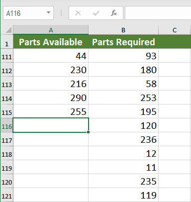
What I want to do
Find Items in one column (ColA) that are not in another column (ColB). What to do when I want the result not being highlighted, but have it in another column (ColC) without blank rows.
Example
ColA - ColB - ColC
1 - 1 - 4
3 - 2 - 8
10 - 3 - 10
4 - 5 - ""
5 - 7 - ""
8 - 6 - ""
9 - 9 - ""
What did I try yet
Until now I succeeded to have the following result. I do this with the following formula in column C:
=IF(IFERROR(MATCH(A2;B$2:F$300;0);"")<>"";"";A2)
Result:
ColA - ColB - ColC
1 - 1 - ""
3 - 2 - ""
10 - 3 - 10
4 - 5 - 4
5 - 7 - ""
8 - 6 - 8
9 - 9 - ""
But I want to avoid the blank cells in Col C.
I tried the formula I found in one of the answers on this site:
IFERROR(INDEX($A$2:$A$1999,MATCH(0,IFERROR(MATCH($A$2:$A$1999,$B$2:$B$399,0),COUNTIF($C$1:$C1,$A$2:$A$1999)),0)),"")
… but this does not work. Maybe I adapt this formula in a wrong way…?
When you need to check if one column value exists in another column in Excel, there are several options. One of the most important features in Microsoft Excel is lookup and reference. The VLOOKUP, HLOOKUP, INDEX and MATCH functions can make life a lot easier in terms of looking for a match.
In this tutorial, we will see the use of VLOOKUP and INDEX/MATCH to check if one values from one column exist in another column.
Check if one column value exists in another column
In the following example, you will work with automobile parts inventory data set. Column A has the parts available, and column B has all the parts needed. Column A has 115 entries, and column B has 1001 entries. We will discuss a couple of ways to match the entries in column A with the ones in column B. Column C will output “True” if there is a match, and “False” if there isn’t.
Check if one column value exists in another column using MATCH
You can use the MATCH() function to check if the values in column A also exist in column B. MATCH() returns the position of a cell in a row or column. The syntax for MATCH() is =MATCH(lookup_value, lookup_array, [match_type]). Using MATCH, you can look up a value both horizontally and vertically.
Example using MATCH
To solve the problem in the previous example with MATCH(), you need to follow the following steps:
- Select cell C2 by clicking on it.
- Insert the formula in
"=NOT(ISERROR(MATCH(A2,$B$2:$B$1001,0)))”the formula bar. - Press Enter to assign the formula to C2.

- Drag the formula down to the other cells in column C clicking and dragging the little “+” icon on the bottom-right of C2.
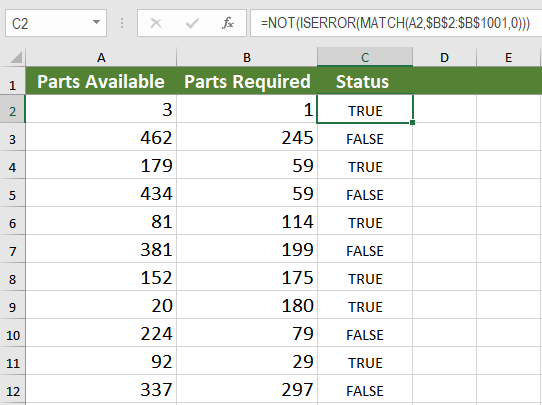
Excel will match the entries in column A with the ones in column B. If there is a match, it will return the row number. The NOT() and ISERROR() functions check for an error which would be and column C will show “True” for a match and “False” if it is not a match.
Check if one column value exists in another column using VLOOKUP
VLOOKUP is one of the lookup, and reference functions in Excel and Google Sheets used to find values in a specified range by “row.” It compares them row-wise until it finds a match. In this tutorial, we will look at how to use VLOOKUP on multiple columns with multiple criteria. The syntax for VLOOKUP is =VLOOKUP(value, table_array, col_index,[range_lookup]).
Example using VLOOKUP
You can check if the values in column A exist in column B using VLOOKUP.
- Select cell C2 by clicking on it.
- Insert the formula in
“=IF(ISERROR(VLOOKUP(A2,$B$2:$B$1001,1,FALSE)),FALSE,TRUE)”the formula bar. - Press Enter to assign the formula to C2.
- Drag the formula down to the other cells in column C clicking and dragging the little “+” icon on the bottom-right of C2.
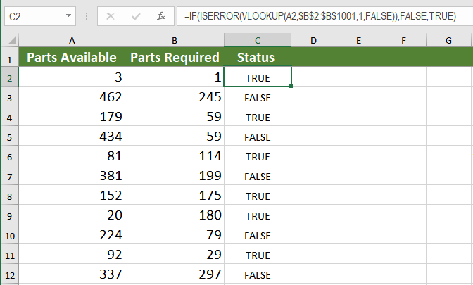
This will allow Excel to look up all the values in column A and match them with the values of column B. Column C will now show “True” if the corresponding cell in column A has a match in column B, “False” if it does not have a match.
MATCH vs. VLOOKUP – Which is Better?
Between MATCH and VLOOKUP, the better option is MATCH. Not only the formula is simpler, but MATCH is also faster than VLOOKUP when it comes to performance.
MATCH uses a dynamic column reference whereas VLOOKUP uses a static one. If you were to add more columns, with VLOOKUP, you would distort the results. But with MATCH you can easily change the reference when inserting or deleting columns.
Another issue with VLOOKUP is that the lookup value needs to be on the leftmost column of the array, which is not applicable for MATCH. In the previous example, If we had to check if Column C values exist in column A, VLOOKUP would have provided an #N/A error.
Excel has some very effective functions when it comes to checking if values in one column exist in another column. One of these functions is MATCH. It returns the row number based on the lookup value from an array. Another such function is VLOOKUP. It returns the value based on a lookup value from a static array.
When it comes to which function is faster, MATCH is the winner. For its dynamic reference and easy to change array references, MATCH is preferred to check if values in one column also exist in another column.
Most of the time, the problem you need is probably more complex than just simply checking if a value exists in a column. If you want to save hours of researching and frustration, try our Excel Live Chat service! Our Excel experts are available 24/7 to answer any Excel question you have on the spot. The first question is free.
Are you still looking for help with the VLOOKUP function? View our comprehensive round-up of VLOOKUP function tutorials here.
One of the best things about Microsoft Excel is that it can be customized to suit your needs and preferences.
Excel has Conditional Formatting that allows you to format a cell based on the value in it. But with a little bit of formula magic, you can also highlight a cell or range of cells based on whether a value exists in some other columns or not.
For example, if you have a dataset with a person’s name and their country, and you want to highlight all the names that are from the US, you can easily do that using conditional formatting.
In this tutorial, I will show you how to highlight a cell or range of cells if the value exists in another column in Excel.
So, let’s get started!
Highlight Cells Based on Value in Another Column
Suppose you have a data set as shown below and you want to highlight all the names in column A if the country in column B is ‘US’.

Below are the steps to do this using Conditional Formatting:
- Select the column in which you want to highlight the cells (the Names column in our example)
- Click the Home tab

- In the Styles group, click on Conditional Formatting

- In the options that show up, click on the New Rule option. This will open the New Formatting Rules dialog box

- In the ‘Select a Rule type’ options, click on ‘Use a formula to determine which cells to format’

- Enter the following formula in the field below: =B2=”US”

- Click on the Format button
- In the Fill tab, choose the color in which you want to highlight the cells

- Click OK
- Click OK


The above steps would highlight only those names where the country in the adjacent column is the US.

Note that in this example, I have hard-coded the country name in the formula (=B2=”US”). in case you have the country name in a cell, you can also use the reference of the cell instead of using the exact name.
How Does this Work?
When you select a range of cells and apply conditional formatting on it, Excel would go through each of the cells in the selected range and check it using the condition that you have specified (which in our case was the formula =B2=”US”)
When it analyzes cell A2, it checks whether the formula would return True or not. So, it would check cell B2 and see if the value is equal to the US or not.
If the formula returns True, then the cell in column a would get highlighted with the specified format. And if the formula turns FALSE, then nothing would happen.
Similarly, it keeps analyzing all the cells in the Names column and highlights all those where the country name in column B is the US.
Highlight Entire Rows Based on Value in One Column
Another scenario where you can use the same concept is when you want to highlight the entire row based on the value in any one column.
For example, suppose you have a data set as shown below and you want to highlight all the records where the country is ‘US’
We can use a similar concept as we used in the example above, but instead of applying conditional formatting to one column, we’ll have to apply it to the entire data set.
Below are the steps to do this:
- Select the entire dataset
- Click the Home tab
- In the Styles group, click on Conditional Formatting
- In the options that show up, click on the New Rule option. This will open the New Formatting Rules dialog box
- In the ‘Select a Rule type’ options, click on ‘Use a formula to determine which cells to format’
- Enter the following formula in the field below: =$B2=”US”
- Click on the Format button
- In the Fill tab, choose the color in which you want to highlight the cells
- Click OK
- Click OK
The above steps would highlight all those records where the country in column B is ‘US’

How Does this Work?
When you select a range of cells (including multiple rows and columns), conditional formatting would go through each cell and check the result of the formula that you have specified.
If the result is TRUE, it would highlight the cell, and if the result is FALSE then it would do nothing.
In our example, I would like to highlight all the cells in a row where the country in column B is the US.
This means that no matter what cell is being analyzed in a row, the formula that needs to be analyzed should always check whether the country is the US or not.
And this is done using the below formula:
=$B2="US"
By adding a dollar sign before the column letter B, I have made this a mixed reference. this means that no matter which sale is being analyzed in the row, conditional formatting would always check the cell value in column B and see if that is equal to the US or not.
So when cell A2 is analyzed by conditional formatting, it checks whether the value in B2 is the US or not. and then cell B2 is analyzed, it does the same.
And now when cell A3 is analyzed by conditional formatting, it would check the country name in cell B3, and so on.
This is how you can highlight cells in Excel based on whether the value exists in another cell or not. and you can also highlight an entire record based on the value in one specific column.
I hope you found this tutorial useful.
Other Excel tutorials you may also like:
- How to Highlight Every Other Row in Excel (Conditional Formatting & VBA)
- How to Find Duplicates in Excel (Conditional Formatting/ Count If/ Filter)
- How to Hide Rows based on Cell Value in Excel
- Using Conditional Formatting with OR Criteria in Excel
- How to Copy Formatting In Excel
- How to Highlight Blank Cells in Excel? 3 Easy Methods!
- How to Change Font Color Based on Cell Value in Excel?
Example: Compare Two Columns and Highlight Mismatched Data
- Select the entire data set.
- Click the Home tab.
- In the Styles group, click on the ‘Conditional Formatting’ option.
- Hover the cursor on the Highlight Cell Rules option.
- Click on Duplicate Values.
- In the Duplicate Values dialog box, make sure ‘Unique’ is selected.
How do I combine two date columns in Excel?
- BUT….
- Step 1: Here is the simple formula to combine Date & Time in Excel.
- Step 2: A2 indices the first date in Date Column & B2 is for Time Column.
- Step 3: Type this formula = TEXT(A2,”m/dd/yy “)EXT(B2,”hh:mm:ss”) into next column.
- Step 4: Now you will get Combine Date & Time in Excel.
How do I merge two columns in Excel and keep all data?
Combine data with the Ampersand symbol (&)
- Select the cell where you want to put the combined data.
- Type = and select the first cell you want to combine.
- Type & and use quotation marks with a space enclosed.
- Select the next cell you want to combine and press enter. An example formula might be =A2&” “&B2.
How do I combine two columns in matching tables?
Combine tables in Excel by column headers
- On your Excel ribbon, go to the Ablebits tab > Merge group, and click the Combine Sheets button:
- Select all the worksheets you want to merge into one.
- Choose the columns you want to combine, Order ID and Seller in this example:
- Select additional options, if needed.
How do I combine multiple worksheets into one?
On the Excel ribbon, go to the Ablebits tab, Merge group, click Copy Sheets, and choose one of the following options:
- Copy sheets in each workbook to one sheet and put the resulting sheets to one workbook.
- Merge the identically named sheets to one.
- Copy the selected sheets to one workbook.
How do I put two tables next to each other in Word?
You can insert two or more tables next to each other in Microsoft Word 2016: all you have to do is drag-and-drop them to any part of the document.
Can we join two tables without any relation?
The answer to this question is yes, you can join two unrelated tables in SQL and in fact, there are multiple ways to do this, particularly in the Microsoft SQL Server database. The most common way to join two unrelated tables is by using CROSS join, which produces a cartesian product of two tables.
Can we join two tables without common columns?
Yes, you can! The longer answer is yes, there are a few ways to combine two tables without a common column, including CROSS JOIN (Cartesian product) and UNION. The latter is technically not a join but can be handy for merging tables in SQL.
How do I get two columns from different tables in SQL?
Example syntax to select from multiple tables:
- SELECT p. p_id, p. cus_id, p. p_name, c1. name1, c2. name2.
- FROM product AS p.
- LEFT JOIN customer1 AS c1.
- ON p. cus_id=c1. cus_id.
- LEFT JOIN customer2 AS c2.
- ON p. cus_id = c2. cus_id.
Which join is based on all columns in the two tables that have the same column name?
NATURAL JOIN
How can I put two table data in one query?
Different Types of SQL JOINs
- (INNER) JOIN : Returns records that have matching values in both tables.
- LEFT (OUTER) JOIN : Returns all records from the left table, and the matched records from the right table.
- RIGHT (OUTER) JOIN : Returns all records from the right table, and the matched records from the left table.
Why we create multiple tables in database?
Basically a single table is good when data is one-to-one. When you have thousands of rows and columns of data, where the data is one-to-many, multiple tables are better to reduce duplicate data.
How do you update a field from another table in access?
Use a Field in One Table to Update a Field in Another Table
- Create a standard Select query.
- Select Query → Update to change the type of query to an update action query.
- Drag the field to be updated in the target table to the query grid.
- Optionally specify criteria to limit the rows to be updated.
How do I move data from one table to another in access?
Copy an existing table structure into a new Access database
- Right-click the existing table name in the Database Window of the original database and click Copy.
- Close the database Window and open your new database.
- Under Objects, click Tables. Then, right-click the database Window and click Paste.
- Enter a name for the new table, choose Structure Only, and then click OK.
What is the difference between a one-to-one join and a one-to-many join?
One-to-one relationships associate one record in one table with a single record in the other table. One-to-many relationships associate one record in one table with many records in the other table.
What is the difference between one-to-one and one-to-many relationship?
A one-to-one relationship is created if both of the related fields are primary keys or have unique indexes. A many-to-many relationship is really two one-to-many relationships with a third table whose primary key consists of two fields ï¿ the foreign keys from the two other tables.
What is this relationship called can be a one-to-one one-to-many many to one or many-to-many relationship?
This type of relationship can be created using Primary key-Foreign key relationship. This kind of Relationship, allows a Car to have multiple Engineers.
Can you have a many to one relationship?
For example, if one department can employ for several employees then, department to employee is a one to many relationship (1 department employs many employees), while employee to department relationship is many to one (many employees work in one department). Most relations between tables are one-to-many.
What is the kind of relationship between ω and ω many to one one to many one-to-one many-to-many?
The frequency mapping is not aliased; that is, the relationship between Ω and ω is one-to-one.
What are the 3 types of relation?
The types of relations are nothing but their properties. There are different types of relations namely reflexive, symmetric, transitive and anti symmetric which are defined and explained as follows through real life examples.
Are you having difficulty merging two or more Excel columns? Knowing how to combine multiple columns in Excel without losing data is a handy time-saver that allows you to consolidate your data and make your sheet look neater.
First and foremost, you should know that there are multiple ways you can merge data from two or more columns in Excel. Before we get started exploring these different ways, let’s start with a key step that helps the process — how to merge cells in Excel.
If you want to combine Google Sheets data, you can do that easily using Layer. Layer is a free add-on that allows you to share sheets or ranges of your main spreadsheet with different people. On top of that, you get to monitor and approve edits and changes made to the shared files before they’re merged back into your master file, giving you more control over your data.
Install the Layer Google Sheets Add-On today and Get Free Access to all the paid features, so you can start managing, automating, and scaling your processes on top of Google Sheets!
How to Combine Multiple Cells or Columns in Excel Without Losing Data?
Once you have merging cells under your belt, learning how to combine multiple Excel columns into one column becomes intuitive.
Whether you’re learning how to combine two cells in Excel, or ten, one of the main benefits of merging is that the formulae don’t change. Here are the following ways you can combine cells or merge columns within your Excel:
Use Ampersand (&) to merge two cells in Excel
If you want to know how to merge two cells in Excel, here’s the quickest and easiest way of doing so without losing any of your data.
- 1. Double-click the cell in which you want to put the combined data and type =
- 2. Click a cell you want to combine, type &, and click the other cell you wish to combine. If you want to include more cells, type &, and click on another cell you wish to merge, etc.
- 3. Press Enter when you have selected all the cells you want to combine

While this is useful for quickly merging data into a single cell, the merged data will not be formatted. This can make data untidy or challenging to read in some instances (e.g. full names or addresses).
If you want to add punctuation or spaces (delimiters), follow the below steps. For this example, let’s put a comma and a space between the first and last name as you would see on a registration list:
- 1. Double-click the cell in which you want to put the merged data and type =
- 2. Click a cell you want to merge
- 3. This time, type &”, ”& before you click the next cell you want to merge. If you want to include more cells, type &”, ”& before clicking the next cell you want to merge, etc.
- 4. Press Enter when you have selected all the cells you want to combine

As you can see, now your merged data comes out in a neater format, with each piece of data appropriately separated.
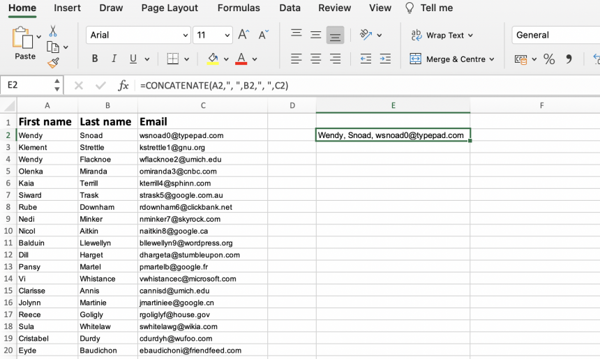
Use the CONCATENATE function to merge multiple columns in Excel
This method is similar to the ampersand method, and also allows you to format your merged data. First, you need to use the CONCATENATE function to merge a row of cells:
- 1. Insert the =CONCATENATE function as laid out in the instructions above
- 2. Type in the references of the cells you want to combine, separating each reference with ,», «, (e.g. B2,», «,C2,», «,D2). This will create spaces between each value.
- 3. Press Enter
Now that you have successfully merged your cells, you can follow these simple steps to merge multiple columns:
- 1. Hover your mouse over the bottom-right corner of the merged cell you just created
- 2. When the cursor changes into a + symbol, drag your cursor as far down the column as you want and release it

Once you release the mouse, you should see that your merged cell has become a merged column, containing all of the data from your chosen columns.
*The CONCAT function is another formula used for combining data from different cells. However, it is limited to two references and does not allow you to include delimiters.
Use the TEXTJOIN function to merge multiple columns in Excel
This method works only with Excel 365, 2021, and 2019. As you can probably tell, this function is helpful when you want to combine two or more text cells in Excel.
The following steps will show you how to use the TEXTJOIN function, once again using the comma and space combination to create your first merged cell:
- 1. Double-click the cell in which you want to put the combined data
- 2. Type =TEXTJOIN to insert the function
- 3. Type “, ”,TRUE, followed by the references of the cells you want to combine, separating each reference with a comma (the role of TRUE is to disregard empty cells you may have input)
- 4. Press Enter

In order to create the rest of your combined column, use the drag-and-drop steps listed below:
- 1. Hover your mouse over the bottom-right corner of the merged cell you just created
- 2. When the cursor changes into a + symbol, drag your cursor as far down the column as you want and release it.

Now your columns of data have successfully merged into your new column.
The Beginner’s Guide to Excel Version Control
Discover what Excel version control is, the version control features Excel has to offer, and how to use them to share, merge, and review Excel changes
READ MORE

Use the INDEX formula to stack multiple columns into one column in Excel
Let’s say you want to create a stack of data from your multiple columns, rather than create a single cell. You can easily do this across multiple cells and columns within your spreadsheet using the INDEX formula:
- 1. Select all of the cells containing your data
- 2. Type in a name for this group of data in the “Name Box” (box located to the left side of the formula bar). In this example, I’ve named the data “_my_data”
- 3. Select an empty cell in your Excel sheet where you want your stacked data to be located. Input the following INDEX formula (remember to substitute with your data name):
=INDEX(_my_data,1+INT((ROW(A1)-1)/COLUMNS(_my_data)),MOD(ROW(A1)-1+COLUMNS(_my_data),COLUMNS(_my_data))+1)
-
4. The first value from your data range should appear. Hover over the cell until the cursor changes into a + symbol, and drag your cursor as far down until you receive a #REF! value (this signals the end of your data set)

Other ways to combine multiple columns in Excel: Notepad and VBA script
There are two other ways you can combine multiple columns in Excel. These are often more time-consuming, and use other tools as part of the process. However, they may be more helpful for users who wish to avoid using Excel formulae.
Use Notepad to merge multiple columns in Excel
You can use Notepad to extract, format, and replace your data from multiple columns in your Excel. For this, you need to copy and paste each column from your Excel sheet into a Notepad file. Then, use the Replace function to add commas between each value. Once finished, you can copy and paste your formatted data back into your Excel.
Use VBA script to combine two or more columns in Excel
As an alternative to the INDEX function stacking method, you can use VBA script. Simply right-click and select “View code” within your Excel, and copy and paste the code in a new window. Press “F5” to run the code and create a Macro. You can then apply this to your Excel by selecting your data range and applying it to your destination column.
Want to Boost Your Team’s Productivity and Efficiency?
Transform the way your team collaborates with Confluence, a remote-friendly workspace designed to bring knowledge and collaboration together. Say goodbye to scattered information and disjointed communication, and embrace a platform that empowers your team to accomplish more, together.
Key Features and Benefits:
- Centralized Knowledge: Access your team’s collective wisdom with ease.
- Collaborative Workspace: Foster engagement with flexible project tools.
- Seamless Communication: Connect your entire organization effortlessly.
- Preserve Ideas: Capture insights without losing them in chats or notifications.
- Comprehensive Platform: Manage all content in one organized location.
- Open Teamwork: Empower employees to contribute, share, and grow.
- Superior Integrations: Sync with tools like Slack, Jira, Trello, and more.
Limited-Time Offer: Sign up for Confluence today and claim your forever-free plan, revolutionizing your team’s collaboration experience.
Conclusion
As you can see, combining multiple columns is easy in Excel. Whether you’re combing multiple Excel files, or columns and cells, there are a variety of ways that cater to different users, depending on their technical abilities or needs.
As a result, not only can you format your Excel into a cohesive and seamless spreadsheet, but also save time and optimize your productivity when evaluating, managing, or sharing important data. Once you know how to combine multiple columns in Excel into one column, combining or merging your data can become one quick and simple task.
In this article, we’ll learn to swap columns in Excel. If you use Excel tables regularly for business, you have organized your data in columns. Sometimes you’ll need to reorganize data, and other times you’ll want to compare particular columns side by side.
If you use Excel tables frequently in your everyday work, you know that you must reorganize the columns from time to time no matter how logical and well-thought-out a table’s structure is.
This article is a step-by-step guide to the top 4 methods for quickly changing the location of your Excel columns with minimal effort.
Method 1. Drag and Drop to Swap Columns
In Excel, whenever you’ll try to drag the column from one place to another, it will only highlight the cells instead of moving them from their position. Instead, while holding down the Shift key, click on the correct position on the cell.
- Open your Microsoft Excel spreadsheet.
- Click on the header (top) of the column to which you want to move its destination. When you click, it should highlight the entire column.

- Move your mouse pointer to the right edge of the column until your tab changes to four arrows directing on all sides.

- Now, hold the Shift key while left-clicking on the column’s edge.
- Drag the column to the one you’d like to replace. A ‘|’ line should appear, showing where the next column will appear.

- Remove your fingers from the mouse and the Shift key.
- The second column must now be swapped with the first column (shown in our example below).

- You may now do the same with any column to swap the positions of columns.
Note: Don’t forget to hold Shift While Attempting this Method. If you perform this method without having the Shift key, all that data will be overwritten in your targeted column.
Method 2. Cut and Paste Columns
If this drag and drop method feels difficult then, Use the cut and paste method. Following are the steps for performing this simple method:
- Open the Excel Spreadsheet.
- Click on the header (top) of the colum, which you want to move. When you click, it should highlight the entire column.
- Then Right-click on the column and select the ‘Cut‘ option. Also, you can cut by simply pressing Ctrl + X.
- Click on the header (top) of the column you want to replace the first one with.
- When the column is highlighted, right-click on the column and select ‘Insert Cut Cells‘ from the option.

- Through these steps, it will insert the original column with the new one.

- If you want to move the second column, perform the same steps to do so.
Method 3. Swap columns by Cut/paste/delete
The cut/paste approach, which works perfectly for a single column, does not enable you to switch between many columns at once. If you do this, You will receive the following error: The selected command cannot be carried out with multiple selections.
If moving columns with a mouse does not work for you under any circumstances, you may use the following method to re-arrange numerous columns in your Excel table:
- Select the columns to be switched (Click on the first column heading, hold Shift, and then click the last column heading).
- Copy selected columns by pressing Ctrl + C or right-clicking and selecting Copy.

- Choose the column, before which you wish to insert the duplicated columns, then either right-click it and select Insert copies cells, or press Ctrl and the plus sign (+) on the numeric keypad at the same time.
- Choose Insert copies cells after selecting the column before which you wish to insert the copied columns.
- Delete the previous columns.

This is a more time-consuming method than dragging columns, but it may be suitable for people who prefer shortcuts to fumble with the mouse. Unfortunately, it also does not function for non-contingent columns.
Method 4. Keyboard shortcut methods
Now, let’s see how you can swap two excel columns with the keyboard shortcut method.
Following are the steps for swapping columns by the keyboard shortcuts method:
- Select any cells in the excel column.
- Hold Ctrl + Space for highlighting the full column.
- Now, press Ctrl + X and cut it.
- Choose the column you wish to replace the first one with.
- Hold Ctrl + Space again for highlighting the column.
- Hold Ctrl + Plus Sign (+) which is on your numeric keypad.
- This will insert the new column in place of the original one.
- Now perform these steps again.
- To highlight the second column, use Ctrl + Space.
- Press Ctrl + X.
- Move the second column to the place of the first one.
- Now, press Ctrl + the Plus Sign (+).
- Through this, you can easily swap the position of both columns.
FAQ’s
Q 1. How can I swap only one cell?
For swapping single-cell columns, use the drag and drop method.
Q 2. How can I exchange data that has been arranged in rows?
The methods discussed in this post work for rows as well.
Conclusion
That’s It! You can now easily Swap two or more columns in Excel by following our step-by-step tutorial.
We hope you learned and enjoyed this lesson and we’ll be back soon with another awesome Excel tutorial at QuickExcel!