Excel in everything you do

Sometimes, Excel seems too good to be true. All I have to do is enter a formula, and pretty much anything I’d ever need to do manually can be done automatically.

Need to merge two sheets with similar data? Excel can do it.

Need to do simple math? Excel can do it.

Need to combine information in multiple cells? Excel can do it.

In this post, I’ll go over the best tips, tricks, and shortcuts you can use right now to take your Excel game to the next level. No advanced Excel knowledge required.

What is Excel?

Microsoft Excel is powerful data visualization and analysis software, which uses spreadsheets to store, organize, and track data sets with formulas and functions. Excel is used by marketers, accountants, data analysts, and other professionals. It’s part of the Microsoft Office suite of products. Alternatives include Google Sheets and Numbers. 

Find more Excel alternatives here.

Excel is primarily used for creating financial documents because of its strong computational powers. You’ll often find the software in accounting offices and teams because it allows accountants to automatically see sums, averages, and totals. With Excel, they can easily make sense of their business’ data.

While Excel is primarily known as an accounting tool, professionals in any field can use its features and formulas — especially marketers — because it can be used for tracking any type of data. It removes the need to spend hours and hours counting cells or copying and pasting performance numbers. Excel typically has a shortcut or quick fix that speeds up the process.

You can also download Excel templates below for all of your marketing needs. 

After you download the templates, it’s time to start using the software. Let’s cover the basics first.

Excel Basics

If you’re just starting out with Excel, there are a few basic commands that we suggest you become familiar with. These are things like:

• Creating a new spreadsheet from scratch.
• Executing basic computations like adding, subtracting, multiplying, and dividing.
• Writing and formatting column text and titles.
• Using Excel’s auto-fill features.
• Adding or deleting single columns, rows, and spreadsheets. (Below, we’ll get into how to add things like multiple columns and rows.)
• Keeping column and row titles visible as you scroll past them in a spreadsheet, so that you know what data you’re filling as you move further down the document.
• Sorting your data in alphabetical order. 

Let’s explore a few of these more in-depth. 

For instance, why does auto-fill matter? 

If you have any basic Excel knowledge, it’s likely you already know this quick trick. But to cover our bases, allow me to show you the glory of autofill. This lets you quickly fill adjacent cells with several types of data, including values, series, and formulas.

There are multiple ways to deploy this feature, but the fill handle is among the easiest. Select the cells you want to be the source, locate the fill handle in the lower-right corner of the cell, and either drag the fill handle to cover cells you want to fill or just double click:

Similarly, sorting is an important feature you’ll want to know when organizing your data in Excel. 

Sometimes you may have a list of data that has no organization whatsoever. Maybe you exported a list of your marketing contacts or blog posts. Whatever the case may be, Excel’s sort feature will help you alphabetize any list.

Click on the data in the column you want to sort. Then click on the «Data» tab in your toolbar and look for the «Sort» option on the left. If the «A» is on top of the «Z,» you can just click on that button once. If the «Z» is on top of the «A,» click on the button twice. When the «A» is on top of the «Z,» that means your list will be sorted in alphabetical order. However, when the «Z» is on top of the «A,» that means your list will be sorted in reverse alphabetical order.

Let’s explore more of the basics of Excel (along with advanced features) next. 

To use Excel, you only need to input the data into the rows and columns. And then you’ll use formulas and functions to turn that data into insights. 

We’re going to go over the best formulas and functions you need to know. But first, let’s take a look at the types of documents you can create using the software. That way, you have an overarching understanding of how you can use Excel in your day-to-day. 

Documents You Can Create in Excel

Not sure how you can actually use Excel in your team? Here is a list of documents you can create:

• Income Statements: You can use an Excel spreadsheet to track a company’s sales activity and financial health.
• Balance Sheets: Balance sheets are among the most common types of documents you can create with Excel. It allows you to get a holistic view of a company’s financial standing.
• Calendar: You can easily create a spreadsheet monthly calendar to track events or other date-sensitive information.

Here are some documents you can create specifically for marketers.

• Marketing Budgets: Excel is a strong budget-keeping tool. You can create and track marketing budgets, as well as spend, using Excel. If you don’t want to create a document from scratch, download our marketing budget templates for free.
• Marketing Reports: If you don’t use a marketing tool such as Marketing Hub, you might find yourself in need of a dashboard with all of your reports. Excel is an excellent tool to create marketing reports. Download free Excel marketing reporting templates here.
• Editorial Calendars: You can create editorial calendars in Excel. The tab format makes it extremely easy to track your content creation efforts for custom time ranges. Download a free editorial content calendar template here.
• Traffic and Leads Calculator: Because of its strong computational powers, Excel is an excellent tool to create all sorts of calculators — including one for tracking leads and traffic. Click here to download a free premade lead goal calculator.

This is only a small sampling of the types of marketing and business documents you can create in Excel. We’ve created an extensive list of Excel templates you can use right now for marketing, invoicing, project management, budgeting, and more.

In the spirit of working more efficiently and avoiding tedious, manual work, here are a few Excel formulas and functions you’ll need to know.

Excel Formulas

It’s easy to get overwhelmed by the wide range of Excel formulas that you can use to make sense out of your data. If you’re just getting started using Excel, you can rely on the following formulas to carry out some complex functions — without adding to the complexity of your learning path.

• Equal sign: Before creating any formula, you’ll need to write an equal sign (=) in the cell where you want the result to appear.
• Addition: To add the values of two or more cells, use the + sign. Example: =C5+D3.
• Subtraction: To subtract the values of two or more cells, use the — sign. Example: =C5-D3.
• Multiplication: To multiply the values of two or more cells, use the * sign. Example: =C5*D3.
• Division: To divide the values of two or more cells, use the / sign. Example: =C5/D3.

Putting all of these together, you can create a formula that adds, subtracts, multiplies, and divides all in one cell. Example: =(C5-D3)/((A5+B6)*3).

For more complex formulas, you’ll need to use parentheses around the expressions to avoid accidentally using the PEMDAS order of operations. Keep in mind that you can use plain numbers in your formulas.

Excel Functions

Excel functions automate some of the tasks you would use in a typical formula. For instance, instead of using the + sign to add up a range of cells, you’d use the SUM function. Let’s look at a few more functions that will help automate calculations and tasks.

• SUM: The SUM function automatically adds up a range of cells or numbers. To complete a sum, you would input the starting cell and the final cell with a colon in between. Here’s what that looks like: SUM(Cell1:Cell2). Example: =SUM(C5:C30).
• AVERAGE: The AVERAGE function averages out the values of a range of cells. The syntax is the same as the SUM function: AVERAGE(Cell1:Cell2). Example: =AVERAGE(C5:C30).
• IF: The IF function allows you to return values based on a logical test. The syntax is as follows: IF(logical_test, value_if_true, [value_if_false]). Example: =IF(A2>B2,»Over Budget»,»OK»).
• VLOOKUP: The VLOOKUP function helps you search for anything on your sheet’s rows. The syntax is: VLOOKUP(lookup value, table array, column number, Approximate match (TRUE) or Exact match (FALSE)). Example: =VLOOKUP([@Attorney],tbl_Attorneys,4,FALSE).
• INDEX: The INDEX function returns a value from within a range. The syntax is as follows: INDEX(array, row_num, [column_num]).
• MATCH: The MATCH function looks for a certain item in a range of cells and returns the position of that item. It can be used in tandem with the INDEX function. The syntax is: MATCH(lookup_value, lookup_array, [match_type]).
• COUNTIF: The COUNTIF function returns the number of cells that meet a certain criteria or have a certain value. The syntax is: COUNTIF(range, criteria). Example: =COUNTIF(A2:A5,»London»).

Okay, ready to get into the nitty-gritty? Let’s get to it. (And to all the Harry Potter fans out there … you’re welcome in advance.)

Note: The GIFs and visuals are from a previous version of Excel. When applicable, the copy has been updated to provide instruction for users of both newer and older Excel versions.

1. Use Pivot tables to recognize and make sense of data.

Pivot tables are used to reorganize data in a spreadsheet. They won’t change the data that you have, but they can sum up values and compare different information in your spreadsheet, depending on what you’d like them to do.

Let’s take a look at an example. Let’s say I want to take a look at how many people are in each house at Hogwarts. You may be thinking that I don’t have too much data, but for longer data sets, this will come in handy.

To create the Pivot Table, I go to Data > Pivot Table. If you’re using the most recent version of Excel, you’d go to Insert > Pivot Table. Excel will automatically populate your Pivot Table, but you can always change around the order of the data. Then, you have four options to choose from.

• Report Filter: This allows you to only look at certain rows in your dataset. For example, if I wanted to create a filter by house, I could choose to only include students in Gryffindor instead of all students.
• Column Labels: These would be your headers in the dataset.
• Row Labels: These could be your rows in the dataset. Both Row and Column labels can contain data from your columns (e.g. First Name can be dragged to either the Row or Column label — it just depends on how you want to see the data.)
• Value: This section allows you to look at your data differently. Instead of just pulling in any numeric value, you can sum, count, average, max, min, count numbers, or do a few other manipulations with your data. In fact, by default, when you drag a field to Value, it always does a count.

Since I want to count the number of students in each house, I’ll go to the Pivot table builder and drag the House column to both the Row Labels and the Values. This will sum up the number of students associated with each house.

2. Add more than one row or column.

As you play around with your data, you might find you’re constantly needing to add more rows and columns. Sometimes, you may even need to add hundreds of rows. Doing this one-by-one would be super tedious. Luckily, there’s always an easier way.

To add multiple rows or columns in a spreadsheet, highlight the same number of preexisting rows or columns that you want to add. Then, right-click and select «Insert.»

In the example below, I want to add an additional three rows. By highlighting three rows and then clicking insert, I’m able to add an additional three blank rows into my spreadsheet quickly and easily.

3. Use filters to simplify your data.

When you’re looking at very large data sets, you don’t usually need to be looking at every single row at the same time. Sometimes, you only want to look at data that fit into certain criteria.

That’s where filters come in.

Filters allow you to pare down your data to only look at certain rows at one time. In Excel, a filter can be added to each column in your data — and from there, you can then choose which cells you want to view at once.

Let’s take a look at the example below. Add a filter by clicking the Data tab and selecting «Filter.» Clicking the arrow next to the column headers and you’ll be able to choose whether you want your data to be organized in ascending or descending order, as well as which specific rows you want to show.

In my Harry Potter example, let’s say I only want to see the students in Gryffindor. By selecting the Gryffindor filter, the other rows disappear.

Pro Tip: Copy and paste the values in the spreadsheet when a Filter is on to do additional analysis in another spreadsheet.

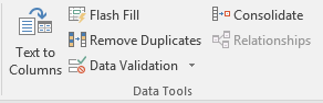
4. Remove duplicate data points or sets.

Larger data sets tend to have duplicate content. You may have a list of multiple contacts in a company and only want to see the number of companies you have. In situations like this, removing the duplicates comes in quite handy.

To remove your duplicates, highlight the row or column that you want to remove duplicates of. Then, go to the Data tab and select «Remove Duplicates» (which is under the Tools subheader in the older version of Excel). A pop-up will appear to confirm which data you want to work with. Select «Remove Duplicates,» and you’re good to go.

You can also use this feature to remove an entire row based on a duplicate column value. So if you have three rows with Harry Potter’s information and you only need to see one, then you can select the whole dataset and then remove duplicates based on email. Your resulting list will have only unique names without any duplicates.

5. Transpose rows into columns.

When you have rows of data in your spreadsheet, you might decide you actually want to transform the items in one of those rows into columns (or vice versa). It would take a lot of time to copy and paste each individual header — but what the transpose feature allows you to do is simply move your row data into columns, or the other way around.

Start by highlighting the column that you want to transpose into rows. Right-click it, and then select «Copy.» Next, select the cells on your spreadsheet where you want your first row or column to begin. Right-click on the cell, and then select «Paste Special.» A module will appear — at the bottom, you’ll see an option to transpose. Check that box and select OK. Your column will now be transferred to a row or vice-versa.

On newer versions of Excel, a drop-down will appear instead of a pop-up.

6. Split up text information between columns.

What if you want to split out information that’s in one cell into two different cells? For example, maybe you want to pull out someone’s company name through their email address. Or perhaps you want to separate someone’s full name into a first and last name for your email marketing templates.

Thanks to Excel, both are possible. First, highlight the column that you want to split up. Next, go to the Data tab and select «Text to Columns.» A module will appear with additional information.

First, you need to select either «Delimited» or «Fixed Width.»

• «Delimited» means you want to break up the column based on characters such as commas, spaces, or tabs.
• «Fixed Width» means you want to select the exact location on all the columns that you want the split to occur.

In the example case below, let’s select «Delimited» so we can separate the full name into first name and last name.

Then, it’s time to choose the Delimiters. This could be a tab, semi-colon, comma, space, or something else. («Something else» could be the «@» sign used in an email address, for example.) In our example, let’s choose the space. Excel will then show you a preview of what your new columns will look like.

When you’re happy with the preview, press «Next.» This page will allow you to select Advanced Formats if you choose to. When you’re done, click «Finish.»

7. Use formulas for simple calculations.

In addition to doing pretty complex calculations, Excel can help you do simple arithmetic like adding, subtracting, multiplying, or dividing any of your data.

• To add, use the + sign.
• To subtract, use the — sign.
• To multiply, use the * sign.
• To divide, use the / sign.

You can also use parentheses to ensure certain calculations are done first. In the example below (10+10*10), the second and third 10 were multiplied together before adding the additional 10. However, if we made it (10+10)*10, the first and second 10 would be added together first.

8. Get the average of numbers in your cells.

If you want the average of a set of numbers, you can use the formula =AVERAGE(Cell1:Cell2). If you want to sum up a column of numbers, you can use the formula =SUM(Cell1:Cell2).

9. Use conditional formatting to make cells automatically change color based on data.

Conditional formatting allows you to change a cell’s color based on the information within the cell. For example, if you want to flag certain numbers that are above average or in the top 10% of the data in your spreadsheet, you can do that. If you want to color code commonalities between different rows in Excel, you can do that. This will help you quickly see information that is important to you.

To get started, highlight the group of cells you want to use conditional formatting on. Then, choose «Conditional Formatting» from the Home menu and select your logic from the dropdown. (You can also create your own rule if you want something different.) A window will pop up that prompts you to provide more information about your formatting rule. Select «OK» when you’re done, and you should see your results automatically appear.

10. Use the IF Excel formula to automate certain Excel functions.

Sometimes, we don’t want to count the number of times a value appears. Instead, we want to input different information into a cell if there is a corresponding cell with that information.

For example, in the situation below, I want to award ten points to everyone who belongs in the Gryffindor house. Instead of manually typing in 10’s next to each Gryffindor student’s name, I can use the IF Excel formula to say that if the student is in Gryffindor, then they should get ten points.

The formula is: IF(logical_test, value_if_true, [value_if_false])

Example Shown Below: =IF(D2=»Gryffindor»,»10″,»0″)

In general terms, the formula would be IF(Logical Test, value of true, value of false). Let’s dig into each of these variables.

• Logical_Test: The logical test is the «IF» part of the statement. In this case, the logic is D2=»Gryffindor» because we want to make sure that the cell corresponding with the student says «Gryffindor.» Make sure to put Gryffindor in quotation marks here.
• Value_if_True: This is what we want the cell to show if the value is true. In this case, we want the cell to show «10» to indicate that the student was awarded the 10 points. Only use quotation marks if you want the result to be text instead of a number.
• Value_if_False: This is what we want the cell to show if the value is false. In this case, for any student not in Gryffindor, we want the cell to show «0». Only use quotation marks if you want the result to be text instead of a number.

Note: In the example above, I awarded 10 points to everyone in Gryffindor. If I later wanted to sum the total number of points, I wouldn’t be able to because the 10’s are in quotes, thus making them text and not a number that Excel can sum.

The real power of the IF function comes when you string multiple IF statements together, or nest them. This allows you to set multiple conditions, get more specific results, and ultimately organize your data into more manageable chunks.

Ranges are one way to segment your data for better analysis. For example, you can categorize data into values that are less than 10, 11 to 50, or 51 to 100. Here’s how that looks in practice: 

=IF(B3<11,“10 or less”,IF(B3<51,“11 to 50”,IF(B3<100,“51 to 100”)))

It can take some trial-and-error, but once you have the hang of it, IF formulas will become your new Excel best friend.

11. Use dollar signs to keep one cell’s formula the same regardless of where it moves.

Have you ever seen a dollar sign in an Excel formula? When used in a formula, it isn’t representing an American dollar; instead, it makes sure that the exact column and row are held the same even if you copy the same formula in adjacent rows.

You see, a cell reference — when you refer to cell A5 from cell C5, for example — is relative by default. In that case, you’re actually referring to a cell that’s five columns to the left (C minus A) and in the same row (5). This is called a relative formula. When you copy a relative formula from one cell to another, it’ll adjust the values in the formula based on where it’s moved. But sometimes, we want those values to stay the same no matter whether they’re moved around or not — and we can do that by turning the formula into an absolute formula.

To change the relative formula (=A5+C5) into an absolute formula, we’d precede the row and column values by dollar signs, like this: (=$A$5+$C$5). (Learn more on Microsoft Office’s support page here.)

12. Use the VLOOKUP function to pull data from one area of a sheet to another.

Have you ever had two sets of data on two different spreadsheets that you want to combine into a single spreadsheet?

For example, you might have a list of people’s names next to their email addresses in one spreadsheet, and a list of those same people’s email addresses next to their company names in the other — but you want the names, email addresses, and company names of those people to appear in one place.

I have to combine data sets like this a lot — and when I do, the VLOOKUP is my go-to formula.

Before you use the formula, though, be absolutely sure that you have at least one column that appears identically in both places. Scour your data sets to make sure the column of data you’re using to combine your information is exactly the same, including no extra spaces.

The formula: =VLOOKUP(lookup value, table array, column number, Approximate match (TRUE) or Exact match (FALSE))

The formula with variables from our example below: =VLOOKUP(C2,Sheet2!A:B,2,FALSE)

In this formula, there are several variables. The following is true when you want to combine information in Sheet 1 and Sheet 2 onto Sheet 1.

• Lookup Value: This is the identical value you have in both spreadsheets. Choose the first value in your first spreadsheet. In the example that follows, this means the first email address on the list, or cell 2 (C2).
• Table Array: The table array is the range of columns on Sheet 2 you’re going to pull your data from, including the column of data identical to your lookup value (in our example, email addresses) in Sheet 1 as well as the column of data you’re trying to copy to Sheet 1. In our example, this is «Sheet2!A:B.» «A» means Column A in Sheet 2, which is the column in Sheet 2 where the data identical to our lookup value (email) in Sheet 1 is listed. The «B» means Column B, which contains the information that’s only available in Sheet 2 that you want to translate to Sheet 1.
• Column Number: This tells Excel which column the new data you want to copy to Sheet 1 is located in. In our example, this would be the column that «House» is located in. «House» is the second column in our range of columns (table array), so our column number is 2. [Note: Your range can be more than two columns. For example, if there are three columns on Sheet 2 — Email, Age, and House — and you still want to bring House onto Sheet 1, you can still use a VLOOKUP. You just need to change the «2» to a «3» so it pulls back the value in the third column: =VLOOKUP(C2:Sheet2!A:C,3,false).]
• Approximate Match (TRUE) or Exact Match (FALSE): Use FALSE to ensure you pull in only exact value matches. If you use TRUE, the function will pull in approximate matches.

In the example below, Sheet 1 and Sheet 2 contain lists describing different information about the same people, and the common thread between the two is their email addresses. Let’s say we want to combine both datasets so that all the house information from Sheet 2 translates over to Sheet 1.

So when we type in the formula =VLOOKUP(C2,Sheet2!A:B,2,FALSE), we bring all the house data into Sheet 1.

Keep in mind that VLOOKUP will only pull back values from the second sheet that are to the right of the column containing your identical data. This can lead to some limitations, which is why some people prefer to use the INDEX and MATCH functions instead.

13. Use INDEX and MATCH formulas to pull data from horizontal columns.

Like VLOOKUP, the INDEX and MATCH functions pull in data from another dataset into one central location. Here are the main differences:

• VLOOKUP is a much simpler formula. If you’re working with large data sets that would require thousands of lookups, using the INDEX and MATCH function will significantly decrease load time in Excel.
• The INDEX and MATCH formulas work right-to-left, whereas VLOOKUP formulas only work as a left-to-right lookup. In other words, if you need to do a lookup that has a lookup column to the right of the results column, then you’d have to rearrange those columns in order to do a VLOOKUP. This can be tedious with large datasets and/or lead to errors.

So if I want to combine information in Sheet 1 and Sheet 2 onto Sheet 1, but the column values in Sheets 1 and 2 aren’t the same, then to do a VLOOKUP, I would need to switch around my columns. In this case, I’d choose to do an INDEX and MATCH instead.

Let’s look at an example. Let’s say Sheet 1 contains a list of people’s names and their Hogwarts email addresses, and Sheet 2 contains a list of people’s email addresses and the Patronus that each student has. (For the non-Harry Potter fans out there, every witch or wizard has an animal guardian called a «Patronus» associated with him or her.) The information that lives in both sheets is the column containing email addresses, but this email address column is in different column numbers on each sheet. I’d use the INDEX and MATCH formulas instead of VLOOKUP so I wouldn’t have to switch any columns around.

So what’s the formula, then? The formula is actually the MATCH formula nested inside the INDEX formula. You’ll see I differentiated the MATCH formula using a different color here.

The formula: =INDEX(table array, MATCH formula)

This becomes: =INDEX(table array, MATCH (lookup_value, lookup_array))

The formula with variables from our example below: =INDEX(Sheet2!A:A,(MATCH(Sheet1!C:C,Sheet2!C:C,0)))

Here are the variables:

• Table Array: The range of columns on Sheet 2 containing the new data you want to bring over to Sheet 1. In our example, «A» means Column A, which contains the «Patronus» information for each person.
• Lookup Value: This is the column in Sheet 1 that contains identical values in both spreadsheets. In the example that follows, this means the «email» column on Sheet 1, which is Column C. So: Sheet1!C:C.
• Lookup Array: This is the column in Sheet 2 that contains identical values in both spreadsheets. In the example that follows, this refers to the «email» column on Sheet 2, which happens to also be Column C. So: Sheet2!C:C.

Once you have your variables straight, type in the INDEX and MATCH formulas in the top-most cell of the blank Patronus column on Sheet 1, where you want the combined information to live.

14. Use the COUNTIF function to make Excel count words or numbers in any range of cells.

Instead of manually counting how often a certain value or number appears, let Excel do the work for you. With the COUNTIF function, Excel can count the number of times a word or number appears in any range of cells.

For example, let’s say I want to count the number of times the word «Gryffindor» appears in my data set.

The formula: =COUNTIF(range, criteria)

The formula with variables from our example below: =COUNTIF(D:D,»Gryffindor»)

In this formula, there are several variables:

• Range: The range that we want the formula to cover. In this case, since we’re only focusing on one column, we use «D:D» to indicate that the first and last column are both D. If I were looking at columns C and D, I would use «C:D.»
• Criteria: Whatever number or piece of text you want Excel to count. Only use quotation marks if you want the result to be text instead of a number. In our example, the criteria is «Gryffindor.»

Simply typing in the COUNTIF formula in any cell and pressing «Enter» will show me how many times the word «Gryffindor» appears in the dataset.

15. Combine cells using &.

Databases tend to split out data to make it as exact as possible. For example, instead of having a column that shows a person’s full name, a database might have the data as a first name and then a last name in separate columns. Or, it may have a person’s location separated by city, state, and zip code. In Excel, you can combine cells with different data into one cell by using the «&» sign in your function.

The formula with variables from our example below: =A2&» «&B2

Let’s go through the formula together using an example. Pretend we want to combine first names and last names into full names in a single column. To do this, we’d first put our cursor in the blank cell where we want the full name to appear. Next, we’d highlight one cell that contains a first name, type in an «&» sign, and then highlight a cell with the corresponding last name.

But you’re not finished — if all you type in is =A2&B2, then there will not be a space between the person’s first name and last name. To add that necessary space, use the function =A2&» «&B2. The quotation marks around the space tell Excel to put a space in between the first and last name.

To make this true for multiple rows, simply drag the corner of that first cell downward as shown in the example.

16. Add checkboxes.

If you’re using an Excel sheet to track customer data and want to oversee something that isn’t quantifiable, you could insert checkboxes into a column.

For example, if you’re using an Excel sheet to manage your sales prospects and want to track whether you called them in the last quarter, you could have a «Called this quarter?» column and check off the cells in it when you’ve called the respective client.

Here’s how to do it.

Highlight a cell you’d like to add checkboxes to in your spreadsheet. Then, click DEVELOPER. Then, under FORM CONTROLS, click the checkbox or the selection circle highlighted in the image below.

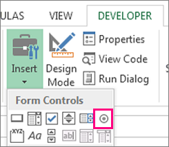
Once the box appears in the cell, copy it, highlight the cells you also want it to appear in, and then paste it.

17. Hyperlink a cell to a website.

If you’re using your sheet to track social media or website metrics, it can be helpful to have a reference column with the links each row is tracking. If you add a URL directly into Excel, it should automatically be clickable. But, if you have to hyperlink words, such as a page title or the headline of a post you’re tracking, here’s how.

Highlight the words you want to hyperlink, then press Shift K. From there a box will pop up allowing you to place the hyperlink URL. Copy and paste the URL into this box and hit or click Enter.

If the key shortcut isn’t working for any reason, you can also do this manually by highlighting the cell and clicking Insert > Hyperlink.

18. Add drop-down menus.

Sometimes, you’ll be using your spreadsheet to track processes or other qualitative things. Rather than writing words into your sheet repetitively, such as «Yes», «No», «Customer Stage», «Sales Lead», or «Prospect», you can use dropdown menus to quickly mark descriptive things about your contacts or whatever you’re tracking.

Here’s how to add drop-downs to your cells.

Highlight the cells you want the drop-downs to be in, then click the Data menu in the top navigation and press Validation.

From there, you’ll see a Data Validation Settings box open. Look at the Allow options, then click Lists and select Drop-down List. Check the In-Cell dropdown button, then press OK.

19. Use the format painter. 

As you’ve probably noticed, Excel has a lot of features to make crunching numbers and analyzing your data quick and easy. But if you ever spent some time formatting a sheet to your liking, you know it can get a bit tedious.

Don’t waste time repeating the same formatting commands over and over again. Use the format painter to easily copy the formatting from one area of the worksheet to another. To do so, choose the cell you’d like to replicate, then select the format painter option (paintbrush icon) from the top toolbar.

Excel Keyboard Shortcuts 

Creating reports in Excel is time-consuming enough. How can we spend less time navigating, formatting, and selecting items in our spreadsheet? Glad you asked. There are a ton of Excel shortcuts out there, including some of our favorites listed below.

Create a New Workbook

PC: Ctrl-N | Mac: Command-N

Select Entire Row

PC: Shift-Space | Mac: Shift-Space

Select Entire Column

PC: Ctrl-Space | Mac: Control-Space

Select Rest of Column

PC: Ctrl-Shift-Down/Up | Mac: Command-Shift-Down/Up

Select Rest of Row

PC: Ctrl-Shift-Right/Left | Mac: Command-Shift-Right/Left

Add Hyperlink

PC: Ctrl-K | Mac: Command-K

Open Format Cells Window

PC: Ctrl-1 | Mac: Command-1

Autosum Selected Cells

PC: Alt-= | Mac: Command-Shift-T

Other Excel Help Resources

• How to Make a Chart or Graph in Excel [With Video Tutorial]
• Design Tips to Create Beautiful Excel Charts and Graphs
• Totally Free Microsoft Excel Templates That Make Marketing Easier
• How to Learn Excel Online: Free and Paid Resources for Excel Training

Use Excel to Automate Processes in Your Team

Even if you’re not an accountant, you can still use Excel to automate tasks and processes in your team. With the tips and tricks we shared in this post, you’ll be sure to use Excel to its fullest extent and get the most out of the software to grow your business.

Editor’s Note: This post was originally published in August 2017 but has been updated for comprehensiveness.

17th January 2019

Progression. It’s something we all get our knickers in a twist about. Either it’s not happening fast enough, or it’s not in the area we want or it’s just simply not happening altogether. Whether it’s in your career, your personal life, your side hustle whatev. There are 4 surefire ways to progress in whatever it is you want:

Be engaged and enthusiastic

If you want to excel you need to be engaged in what you’re doing. Bit of a given huh? But one that seems to be completely forgotten about when people moan they’re not progressing fast enough. You have to put the effort in. I’m not saying that you cut out sleep on a Wednesday and Saturday and have a to-do list the length of the garden. (although being organised is never a bad thing). But having passion in what you’re doing and being consistent is the key to anything and everything.

Story time: there’s someone in my office who within the first week in their role, would sit thumbing through Tinder whilst someone was trying to train them 1-on-1. Who are these people? The audacity, I can’t. Deceased.

Always put your hand up

This is something I’m personally striving to get better at. Getting out of my comfort zone and take every opportunity I’m faced with. Whether it’s training, a new skill, anything. Putting yourself out there, and adding another string to your bow will only ever benefit you. If nothing else you will gain experience, you’ll learn a little something about yourself and your abilities. You may even surprise yourself.

Go for that promotion, put your name down for training on a subject you’re uncomfortable with, accept that email that pushes you. It’ll help you grow and give you the confidence to take the next step.

Start schmoozing

The oldest cliche there is, ‘it’s not what you know, it’s who you know’, and it’s true. Think about it, if you’re recruiting for a role/campaign/promotion (whatev) you’re more than likely going to look favourably at someone you have an existing relationship with. You already know what they’re like, how they operated, the quality of their work and to be honest, it’s just so much bloody easier.

Try and get your name out there in a positive way, and remember that ‘they’re just people’. Regardless of anyone’s title or status, they’re still a person. They eat and shower and pick their nose, just like you.

Showcase your passions

Any chance you get, whatever your passion maybe, showcase it. I work in insurance, my passion (surprisingly) isn’t insurance, however I love being creative and writing. And so I write the online posts for our building, I helped organise our biggest event of the year, and now I’m known for that. I showed my skills and I’m the go-to. Show them what you can do, trust me if your passion shines through, no one will forget you.

outfit deats
giraffe print blouse – River Island, £28.00

Yes, You have to excel in everything you do. Not because you have a passion on it but because you have to do it in order to activate your full potential or hidden talent. Sometimes we need to push our self

Author: appleblog18

I guess I’m just an open-hearted, fair, good person. I try to encourage people to be their best and look inside themselves and find out what they are passionate about and expand on that and enjoy life.
View all posts by appleblog18

Leave a Reply

Enter your comment here…

Fill in your details below or click an icon to log in:

Email (required) (Address never made public)

Name (required)

Website

You are commenting using your WordPress.com account.
( Log Out / 
Change )

You are commenting using your Twitter account.
( Log Out / 
Change )

You are commenting using your Facebook account.
( Log Out / 
Change )

Cancel

Connecting to %s

Notify me of new comments via email.

Notify me of new posts via email.

Work in Excel for the web

Name your file

When you create a workbook, Excel for the web automatically names it. To change the name:

1. Select the name.

2. Type a meaningful name and then press Enter.

   Everything you do in Excel for the web — naming a file, entering data — is automatically saved to your OneDrive.

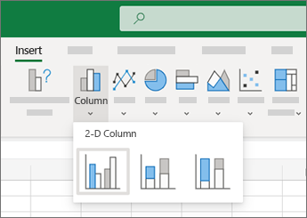
Do your work

After you name your file, you can enter data and create tables, charts, and formulas. Select the tabs at the top to find the features you want.

To collapse the ribbon and make more space, select the down arrow  on the far right. 

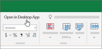
Need the full set of Excel features?

Open your file in the Excel desktop app one of two ways, depending on what you see in your workbook:

• Select Open in Desktop App at the top of your workbook. If you don’t see it, there should be a search bar along the top of your workbook. In that search bar, type open, and then select Open in Desktop App.

The Excel app will launch and open the file. Continue working and save.

When you save changes in the desktop app, they save to OneDrive — no need to Save As and re-upload the file.

На основании Вашего запроса эти примеры могут содержать грубую лексику.

На основании Вашего запроса эти примеры могут содержать разговорную лексику.

They can juggle a whole lot of activities and yet excel in everything they undertake.

Pisces say, ‘do your best’ while Geminis excel in everything they do naturally.

Рыбы говорят: «делайте все возможное», в то время как Близнецы достигают всего естественным образом.

They’re the «good» daughters and sons who do what they’re told, try to excel in everything they do, and focus on pleasing others.

Это «хорошие» дочери и сыновья, которые делают то, что им говорят, стараются преуспеть во всем, что делают, и сосредоточены на том, чтобы радовать других.

We cannot be experts in everything and excel in everything.

Ничего не найдено для этого значения.

Результатов: 16559. Точных совпадений: 3. Затраченное время: 278 мс

Documents

Корпоративные решения

Спряжение

Синонимы

Корректор

Справка и о нас

Индекс слова: 1-300, 301-600, 601-900

Индекс выражения: 1-400, 401-800, 801-1200

Индекс фразы: 1-400, 401-800, 801-1200

How To Use Excel: A Beginner’s Guide To Getting Started

How To Use Excel:
A Beginner’s Guide To Getting Started

Written by co-founder Kasper Langmann, Microsoft Office Specialist.

Excel is a powerful application—but it can also be very intimidating.

That’s why we’ve put together this beginner’s guide to getting started with Excel.

It will take you from the very beginning (opening a spreadsheet), through entering and working with data, and finish with saving and sharing.

It’s everything you need to know to get started with Excel.

If you want to tag along as you read, please download the free sample Excel workbook here.

Opening an Excel spreadsheet

When you first open Excel (by double-clicking the icon or selecting it from the Start menu), the application will ask what you want to do.

If you want to open a new Excel spreadsheet, click Blank workbook.

To open an existing spreadsheet (like the example workbook you just downloaded), click Open Other Workbooks in the lower-left corner, then click Browse on the left side of the resulting window.

Then use the file explorer to find the Excel workbook you’re looking for, select it, and click Open.

Workbooks vs. spreadsheets

There’s something we should clear up before we move on.

A workbook is an Excel file. It usually has a file extension of .XLSX (if you’re using an older version of Excel, it could be .XLS).

A spreadsheet is a single sheet inside a workbook. There can be many sheets inside of a workbook, and they’re accessed via the tabs at the bottom of the screen.

A spreadsheet (a.k.a. a sheet/tab) contains all the cells you can see and use in the >1 million rows >16,000 columns.

Working with the Ribbon

The Ribbon is the central control panel of Excel. You can do just about everything you need to directly from the Ribbon.

Where is this powerful tool? At the top of the window:

There are a number of tabs, including the File tab, Home tab, Insert tab, Data tab, Review tab, and a few others. Each tab contains different buttons.

Try clicking on a few different tabs to see which buttons appear below them.

Kasper Langmann, Co-founder of Spreadsheeto

There’s also a very useful search bar in the Ribbon. It says Tell me what you want to do. Just type in what you’re looking for, and Excel will help you find it.

Most of the time, you’ll be in the Home tab of the Ribbon. But Formulas and Data are also very useful (we’ll be talking about formulas shortly).

Pro tip: Ribbon sections

In addition to tabs, the Ribbon also has some smaller sections. And when you’re looking for something specific, those sections can help you find it.

For example, if you’re looking for sorting and filtering options, you don’t want to hover over dozens of buttons finding out what they do.

Instead, skim through the section names until you find what you’re looking for:

Managing your sheets

As we saw, workbooks can contain multiple sheets.

You can manage those sheets with the sheet tabs near the bottom of the screen. Click a tab to open that particular worksheet.

If you’re using our example workbook, you’ll see two sheets, called Welcome and Thank You:

To add a new worksheet, click the + (plus) button at the end of the list of sheets.

You can also reorder the sheets in your workbook by dragging them to a new location.

And if you right-click a worksheet tab, you’ll get a number of options:

For now, don’t worry too much about these options. Rename and Delete are useful, but the rest needn’t concern you.

Kasper Langmann, Co-founder of Spreadsheeto

Entering data

Now it’s time to enter some data!

And while entering data is one of the most central and important things you can do in Excel, it’s almost effortless.

Just click into a blank cell and start typing.

Go ahead, try it! Type your name, birthday, and your favorite number into some blank cells.

Kasper Langmann, Co-founder of Spreadsheeto

You can also copy (Ctrl + C), cut (Ctrl + X), and paste (Ctrl + V) any data you’d like (or read our full guide on copying and pasting here).

Try copying and pasting the data from multiple cells inthe example spreadsheet into another column.

You can also copy data from other programs into Excel.

Try copying this list of numbers and pasting it into your sheet:

• 17
• 24
• 9
• 00
• 3
• 12

That’s all we’re going to cover for basic data entry. Just know that there are lots of other ways to get data into your spreadsheets if you need them.

Kasper Langmann, Co-founder of Spreadsheeto

Basic calculations

Now that we’ve seen how to get some basic data into our spreadsheet, we’re going to do some things with it.

Running basic calculations in Excel is easy. First, we’ll look at how to add two numbers.

Important: start calculations with = (equals)

When you’re running a calculation (or a formula, which we’ll discuss next), the first thing you need to type is an equals sign. This tells Excel to get ready to run some sort of calculation.

So when you see something like =MEDIAN(A2:A51), make sure you type it exactly as it is—including the equals sign.

Let’s add 3 and 4. Type the following formula in a blank cell:

=3+4

Then hit Enter.

When you hit Enter, Excel evaluates your equation and displays the result, 7.

But if you look above at the formula bar, you’ll still see the original formula.

That’s a useful thing to keep in mind, in case you forget what you typed originally.

You can also edit a cell in the formula bar. Click on any cell, then click into the formula bar and start typing.

Kasper Langmann, Co-founder of Spreadsheeto

Performing subtraction, multiplication, and division is just as easy. Try these formulas:

• =4-6
• =2*5
• =-10/3

What we’re going to cover next is one of the most important things in Excel. We’re giving it a very basic overview here, but feel free to read our post on cell references to get the details.

Kasper Langmann, Co-founder of Spreadsheeto

Now let’s try something different. Open up the first sheet in the example workbook, click into cell C1, and type the following:

=A1+B1

Hit Enter.

You should get 82, the sum of the numbers in cells A1 and B1.

Now, change one of the numbers in A1 or B1 and watch what happens:

Because you’re adding A1 and B1, Excel automatically updates the total when you change the values in one of those cells.

Try doing different types of arithmetic on the other numbers in columns A and B using this method.

Unlocking the power of functions

Excel’s greatest power lies in functions. These let you run complex calculations with a few keypresses.

We’ll barely scratch the surface of functions here. Check out our other blog posts to see some of the great things you can do with functions!

Kasper Langmann, Co-founder of Spreadsheeto

Many formulas take sets of numbers and give you information about them.

For example, the AVERAGE function gives you the average of a set of numbers. Let’s try using it.

Click into an empty cell and type the following formula:

=AVERAGE(A1:A4)

Then hit Enter.

The resulting number, 0.25, is the average of the numbers in cells A1, A2, A3, and A4.

Cell range notation

In the formula above, we used “A1:A4” to tell Excel to look at all the cells between A1 and A4, including both of those cells. You can read it as “A1 through A4.”

You can also use this to include numbers in different columns. “A5:C7” includes A5, A6, A7, B5, B6, B7, C5, C6, and C7.

There are also functions that work on text.

Let’s try the CONCATENATE function!

Click into cell C5 and type this formula:

=CONCATENATE(A5, ” “, B5)

Then hit Enter.

You’ll see the message “Welcome to Spreadsheeto” in the cell.

How did this happen? CONCATENATE takes cells with text in them and puts them together.

We put the contents of A5 and B5 together. But because we also needed a space between “to” and “Spreadsheeto,” we included a third argument: the space between two quotes.

Remember that you can mix cell references (like “A5″) and typed values (like ” “) in formulas.

Kasper Langmann, Co-founder of Spreadsheeto

Excel has dozens of useful functions. To find the function that will solve a particular problem, head to the Formulas tab and click on one of the icons:

Scroll through the list of available functions, and select the one you want (you may have to look around for a while).

Then Excel will help you get the right numbers in the right places:

If you start typing a formula, starting with the equals sign, Excel will help you by showing you some possible functions that you might be looking for:

And finally, once you’ve typed the name of a formula and the opening parenthesis, Excel will tell you which arguments need to go where:

If you’ve never used a function before, it might be difficult to interpret Excel’s reminders. But once you get more experience, it’ll become clear.

This is a tiny preview of how functions work and what they can do. It should be enough to get you going on the tasks you need to accomplish right away.

Kasper Langmann, Co-founder of Spreadsheeto

Saving and sharing your work

After you’ve done a bunch of work with your spreadsheet, you’re going to want to save your changes.

Hit Ctrl + S to save. If you haven’t yet saved your spreadsheet, you’ll be asked where you want to save it and what you want to call it.

You can also click the Save button in the Quick Access Toolbar:

It’s a good idea to get into the habit of saving often. Trying to recover unsaved changes is a pain!

Kasper Langmann, Co-founder of Spreadsheeto

The easiest way to share your spreadsheets is via OneDrive.

Click the Share button in the top-right corner of the window, and Excel will walk you through sharing your document.

You can also save your document and email it, or use any other cloud service to share it with others.

That’s it – Now what?

This was how to use Excel.

Or… at least a small fraction of it.

Microsoft Excel can be intimidating, but once you get the basics down, it’s easier to learn the more advanced functions.

This was your introduction to “the basics”. So, if you’re not ready to get some advanced Excel knowledge, go ahead and practice with some of the existing data at the office 🧑🏼‍💻

If you’re ready to take your next steps, go ahead and enroll in my 30-minute free online course where you learn: IF, SUMIF, VLOOKUP, and data cleaning.

These are some of the most important topics of Excel💪🏼

Other resources

Now, you can’t excel at Excel without mastering some of the lookup functions like VLOOKUP and the new XLOOKUP.

But also, you don’t wanna miss out on pivot tables. You can use these to transform your Microsoft Excel data into insightful reports in just a few clicks🤯

Or if you’re into automating Excel spreadsheet formatting, go ahead and read my guide to conditional formatting here.

Kasper Langmann2023-02-23T14:45:07+00:00

When it comes to Excel, there isn’t much middle ground.

You have people who absolutely love it and will sing the praises of spreadsheets all day. And, then you have the people who absolutely detest it. They’d rather lock themselves in a phone booth full of mosquitos than have to go cross-eyed looking at all of those columns and rows.

Admittedly, I used to fall into that latter group. I’d open a new Excel workbook with the best of intentions. But, after 20 odd minutes of trying to get one stupid decimal point to appear properly in its cell, I’d throw my hands up once again and claim Excel just wasn’t for me.

Then, my life experienced a major plot twist: I married a total Excel whiz—someone who literally spends his entire workday creating complicated macros and some of the most impressive spreadsheets I’ve ever seen. And, he’s made it his personal mission to convert me to his tribe of Excel-lovers (honestly, I’m surprised it wasn’t in his wedding vows).

Since then? Well, he’s made some progress. I’ve been able to put my hatred aside and recognize that learning Excel can actually be an incredibly powerful tool for combing through information and finding exactly what you need—provided you know how to use it correctly.

It’s that last part that trips people up. But, fortunately, Excel isn’t nearly as complicated as you’re likely making it out to be.

In fact, there are plenty of helpful tricks and tools you can utilize—whether you’re a total newbie or an established expert. Here are six things you should absolutely know how to do in Excel (and, trust me, you’ll be glad you do!).

---

---

1. Sort data

Typically, spreadsheets are useful for storing and sorting a whole bunch of information—think a contact list for 800 people that you want to invite to your company’s luncheon, for example.

Now, let’s say that you want to sort those people accordingly. Perhaps you want them listed in alphabetical order by last name. Or, maybe you want to group them together by city.

Excel makes it easy to comb through your entire data set and sort everything into a clean and easy to read spreadsheet.

Here’s how you do it:

• Highlight the entire data set you want to sort (not just one column!) by either dragging your cursor across all of the cells or clicking the triangle in the upper left of your spreadsheet to select the entire thing.
• Hit the “Data” tab.
• Click the “Sort” button.
• Select how you want to sort your data (in the example below, I sorted by city!).
• Hit “OK.”

Then, your data will be sorted accordingly—in this case, alphabetical order by city.

IMPORTANT NOTE: It’s important that you select the entire data set you want to sort, and not just one column. That way, your rows will stay intact—meaning, in this case, the correct address will stay with the appropriate person.

Had I just selected the first column, Excel would’ve sorted only that one column alphabetically, making the addresses a mismatched mess.

2. Remove duplicates

It’s inevitable: When you’re working with a large dataset, there are bound to be a few duplicates that sneak their way in.

Rather than getting bleary-eyed and frustrated by scrolling through that entire spreadsheet and looking for them yourself, Excel can do all of that legwork for you and remove duplicates with the click of a button.

Here’s how you do it:

• Highlight the entire data set.
• Hit the “Data” tab.
• Click the “Remove Duplicates” button.
• Select what columns you want Excel to find duplicates in.
• Hit “OK.”

IMPORTANT NOTE: Be careful that you choose enough qualifiers to weed out the true duplicates. For example, if I had just selected to remove duplicates in only Column A above (meaning Excel would’ve looked for duplicates of “Oprah”), I would’ve deleted one Oprah that indeed had the same address, but one that had a different last name and address altogether (a different Oprah entirely!)

The bottom line is, utilize enough information so that you’re removing rows that are true identical copies of each other—and don’t just share one similar value!

---

---

3. Basic math functions

Stop reaching for that calculator—Excel can handle all sorts of math functions for you! All you need to do is enter a few simple formulas.

Think that sounds like it’s way beyond your Excel knowledge? Think again. Trust me, if I can figure this out, so you can you.

Here are the basic formulas you’ll want to know:

• Addition: Type “=SUM” in a blank cell where you want the total to appear, click the cells you want to add together, and then hit “Enter.”
• Subtraction: Type “=” in a blank cell where you want the difference to appear, click the cell you want to subtract from, type “-”, click the cell you want to subtract, and then hit enter.
• Multiplication: Type “=” in a blank cell where you want the total to appear, click the cell for a number you want to multiply, type “*”, click the cell for the other number you want to multiply, and then hit enter.
• Division: Type “=” in a blank cell where you want the remainder to appear, click the cell for the number you want to divide, type “/”, click the cell for the number you want to divide by, and then hit enter.

Listen, I know these are a little confusing to put down in words. But, give them a try for yourself and I’m positive you’ll quickly see that they aren’t complicated at all. Here’s a look at what the SUM function looks like in practice:

INSIDER TIP: If you want to drag the same mathematical formula across a row, you can! After entering the formula into one cell, click that cell where the total appeared, click the little green box that appears in the lower right-hand corner, and drag it across the rest of the row where you need that formula to be applied.

Voila—it’ll happen automatically! You’ll be able to crunch numbers in different columns, without needing to enter the formula again and again.

4. Freeze panes

There’s nothing worse than scrolling through a huge spreadsheet that requires you to continuously go back up to the top to see what your column headers are.

Fortunately, you can make your column headers and your row numbers stay right where they are—meaning you can always see them, no matter how far down the spreadsheet you go. You can do this by using Excel’s handy “freeze panes” feature.

Here’s how you do it:

• Click on the row underneath your column headers.
• Click on the “View” tab.
• Click the “Freeze Panes” button.

Scroll down and across your spreadsheet, and you’ll see that the information you need is always right there within view!

5. Insert current date

Sick of glancing at your calendar or the bottom of your computer monitor in order to get today’s date and enter it in your spreadsheet?

Excel can do it for you—with just one easy keyboard shortcut. Here it is:

Ctrl + ;

Put your cursor in the cell where you want the date to appear, use that shortcut, and Excel will automatically fill in today’s date for you. Easy peasy!

IMPORTANT NOTE: Dates entered using that function are static, meaning they won’t change as your spreadsheet ages!

6. Make the same change across worksheets

When you’re working with multiple tabs, it’s a hassle to comb through them all and make the same change over and over again. Fortunately, you don’t have to!

You can select the appropriate sheets in your workbook where that change should appear. Make the change once, and it’ll be applied across all of the sheets you selected.

Here’s how you do it:

• Hold the “Command” key on your keyboard (or “Control” if you’re using a PC).
• Select the appropriate tabs of your workbook.
• Make the necessary change to one cell.
• Check to make sure it applied across all of your worksheets.

Want to see this in practice? For simplicity’s sake, let’s assume I got married to Aaron Rodgers (hey, a girl can dream!). As a result, I changed my last name from “Boogaard” to “Rodgers.” Since my name appears in numerous different tabs of this spreadsheet, I’d use this handy trick to only have to enter my new last name one time.

And that’s what you need to know how to do in Excel

I get it—Excel can feel a little intimidating. But, once you start playing around, you’ll begin to become more and more comfortable and quickly begin to realize just how much easier it can make things for you.

Get your start by mastering these six basic Excel tricks, and you’ll be on the path to becoming a total Excel whiz in no time!

Excel may seem like a basic spreadsheet tool, but it has many use cases. Here are some of the practical uses of Excel in daily life.

Excel has long been considered the best tool for data analysts. But Excel’s uses are not restricted to people who work on data regularly. As a layman, there are plenty of Excel uses, which can ease your day-to-day work responsibilities. You can do everything from maintaining attendance in an office/school to creating elaborate budgets to manage your monthly expenditures in Excel.

Excel’s flexibility, multi-faceted usage, and easy-to-use functions make it one of the most preferred applications. If you’re a regular Excel user, here are a few ways to use the application in some related fields.

1. Information Management

Excel has widespread uses in a business environment, especially when managing common frameworks. From using it to drive sales reporting to preparing inventory trackers, there is a bit of everything in Excel. Here are some things you can use Excel within the information management domain:

1. Sales Inventory Tracker: Excel has proved its worth within the supply chain management sector. Since it can hold multiple rows of data, it’s a preferred choice for businesses and organizations dealing with products and services. Whenever you are tracking inventory, you can create plenty of pivots and functions to keep track of the various product levels. This way, you can never go wrong with your inventory management and stay on top of your orders and reorders. For best results, you can create an automated data entry form in Excel to ease your data management woes.
2. Attendance Trackers: As an employee-centric company, you can use Excel to track your employees’ reporting time, manage their attendance, and create elaborate dashboards to follow their regular work schedules. Each element ties into a more extensive dashboard, wherein you can get a consolidated snapshot of your employees’ whereabouts.
3. Performance Reporting: Imagine you need to calculate your employees’ performance metrics and key person indicators (KPIs) monthly. Excel offers everything from managing essential records to having everything in one go. Work with elaborate dashboards, apply various formulas and use their multi-faceted VBA functions to automate your regular jobs.

2. Time Management

Did you know you can use Excel sheets to create your productivity and time trackers? Yes, you read that right; Excel has a vast untapped potential to use its time-driven functions to perform various date- and time-driven specifics. Some common uses of Excel for time management include:

• Daily Planners
• Project ROTAs
• Roadmap Trackers for managing process training timelines

The list is not exhaustive; there are plenty of other ways to use Excel for time management. To take things up a notch, you can even create a Pomodoro Tracker in Excel to stay focused on your tasks.

3. Goal Planning & Tracking Progress

Goal planning is an essential task in every project management field. For example, you can create elaborate time-tracking tools like Gantt charts and other task-driven goal sheets to drive productivity within Excel.

By creating and defining milestones, you can track progress against your goals and map the progress against each aspect with relative ease. You can automate some tasks to track your progress as other collaborators add their progress to a common workbook.

4. Budget Management & Finance Tracking

Excel is every accountant’s friend; when you have to create detailed monthly spending trackers for your organization, you can use various in-built accounting and math-related functions to keep track of your finances, budgets, and accounts. Organizations and enterprises of various shapes, sizes, and forms use Excel in conjunction with other accounting and finance tools to enhance their accounting standards.

You can create detailed accounting and finance-related tasks to enhance your reporting. In fact, with pivots, conditional formatting, and formulas, you can create in-built alerts within Excel to highlight important aspects relevant to your business.

5. Data Analysis

Data analysis is an integral part of every organization, and many data analysts continue to favor Excel for performing data-driven tasks. You can do everything from creating elaborate performance reporting to analysis-driven hypothesis calculations in Excel. Excel’s functionality and versatility with other data analysis systems and tools have taken precedence over every other tracking system on the market.

It integrates with multiple software, and you can store endless rows of data within sheets. You can combine multiple Excel workbooks with Python and other programming languages, without lifting a finger.

6. Data Visualization

Businesses and enterprises rely on data to fuel their insights. These insights are helpful when you have to make well-informed decisions to predict the future.

What’s the best way to derive insights? It’s simple; you visualize data, so people can quickly understand what you’re trying to tell them. Create multiple graphs, or load these data sheets into visualization software like Tableau and PowerBI to bring your data to life.

Excel’s versatility comes to the fore, since you can create elaborate graphs and visualizations within the application without venturing over to other platforms. Nonetheless, it’s good to know that external integration options are available if you ever need to go down that route.

7. Expense Management

Homemakers and householders use Excel to keep track of their daily expenditures. Imagine having a simple sheet that houses all your monthly income and every possible minute expenditure, from the big spending to the small expenses.

Add formulas to auto-calculate your residual income and spending prowess for the month. While you don’t need to create elaborate accounting trackers for yourself, you can always work with simple trackers to manage your income and monthly expenditures. If you are a fan of paper-based expense trackers, you can even use free printable expense trackers to help you stay on budget.

8. Quick Calculations

Excel has become a go-to tool for people who want to perform different calculations. Imagine you wanted to calculate your next mortgage installment, but instead of using a pen and paper to make the calculations, you could quickly create an Excel workbook and start making estimates.

Excel, as an application, is handy and quite useful for performing quick calculations since it has a variety of functional formulas to help you get going.

Use of Excel in Daily Life

Excel is a wondrous language, and you can make the most of it, especially if you master the various functionalities, formulas, and procedures. However, to ensure you are using it correctly, you need to learn it from the experts. Plenty of free and paid courses are available on some famous platforms, including Udemy and a few other platforms. You can pick and choose a course that matches your learning requirements.

In this post, we’re going to learn everything there is to know about Excel Tables!

Yes, I mean everything and there’s a lot.

This post will tell you about all the awesome features Excel Tables have and why you should start using them.

What is an Excel Table?

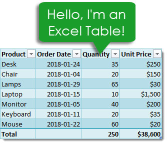
Excel Tables are containers for your data.

Imagine a house without any closets or cupboards to store your things, it would be chaos! Excel tables are like closets and cupboards for your data, they help to contain and organize data in your spreadsheets.

In your house, you might put all your plates into one kitchen cupboard. Similarly, you might put all your customer data into one Excel table.

Tables tell excel that all the data is related. Without a table, the only thing relating the data is proximity to each other.

Ok, so what’s so great about Excel Tables other than being a container to organize data? A lot actually. This post will tell you about all the awesome features tables have and should convince you to start using them.

Video Tutorial

The Parts of a Table

Throughout this post, I’ll be referring to various parts of a table, so it’s probably a good idea that we’re both talking about the same thing.

This is the Column Header Row. It is the first row in a table and contains the column headings that identify each column of data. Column headings must be unique in the table, they cannot be blank and they cannot contain formulas.

This is the Body of the table. The body is where all the data and formulas live.

This is a Row in the table. The body of a table can contain one or more rows and if you try to delete all the rows in a table a single blank row will remain.

This is a Column in the table. A table must contain at least one column.

This is the Total Row of the table. By default, tables don’t include a total row but this feature can be enabled if desired. If it’s enabled, it will be the last row of the table. This row can contain text, formula or remain blank. Each cell in the total row will have a drop down menu that allows selection of various summary formula.

Create a Table from the Ribbon

Creating an Excel Table is really easy. Select any cell inside your data and Excel will guess the range of your data when creating the table. You’ll be able to confirm this range later on. Instead of letting Excel guess the range you can also select the entire range of data in this step.

With the active cell inside your data range, go to the Insert tab in the ribbon and press the Table button found in the Tables section.

The Create Table dialog box will pop up. Excel guesses the range and you can adjust this range if needed using the range selector icon on the right hand side of the Where is the data for your table? input field. You can also adjust this range by manually typing over the range in the input field.

Checking the My table has headers box will tell Excel the first row of data contains the column headers in your table. If this is unchecked Excel will create generic column headers for the table labelled Column 1, Column 2 etc…

Press the Ok button when you’re satisfied with the data range and table headers check box.

Congratulations! You now have an Excel table and your data should look something like the above depending on the default style of your tables.

Contextual Table Tools Design Tab

Whenever you select a cell inside a table, you will notice a new tab appear in the ribbon labelled Table Tools Design. This is a contextual tab and only appears when a table is selected. When the active cell moves outside the table, the tab will disappear again.

This is where all the commands and options related to tables will live. This is where you’ll be able to name your table, find table related tools, enable or disable table elements and change your table’s style.

Create a Table with a Keyboard Shortcut

You can also create a table using a keyboard shortcut. The process is the same as described above but instead of using the Table button in the ribbon you can press Ctrl + T on your keyboard. It’s easy to remember since T is for Table!

There is actually another keyboard shortcut that you can use to create tables, Ctrl + L will also do the same thing. This is a legacy from when tables were called lists (L is for List).

Name a Table

Anytime you create a new table Excel will give it an initial generic name starting with Table1 and increasing sequentially. You should always rename your table with a descriptive and short name.

Not all names are allowed. There are a few rules for a table name.

• Each table must have a unique name within a workbook.
• You can only use letters, numbers and the underscore character in a table name. No spaces or other special characters are allowed.
• A table name must begin with either a letter or an underscore, it can not begin with a number.
• A table name can have a maximum of 255 characters.

Select any cell inside your table and the contextual Table Tools Design tab will appear in the ribbon. Inside this tab you can find the Table Name under the Properties section. Type over the generic name with your new name and press the Enter button when finished to confirm the new name.

Rename a Table

Renaming a table you’ve already named is the same process as naming a table for the first time. If you think about it, when you first name a table you’re actually renaming it from the generic name of Table1 to a new name.

So go back to the Table Tools Design tab and type your new name over the old one in the Table Name and press Enter. Easy, and the name is changed.

Changing your table name this way requires navigating to your table and selecting a cell within it, so it can be tedious if you need to rename a lot of tables across different sheets in your workbook. Instead, you can change any of your table names without going to each table using the Name Manager.

Go to the Formula tab and press the Name Manager button in the Defined Names section. You’ll be able to see all your named objects here. The table objects will have a small table icon to the left of the name. You can filter to show only the table objects using the Filter button in the upper right hand corner and selecting Table Names from the options.

You can then edit any name by selecting the item and pressing the Edit button. You’ll be able to change the name and add some comments to describe the data in your table.

Navigate Tables with the Name Box

You can easily navigate to any table in your workbook using the name box the the left of the formula bar. Click on the small arrow on the right side of the name box and you will see all table names in the workbook listed. Click on any of the tables listed and you will be taken to that table.

Convert a Table Back to a Normal Range

Ok, you changed your mind and don’t want your data inside a table anymore. How do you convert it back into a regular range?

If changing it to a table was the last thing you did, Ctrl + Z to undo your last action is probably the quickest way.

If it wasn’t the last thing you did, then you’re going to need to use the Convert to Range command found in the Table Tools Design tab under the Tools section.

You’ll be prompted to confirm that you really want to convert the table to a normal range. Noooooo, don’t do it, tables are awesome!

If you click on yes, then all the awesome benefits from tables will be gone except for the formatting design. You’ll need to manually clear this from the range if you want to get rid it. You can do this by going to the Home tab then pressing the Clear button found in the Editing section, then selecting Clear Formats.

This can also be done from the right click menu. Right click anywhere in the table and select Table from the menu and then Convert to Range.

Select the Entire Column

If your data is not inside a table then selecting an entire column of the data can be difficult. The usual way would be to select the first cell in the column and then hold Ctrl + Shift then press the Down arrow key. If the column has blank cells, then you might need to press the Down arrow key a few times until you reach the end of the data.

The other option is to select the first cell and then use the scroll bar to scroll to the end of your data then hold the Shift key while you select the last column.

Both options can be tedious if you have a lot of data or there are a lot of blanks cells in the data.

With a table, you can easily select the entire column regardless of blank cells. Hover the mouse cursor over the column heading until it turns into a small arrow pointing down then left click and the entire column will be selected. Left click a second time to include the column heading and any total row in the selection.

Another way to quickly select the entire column is to place the active cell cursor on any cell in the column and press Ctrl + Space. This will select the entire column excluding the column header and total row. Press Ctrl + Space again to include the column headers and total row.

Select the Entire Row

Selecting the entire row is just as easy. Hover the mouse cursor over the left side of the row until it turns into a small arrow pointing left then left click and the entire row will be selected. This works on both the column heading row and total row.

Another way to quickly select the entire row is to place the active cell cursor on any cell in the row and press Shift + Space.

Select the Entire Table

It’s also possible to select the entire table and there are a couple different ways to do this.

You can place the active cell cursor inside the table and press Ctrl + A. This will select the entire body of the table excluding the column headers and total row. Press Ctrl + A again to include the column headers and total row.

Hover the mouse over the top left hand corner of the table until the cursor turns into a small black diagonal right and downward pointing arrow. Left click once to select only the body. Left click a second time to include the header row and total row.

You can also select the table with the mouse. Place the active cell inside the table and then hover the mouse cursor over any edge of the table until it turns into a four way directional arrow then left click. This will also select the column headers and total row.

Select Parts of the Table from the Right Click Menu

You can also select rows, columns or the entire table using the right click menu. Right click anywhere on the row or column you want to select then choose Select and pick from the three options available.

Add a Total Row

You can add a total row which allows you to display summary calculations in the last row of your table.

Adding summary calculations at the bottom of your data can be dangerous as they might end up getting included by accident in a pivot table using the data. This is another advantage of tables, as the total row won’t be included in any pivot tables created with the table.

To enable the total row, go to the Table Tools Design tab and check the Total Row box found in the Table Style Options section.

You can temporarily disable the total row without losing the formulas you added to it. Excel will remember the formulas you had and they will appear when you enable it again.

Each cell in the total row has a drop down menu that allows you to pick various aggregating functions to summarize the column of data above.

You can also enter your own formulas. I’ve entered a SUMPRODUCT formula in the Unit Price total to sum the Quantity x Unit Price to calculate a total sale amount. Formulas don’t have to return a number, they can also be text results.

Constant numerical or text values are also allowed anywhere in the total row. In fact the leftmost column will usually contain the text Total by default.

Add a Total Row with a Right Click

You can also add the total row with a right click. Right click anywhere on the table and the choose Table and Total Row from the menu.

Add a Total Row with a Keyboard Shortcut

Another way to quickly add the total row is to place the active cell cursor inside your table and use the Ctrl + Shift + T keyboard shortcut.

Disable the Column Header Row

The column header row is enabled by default, but you can disable it. This doesn’t delete the column headers, it’s essentially like hiding them as you will still reference columns based on the column header name.

Go to the Table Tools Design tab and uncheck the Total Row box found in the Table Style Options section.

Add Bold Format to the First or Last Columns

You can enable a bold formatting on either your first or last column to highlight it and draw attention to them over other columns.

Go to the Table Tools Design tab and check either of the First Column or Last Column boxes (or both) found in the Table Style Options section.

Add Banded Rows or Columns

Banded rows are already enabled by default, but you can turn them off if you want. Banded columns are disabled by default, so you need to enable them if you want them.

To enable or disable either, go to the Table Tools Design tab and check or uncheck the Banded Rows or Banded Columns boxes found in the Table Style Options section.

I generally find banded rows are the most useful and if you enable banded columns at the same time, the table starts to look a little messy. I recommend one or the other and not both at the same time.

1. Table with no banded rows or columns.
2. Table with banded rows only.
3. Table with banded columns only.
4. Table with both banded rows and columns.

Table Filters

By default, the table filters option is enabled. You can disable them from the Table Tools Design tab by unchecking the Filter Button box found in the Table Style Options section.

You can also toggle the filters on or off from the active table by using the regular filter keyboard shortcut of Ctrl + Shift + L.

If you left click on any of the filters, it will bring up the familiar filter menu where you can sort your table and apply various filters depending on the type of data in the column.

The great thing about table filters is you can have them on multiple tables in the same sheet simultaneously. You will need to be careful though as filtered items in one table will affect the other tables if they share common rows. You can only have one set of filters at a time in a sheet of data without tables.

Total Row with Filters Applied

When you select a summary function from the drop down menu in the total row, Excel will create the corresponding SUBTOTAL formula. This SUBTOTAL formula ignores hidden and filtered items. So when you filter your table these summaries will update accordingly to exclude the filtered values.

Note that the SUMPRODUCT formula in the Unit Price column still includes all the filtered values while the SUBTOTAL sum formula in the Quantity column does not.

Column Headers Remain Visible When Scrolling

If you scroll down while the active cell is in a table, its column headers will remain visible along with the filter buttons. The table’s column headings will get promoted into the sheet’s column headings where we would normally see the alphabetic column name.

This is extremely handy when dealing with long tables as you won’t need to scroll back up to the top to see the column name or use the filters.

Automatically Include New Rows and Columns

If you type or copy and paste new data into the cells directly below a table, they will automatically be absorbed into the table.

The same thing happens when you type or copy and paste into the cells directly to the right of a table.

Automatically Fill Formulas Down the Entire Column

When you enter a formula inside a table it will automatically fill the formula down the entire column.

Even when a formula has already been entered and you add new data to the row directly below the table any existing formulas will automatically fill.

Editing an existing formula in any of the cells will also update the formula in the entire column. You’ll never forget to copy and paste down a formula again!

Turn Off the Auto Include and Auto Fill Settings

You can turn off the feature that automatically adds new rows or columns and fills down formulas.

Go to the File tab and select Options. Choose Proofing then press the AutoCorrect Options button. Navigate to the AutoFormat As You Type tab in the AutoCorrect dialog box.

Unchecking the Include new rows and columns in table option allows you to type directly underneath or to the right of a table without it absorbing the cells.

Unchecking the Fill formulas in tables to create calculated columns option means the formulas in a table will no longer automatically fill down the column.

Resize with the Handle

Every table comes with a Size Handle found in the bottom rightmost cell of the table.

When you hover the mouse over the handle, the cursor will turn into a double-sided diagonally slanting arrow and you can then click and drag to resize the table. You can either expand or contract the size. Data will be absorbed into the table or removed from it accordingly.

Resize with the Ribbon

You can also resize the table from the ribbon. Go to the Table Tools Design tab and press the Resize Table command in the Properties section.

The Resize Table dialog box will pop up and you’ll be able to select a new range for your table. Use the range selector icon to select a new range. You can select either a larger or smaller range, but The table headers will need to remain in the same row and the new table range must overlap the old table range.

Add a New Row with the Tab Key

You can add a new blank row to a table with the Tab key. Place the active cell cursor inside the table on the cell containing the sizing handle and press the Tab key.

The tab key act like a carriage return and the active cell is taken to the rightmost cell on a new line that’s added directly below.

This is a handy shortcut to know because when the total row is enabled, it’s not possible to add a new row by typing or copying and pasting data directly below the table.

Insert Rows or Columns

You can insert extra rows or columns into a table with a right click. Select a range in the table and right click then choose Insert from the menu. You can then either choose to insert Table Columns to the Left or Table Rows Above.

Table Columns to the Left will insert the number of columns selected to the left of the selection and the number of rows in the selection is ignored.

Table Rows Above will insert the number of rows selected just above the selection and the number of columns in the selection is ignored.

Delete Rows or Columns

Deleting rows or columns has a similar story to inserting them. Select a range in the table and right click then choose Delete from the menu. You can then either choose to delete Table Columns or Table Rows.

Formats in a Table Automatically Apply to New Rows

When you add new data to your table, you don’t need to worry about applying formatting to match the rest of the data above. Formatting will automatically fill down from above if the formatting has been applied to the entire column.

I’m not just talking about the table style formats. Other formatting like dates, numbers, fonts, alignments, borders, conditional formatting, cell colours etc. will all automatically fill down if they’ve been applied to the whole column.

If you’ve formatted all your numbers as a currency in a column and you add new data, it too will get the currency format applied to it.

You never need to worry about inconsistent formatting in your data.

Add a Slicer

You can add a slicer (or several) to a table for an easy to use filter and visual way to see what items the table is filtered on.

Go to the Table Tools Design tab and press the Insert Slicer button found in the Tools section.

Change the Style

Changing the styling of a table is quick and easy. Go to the Table Tools Design select a new style from the selection found in the Table Styles section. If you left click the small downward arrow on the right hand side of the styles palette, it will expand to show all available options.

These table styles apply to the whole table and will also apply to any new rows or columns added later on.

There are many options to choose from including light, medium and dark themes. As you hover over the various selections, you’ll be able to see a live preview in the worksheet. The style won’t actually change until you click on one though.

You can even create your own New Table Style.

Set a Default Table Style

You can set any of the styles available as the default so that when you create a new table you don’t need to change the style. Right click on the style you want to set as the default and then choose Set As Default from the menu.

Unfortunately, this is a workbook level setting and will only affect the current workbook. You will need to set the default for each workbook you create if you don’t want the application default option.

Only Print the Selected Table

When you place the active cell cursor inside a table and then try to print, there is an option to only print the selected table. Go to the Print menu screen by either going to the File tab and selecting Print or using the Ctrl + P keyboard shortcut, then select Print Selected Table in the settings.

This will remove any items from the print area that are not in the table.

Structured Referencing

Tables come with a useful feature called structured referencing which helps to make range references more readable. Ranges within a table can be referred to using a combination of the table name and column headings.

Instead of seeing a formula like this =SUM(D3:D9) you might see something like this =SUM(Sales[Quantity]) which is much easier to understand the meaning of.

This is why naming your table with a short descriptive name and column headings is important as it will improve the readability of the structured references!

When you reference specific parts of a table, Excel will create the reference for you so you don’t need to memorize the reference structure but it will help to understand it a bit.

Structured references can contain up to three parts.

1. This is the table name. When referencing a range from inside the table this part of the reference is not required.
2. These are range identifiers and identify certain parts of the reference for a table like the headers or total row.
3. These are the column names and will either be a single column or a range of columns separated by a full colon.

Example of structured References for a Row

• =Sales[@[Unit Price]] will reference a single cell in the body.
• =Sales[@[Product]:[Unit Price]] will reference part of the row from the Product column to the Unit Price column including all columns in between.
• =Sales[@] will reference the full row.

Example of Structured References for Columns

• =Sales[Unit Price] will reference a single column and only include the body.
• =Sales[[#Headers],[#Data],[Unit Price]] will reference a single column and include the column header and body.
• =Sales[[#Data],[#Totals],[Unit Price]] will reference a single column and include the body and total row.
• =Sales[[#All],[Unit Price]] will reference a single column and include the column header, body and total row.

Example of Structured References for the Total Row

• =Sales[#Totals] will reference the entire total row.
• =Sales[[#Totals],[Unit Price]] will reference a cell in the total row.
• =Sales[[#Totals],[Product]:[Unit Price]] will reference part of the total row from the Product column to the Unit Price column including all columns in between.

Example of Structured References for the Column Header Row

• =Sales[#Headers] will reference the entire column header row.
• =Sales[[#Headers],[Order Date]] will reference a cell in the column header row.
• =Sales[[#Headers],[Product]:[Unit Price]] will reference part of the column header row from the Product column to the Unit Price column including all columns in between.

Example of Structured References for the Table Body

• =Sales will reference the entire body.
• =Sales[[#Headers],[#Data]] will reference the entire column header row and body.
• =Sales[[#Data],[#Totals]] will reference the entire body and total row.
• =Sales[#All] will reference the entire column header row, body and total row.

Using Intellisense

One of the great things about a table is the structured references will appear in Intellisense menus when writing formulas. This means you can easily write a formula using the structured references without remembering all the fields in your table.

After typing the first letter of the table name, the IntelliSense menu will show the table name among all the other objects starting with that letter. You can use the arrow keys to navigate to it and then press the Tab key to autocomplete the table name in your formula.

If you want to reference a part of the table, you can then type a [ to bring up all the available items in the table. Again, you can navigate with the arrow keys and then use the Tab key to autocomplete the field name. Then you can close the item with a ].

Turn Off Structured Referencing

If you’re not a fan of being forced to use the structured referencing system, then you can turn it off. Any formulas that have been entered using the structured referencing will remain and they will still work the same. You’ll also still be able to use structured references, Excel just won’t automatically create them for you.

To turn it off, go to the File tab and then select Options. Choose Formulas on the side pane and then uncheck the Use table names in formulas box and press the Ok button.

Summarize with a PivotTable

You can create a pivot table from your table in Table Tools Design tab, press the Summarize with PivotTable button found in the Tools section. This will bring up the Create PivotTable window and you can create a pivot table as usual.

This is the same as creating a pivot table from the Insert tab and doesn’t give any extra options specific to tables.

Remove Duplicates from a Table

You can create remove duplicate rows of data from your table in Table Tools Design tab, press the Remove Duplicates button found in the Tools section. This will bring up the Remove Duplicates window and delete duplicate values for one or more columns in the table.

This is the same as removing duplicates from the Data tab and doesn’t give any extra options specific to tables.