
Содержание
- Import data from a CSV, HTML, or text file
- Import Sheets
- Premium Excel Course Now Available!
- Build Professional — Unbreakable — Forms in Excel
- 45 Tutorials — 5+ Hours — Downloadable Excel Files
- Import a Worksheet from One Workbook to Another in Excel
- Steps to Import a Worksheet from Another Workbook in Excel
- Notes
- Question? Ask it in our Excel Forum
- Import or export text (.txt or .csv) files
- Import a text file by opening it in Excel
- Import a text file by connecting to it (Power Query)
- Export data to a text file by saving it
- Import a text file by connecting to it
- Export data to a text file by saving it
- Need more help?
Import data from a CSV, HTML, or text file
On the File menu, click Import.
In the Import dialog box, click the option for the type of file that you want to import, and then click Import.
In the Choose a File dialog box, locate and click the CSV, HTML, or text file that you want to use as an external data range, and then click Get Data.
Follow the steps in the Text Import Wizard, where you can specify how you want to divide the text into columns and other formatting options. When you have completed step 3 of the wizard, click Finish.
In the Import Data dialog box, click Properties to set query definition, refresh control, and data layout options for the external data that you are importing. When you have finished, click OK to return to the Import Data dialog box.
Do one of the following:
Import the data to the current sheet
Click Existing sheet, and then click OK.
Import the data to a new sheet
Click New sheet, and then click OK.
Excel adds a new sheet to your workbook, and automatically pastes the external data range at the upper-left corner of the new sheet.
Note: You can change the layout or properties for the imported data at any time. On the Data menu, point to Get External Data, and then click either Edit Text Import or Data Range Properties. If you select Edit Text Import, select the file that you imported originally, and then make changes to the external data in the Text Import Wizard. By selecting Data Range Properties, you can set query definition, refresh control, and data layout options for the external data.
Источник
Import Sheets
Below we will look at a program in Excel VBA that imports sheets from other Excel files into one Excel file.
Download Book4.xlsx, Book5.xlsx and add them to «C:test»
Add the following code lines to the command button:
1. First, we declare two variables of type String, a Worksheet object and one variable of type Integer.
2. Turn off screen updating and displaying alerts.
3. Initialize the variable directory. We use the Dir function to find the first *.xl?? file stored in this directory.
Note: The Dir function supports the use of multiple character (*) and single character (?) wildcards to search for all different type of Excel files.
4. The variable fileName now holds the name of the first Excel file found in the directory. Add a Do While Loop.
Do While fileName <> «»
Add the following code lines (at 5, 6, 7 and  to the loop.
5. There is no simple way to copy worksheets from closed Excel files. Therefore we open the Excel file.
6. Import the sheets from the Excel file into import-sheet.xlsm.
Explanation: the variable total holds track of the total number of worksheets of import-sheet.xlsm. We use the Copy method of the Worksheet object to copy each worksheet and paste it after the last worksheet of import-sheets.xlsm.
7. Close the Excel file.
8. The Dir function is a special function. To get the other Excel files, you can use the Dir function again with no arguments.
Note: When no more file names match, the Dir function returns a zero-length string («»). As a result, Excel VBA will leave the Do While loop.
9. Turn on screen updating and displaying alerts again (outside the loop).
Источник
Premium Excel Course Now Available!
Build Professional — Unbreakable — Forms in Excel
45 Tutorials — 5+ Hours — Downloadable Excel Files
Import a Worksheet from One Workbook to Another in Excel
BLACK FRIDAY SALE (65%-80% Off)
Excel Courses Online
Video Lessons Excel Guides
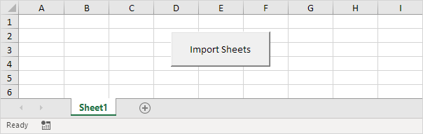
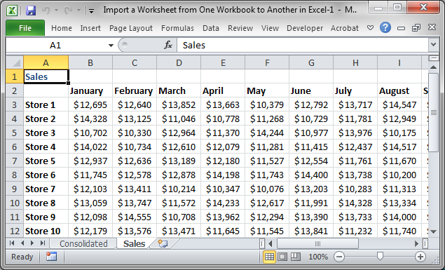
In Excel, you can quickly copy an entire worksheet from one workbook to another workbook. This allows you to import data from other workbooks with ease and without having to copy/paste everything between the worksheets.
Steps to Import a Worksheet from Another Workbook in Excel
- Make sure that you have both workbooks open, the one that has the data you want and the one to which you will import the worksheet.
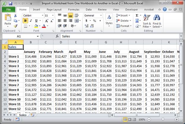
- Go to the Excel workbook that contains the worksheet that you want to export.

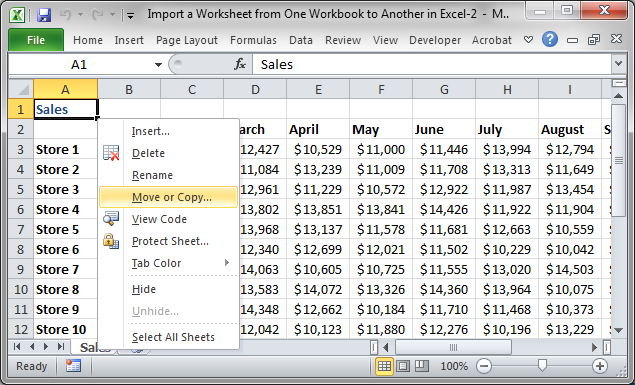
- Right-click on the tab of the worksheet that you want to export and click Move or Copy.
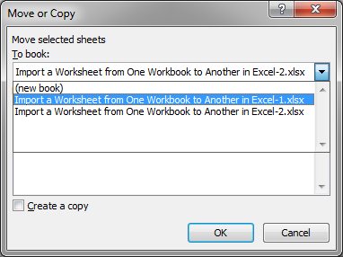
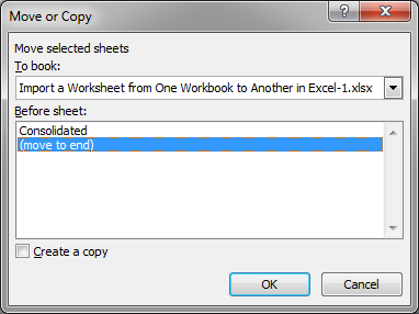
- In the window that opens up, select the workbook where you want the data to be from the To book: drop down menu:
- Choose if you want the worksheet to be placed before a specific worksheet in the new workbook or at the end of all of the worksheets:
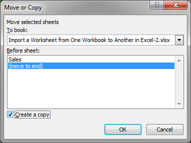
- Make sure to check the option Create a copy so that the worksheet will be copied or imported into the new workbook instead of completely moved there, which would remove the worksheet from the original workbook altogether.
- Hit OK and you will then be taken to the other workbook, the one to which the worksheet was imported.
Notes
This is a much better way of importing data between workbooks in Excel than just selecting all of the data and copy/pasting. With the method above, you are assured of importing all of the data from the worksheet and having it look exactly the same, all the while only taking a few seconds.
Make sure you check the Create a copy check box so that you will not remove the worksheet from the source workbook. This is an easy mistake to make and you might not notice it for a while.
Download the accompanying workbooks so you can test out this feature of Excel.
Question? Ask it in our Excel Forum
Excel VBA Course — From Beginner to Expert
200+ Video Lessons 50+ Hours of Instruction 200+ Excel Guides
Become a master of VBA and Macros in Excel and learn how to automate all of your tasks in Excel with this online course. (No VBA experience required.)
Источник
Import or export text (.txt or .csv) files
There are two ways to import data from a text file with Excel: you can open it in Excel, or you can import it as an external data range. To export data from Excel to a text file, use the Save As command and change the file type from the drop-down menu.
There are two commonly used text file formats:
Delimited text files (.txt), in which the TAB character (ASCII character code 009) typically separates each field of text.
Comma separated values text files (.csv), in which the comma character (,) typically separates each field of text.
You can change the separator character that is used in both delimited and .csv text files. This may be necessary to make sure that the import or export operation works the way that you want it to.
Note: You can import or export up to 1,048,576 rows and 16,384 columns.
Import a text file by opening it in Excel
You can open a text file that you created in another program as an Excel workbook by using the Open command. Opening a text file in Excel does not change the format of the file — you can see this in the Excel title bar, where the name of the file retains the text file name extension (for example, .txt or .csv).
Go to File > Open and browse to the location that contains the text file.
Select Text Files in the file type dropdown list in the Open dialog box.
Locate and double-click the text file that you want to open.
If the file is a text file (.txt), Excel starts the Import Text Wizard. When you are done with the steps, click Finish to complete the import operation. See Text Import Wizard for more information about delimiters and advanced options.
If the file is a .csv file, Excel automatically opens the text file and displays the data in a new workbook.
Note: When Excel opens a .csv file, it uses the current default data format settings to interpret how to import each column of data. If you want more flexibility in converting columns to different data formats, you can use the Import Text Wizard. For example, the format of a data column in the .csv file may be MDY, but Excel’s default data format is YMD, or you want to convert a column of numbers that contains leading zeros to text so you can preserve the leading zeros. To force Excel to run the Import Text Wizard, you can change the file name extension from .csv to .txt before you open it, or you can import a text file by connecting to it (for more information, see the following section).
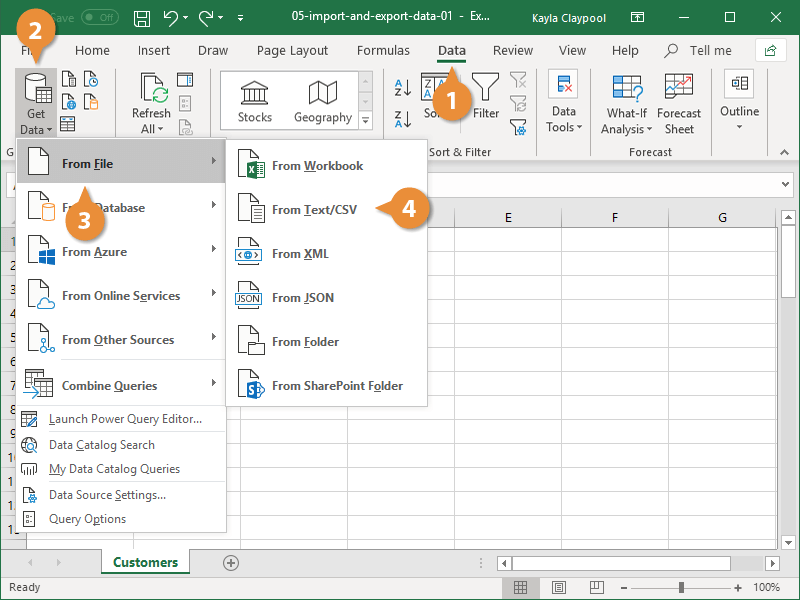
Import a text file by connecting to it (Power Query)
You can import data from a text file into an existing worksheet.
On the Data tab, in the Get & Transform Data group, click From Text/CSV.
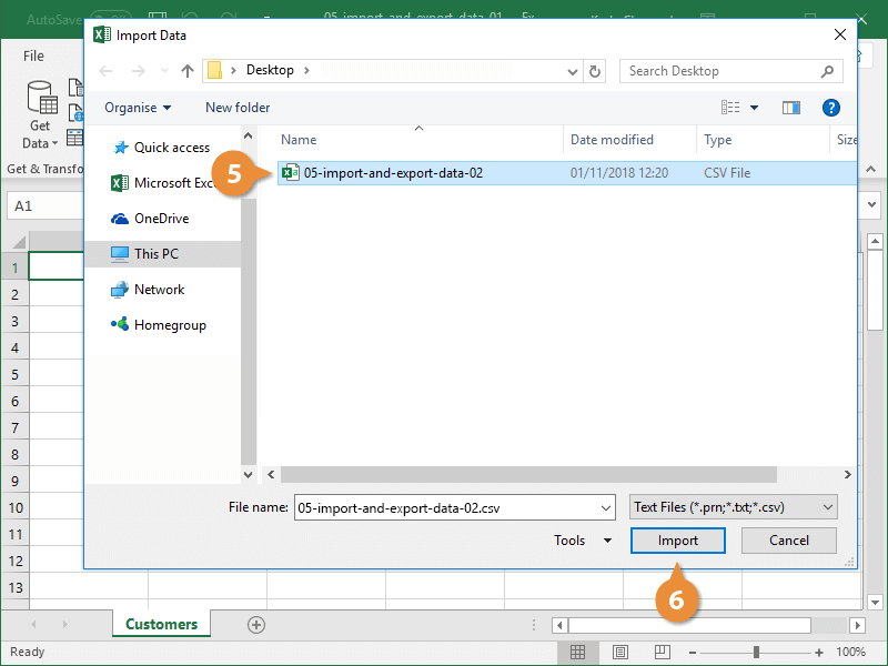
In the Import Data dialog box, locate and double-click the text file that you want to import, and click Import.
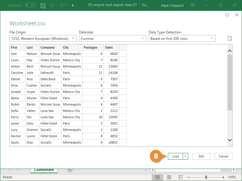
In the preview dialog box, you have several options:
Select Load if you want to load the data directly to a new worksheet.
Alternatively, select Load to if you want to load the data to a table, PivotTable/PivotChart, an existing/new Excel worksheet, or simply create a connection. You also have the choice of adding your data to the Data Model.
Select Transform Data if you want to load the data to Power Query, and edit it before bringing it to Excel.
If Excel doesn’t convert a particular column of data to the format that you want, then you can convert the data after you import it. For more information, see Convert numbers stored as text to numbers and Convert dates stored as text to dates.
Export data to a text file by saving it
You can convert an Excel worksheet to a text file by using the Save As command.
Go to File > Save As.
In the Save As dialog box, under Save as type box, choose the text file format for the worksheet; for example, click Text (Tab delimited) or CSV (Comma delimited).
Note: The different formats support different feature sets. For more information about the feature sets that are supported by the different text file formats, see File formats that are supported in Excel.
Browse to the location where you want to save the new text file, and then click Save.
A dialog box appears, reminding you that only the current worksheet will be saved to the new file. If you are certain that the current worksheet is the one that you want to save as a text file, click OK. You can save other worksheets as separate text files by repeating this procedure for each worksheet.
You may also see an alert below the ribbon that some features might be lost if you save the workbook in a CSV format.
For more information about saving files in other formats, see Save a workbook in another file format.
Import a text file by connecting to it
You can import data from a text file into an existing worksheet.
Click the cell where you want to put the data from the text file.
On the Data tab, in the Get External Data group, click From Text.
In the Import Data dialog box, locate and double-click the text file that you want to import, and click Import.
Follow the instructions in the Text Import Wizard. Click Help  on any page of the Text Import Wizard for more information about using the wizard. When you are done with the steps in the wizard, click Finish to complete the import operation.
In the Import Data dialog box, do the following:
Under Where do you want to put the data?, do one of the following:
To return the data to the location that you selected, click Existing worksheet.
To return the data to the upper-left corner of a new worksheet, click New worksheet.
Optionally, click Properties to set refresh, formatting, and layout options for the imported data.
Excel puts the external data range in the location that you specify.
If Excel does not convert a column of data to the format that you want, you can convert the data after you import it. For more information, see Convert numbers stored as text to numbers and Convert dates stored as text to dates.
Export data to a text file by saving it
You can convert an Excel worksheet to a text file by using the Save As command.
Go to File > Save As.
The Save As dialog box appears.
In the Save as type box, choose the text file format for the worksheet.
For example, click Text (Tab delimited) or CSV (Comma delimited).
Note: The different formats support different feature sets. For more information about the feature sets that are supported by the different text file formats, see File formats that are supported in Excel.
Browse to the location where you want to save the new text file, and then click Save.
A dialog box appears, reminding you that only the current worksheet will be saved to the new file. If you are certain that the current worksheet is the one that you want to save as a text file, click OK. You can save other worksheets as separate text files by repeating this procedure for each worksheet.
A second dialog box appears, reminding you that your worksheet may contain features that are not supported by text file formats. If you are interested only in saving the worksheet data into the new text file, click Yes. If you are unsure and would like to know more about which Excel features are not supported by text file formats, click Help for more information.
For more information about saving files in other formats, see Save a workbook in another file format.
The way you change the delimiter when importing is different depending on how you import the text.
If you use Get & Transform Data > From Text/CSV, after you choose the text file and click Import, choose a character to use from the list under Delimiter. You can see the effect of your new choice immediately in the data preview, so you can be sure you make the choice you want before you proceed.
If you use the Text Import Wizard to import a text file, you can change the delimiter that is used for the import operation in Step 2 of the Text Import Wizard. In this step, you can also change the way that consecutive delimiters, such as consecutive quotation marks, are handled.
See Text Import Wizard for more information about delimiters and advanced options.
If you want to use a semi-colon as the default list separator when you Save As .csv, but need to limit the change to Excel, consider changing the default decimal separator to a comma — this forces Excel to use a semi-colon for the list separator. Obviously, this will also change the way decimal numbers are displayed, so also consider changing the Thousands separator to limit any confusion.
Clear Excel Options > Advanced > Editing options > Use system separators.
Set Decimal separator to , (a comma).
Set Thousands separator to . (a period).
When you save a workbook as a .csv file, the default list separator (delimiter) is a comma. You can change this to another separator character using Windows Region settings.
Caution: Changing the Windows setting will cause a global change on your computer, affecting all applications. To only change the delimiter for Excel, see Change the default list separator for saving files as text (.csv) in Excel.
In Microsoft Windows 10, right-click the Start button, and then click Settings.
Click Time & Language, and then click Region in the left panel.
In the main panel, under Regional settings, click Additional date, time, and regional settings.
Under Region, click Change date, time, or number formats.
In the Region dialog, on the Format tab, click Additional settings.
In the Customize Format dialog, on the Numbers tab, type a character to use as the new separator in the List separator box.
In Microsoft Windows, click the Start button, and then click Control Panel.
Under Clock, Language, and Region, click Change date, time, or number formats.
In the Region dialog, on the Format tab, click Additional settings.
In the Customize Format dialog, on the Numbers tab, type a character to use as the new separator in the List separator box.
Note: After you change the list separator character for your computer, all programs use the new character as a list separator. You can change the character back to the default character by following the same procedure.
Need more help?
You can always ask an expert in the Excel Tech Community or get support in the Answers community.
Источник
Abstract: This is the first tutorial in a series designed to get you acquainted and comfortable using Excel and its built-in data mash-up and analysis features. These tutorials build and refine an Excel workbook from scratch, build a data model, then create amazing interactive reports using Power View. The tutorials are designed to demonstrate Microsoft Business Intelligence features and capabilities in Excel, PivotTables, Power Pivot, and Power View.
Note: This article describes data models in Excel 2013. However, the same data modeling and Power Pivot features introduced in Excel 2013 also apply to Excel 2016.
In these tutorials you learn how to import and explore data in Excel, build and refine a data model using Power Pivot, and create interactive reports with Power View that you can publish, protect, and share.
The tutorials in this series are the following:
-
Import Data into Excel 2013, and Create a Data Model
-
Extend Data Model relationships using Excel, Power Pivot, and DAX
-
Create Map-based Power View Reports
-
Incorporate Internet Data, and Set Power View Report Defaults
-
Power Pivot Help
-
Create Amazing Power View Reports — Part 2
In this tutorial, you start with a blank Excel workbook.
The sections in this tutorial are the following:
-
Import data from a database
-
Import data from a spreadsheet
-
Import data using copy and paste
-
Create a relationship between imported data
-
Checkpoint and Quiz
At the end of this tutorial is a quiz you can take to test your learning.
This tutorial series uses data describing Olympic Medals, hosting countries, and various Olympic sporting events. We suggest you go through each tutorial in order. Also, tutorials use Excel 2013 with Power Pivot enabled. For more information on Excel 2013, click here. For guidance on enabling Power Pivot, click here.
Import data from a database
We start this tutorial with a blank workbook. The goal in this section is to connect to an external data source, and import that data into Excel for further analysis.
Let’s start by downloading some data from the Internet. The data describes Olympic Medals, and is a Microsoft Access database.
-
Click the following links to download files we use during this tutorial series. Download each of the four files to a location that’s easily accessible, such as Downloads or My Documents, or to a new folder you create:
> OlympicMedals.accdb Access database
> OlympicSports.xlsx Excel workbook
> Population.xlsx Excel workbook
> DiscImage_table.xlsx Excel workbook -
In Excel 2013, open a blank workbook.
-
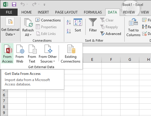
Click DATA > Get External Data > From Access. The ribbon adjusts dynamically based on the width of your workbook, so the commands on your ribbon may look slightly different from the following screens. The first screen shows the ribbon when a workbook is wide, the second image shows a workbook that has been resized to take up only a portion of the screen.
-
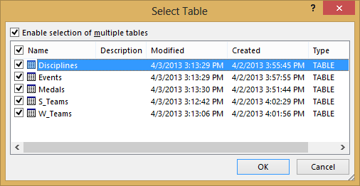
Select the OlympicMedals.accdb file you downloaded and click Open. The following Select Table window appears, displaying the tables found in the database. Tables in a database are similar to worksheets or tables in Excel. Check the Enable selection of multiple tables box, and select all the tables. Then click OK.
-
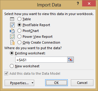
The Import Data window appears.
Note: Notice the checkbox at the bottom of the window that allows you to Add this data to the Data Model, shown in the following screen. A Data Model is created automatically when you import or work with two or more tables simultaneously. A Data Model integrates the tables, enabling extensive analysis using PivotTables, Power Pivot, and Power View. When you import tables from a database, the existing database relationships between those tables is used to create the Data Model in Excel. The Data Model is transparent in Excel, but you can view and modify it directly using the Power Pivot add-in. The Data Model is discussed in more detail later in this tutorial.
Select the PivotTable Report option, which imports the tables into Excel and prepares a PivotTable for analyzing the imported tables, and click OK.
-
Once the data is imported, a PivotTable is created using the imported tables.
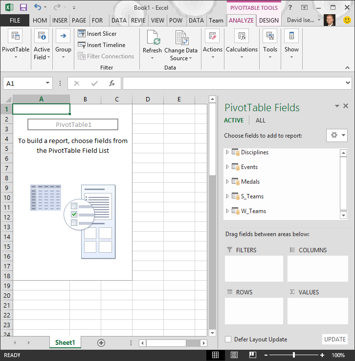
With the data imported into Excel, and the Data Model automatically created, you’re ready to explore the data.
Explore data using a PivotTable
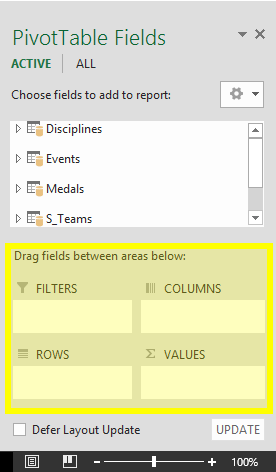
Exploring imported data is easy using a PivotTable. In a PivotTable, you drag fields (similar to columns in Excel) from tables (like the tables you just imported from the Access database) into different areas of the PivotTable to adjust how it presents your data. A PivotTable has four areas: FILTERS, COLUMNS, ROWS, and VALUES.
It might take some experimenting to determine which area a field should be dragged to. You can drag as many or few fields from your tables as you like, until the PivotTable presents your data how you want to see it. Feel free to explore by dragging fields into different areas of the PivotTable; the underlying data is not affected when you arrange fields in a PivotTable.
Let’s explore the Olympic Medals data in the PivotTable, starting with Olympic medalists organized by discipline, medal type, and the athlete’s country or region.
-
In PivotTable Fields, expand the Medals table by clicking the arrow beside it. Find the NOC_CountryRegion field in the expanded Medals table, and drag it to the COLUMNS area. NOC stands for National Olympic Committees, which is the organizational unit for a country or region.
-
Next, from the Disciplines table, drag Discipline to the ROWS area.
-
Let’s filter Disciplines to display only five sports: Archery, Diving, Fencing, Figure Skating, and Speed Skating. You can do this from within the PivotTable Fields area, or from the Row Labels filter in the PivotTable itself.
-
Click anywhere in the PivotTable to ensure the Excel PivotTable is selected. In the PivotTable Fields list, where the Disciplines table is expanded, hover over its Discipline field and a dropdown arrow appears to the right of the field. Click the dropdown, click (Select All)to remove all selections, then scroll down and select Archery, Diving, Fencing, Figure Skating, and Speed Skating. Click OK.
-
Or, in the Row Labels section of the PivotTable, click the dropdown next to Row Labels in the PivotTable, click (Select All) to remove all selections, then scroll down and select Archery, Diving, Fencing, Figure Skating, and Speed Skating. Click OK.
-
-
In PivotTable Fields, from the Medals table, drag Medal to the VALUES area. Since Values must be numeric, Excel automatically changes Medal to Count of Medal.
-
From the Medals table, select Medal again and drag it into the FILTERS area.
-
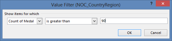
Let’s filter the PivotTable to display only those countries or regions with more than 90 total medals. Here’s how.
-
In the PivotTable, click the dropdown to the right of Column Labels.
-
Select Value Filters and select Greater Than….
-
Type 90 in the last field (on the right). Click OK.
-
Your PivotTable looks like the following screen.
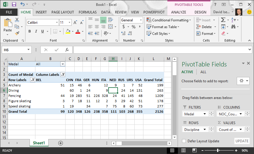
With little effort, you now have a basic PivotTable that includes fields from three different tables. What made this task so simple were the pre-existing relationships among the tables. Because table relationships existed in the source database, and because you imported all the tables in a single operation, Excel could recreate those table relationships in its Data Model.
But what if your data originates from different sources, or is imported at a later time? Typically, you can create relationships with new data based on matching columns. In the next step, you import additional tables, and learn how to create new relationships.
Import data from a spreadsheet
Now let’s import data from another source, this time from an existing workbook, then specify the relationships between our existing data and the new data. Relationships let you analyze collections of data in Excel, and create interesting and immersive visualizations from the data you import.
Let’s start by creating a blank worksheet, then import data from an Excel workbook.
-
Insert a new Excel worksheet, and name it Sports.
-
Browse to the folder that contains the downloaded sample data files, and open OlympicSports.xlsx.
-
Select and copy the data in Sheet1. If you select a cell with data, such as cell A1, you can press Ctrl + A to select all adjacent data. Close the OlympicSports.xlsx workbook.
-
On the Sports worksheet, place your cursor in cell A1 and paste the data.
-
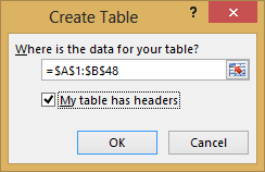
With the data still highlighted, press Ctrl + T to format the data as a table. You can also format the data as a table from the ribbon by selecting HOME > Format as Table. Since the data has headers, select My table has headers in the Create Table window that appears, as shown here.
Formatting the data as a table has many advantages. You can assign a name to a table, which makes it easy to identify. You can also establish relationships between tables, enabling exploration and analysis in PivotTables, Power Pivot, and Power View.
-
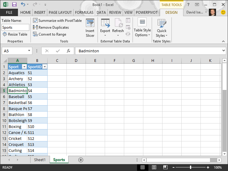
Name the table. In TABLE TOOLS > DESIGN > Properties, locate the Table Name field and type Sports. The workbook looks like the following screen.
-
Save the workbook.
Import data using copy and paste
Now that we’ve imported data from an Excel workbook, let’s import data from a table we find on a web page, or any other source from which we can copy and paste into Excel. In the following steps, you add the Olympic host cities from a table.
-
Insert a new Excel worksheet, and name it Hosts.
-
Select and copy the following table, including the table headers.
|
City |
NOC_CountryRegion |
Alpha-2 Code |
Edition |
Season |
|
Melbourne / Stockholm |
AUS |
AS |
1956 |
Summer |
|
Sydney |
AUS |
AS |
2000 |
Summer |
|
Innsbruck |
AUT |
AT |
1964 |
Winter |
|
Innsbruck |
AUT |
AT |
1976 |
Winter |
|
Antwerp |
BEL |
BE |
1920 |
Summer |
|
Antwerp |
BEL |
BE |
1920 |
Winter |
|
Montreal |
CAN |
CA |
1976 |
Summer |
|
Lake Placid |
CAN |
CA |
1980 |
Winter |
|
Calgary |
CAN |
CA |
1988 |
Winter |
|
St. Moritz |
SUI |
SZ |
1928 |
Winter |
|
St. Moritz |
SUI |
SZ |
1948 |
Winter |
|
Beijing |
CHN |
CH |
2008 |
Summer |
|
Berlin |
GER |
GM |
1936 |
Summer |
|
Garmisch-Partenkirchen |
GER |
GM |
1936 |
Winter |
|
Barcelona |
ESP |
SP |
1992 |
Summer |
|
Helsinki |
FIN |
FI |
1952 |
Summer |
|
Paris |
FRA |
FR |
1900 |
Summer |
|
Paris |
FRA |
FR |
1924 |
Summer |
|
Chamonix |
FRA |
FR |
1924 |
Winter |
|
Grenoble |
FRA |
FR |
1968 |
Winter |
|
Albertville |
FRA |
FR |
1992 |
Winter |
|
London |
GBR |
UK |
1908 |
Summer |
|
London |
GBR |
UK |
1908 |
Winter |
|
London |
GBR |
UK |
1948 |
Summer |
|
Munich |
GER |
DE |
1972 |
Summer |
|
Athens |
GRC |
GR |
2004 |
Summer |
|
Cortina d’Ampezzo |
ITA |
IT |
1956 |
Winter |
|
Rome |
ITA |
IT |
1960 |
Summer |
|
Turin |
ITA |
IT |
2006 |
Winter |
|
Tokyo |
JPN |
JA |
1964 |
Summer |
|
Sapporo |
JPN |
JA |
1972 |
Winter |
|
Nagano |
JPN |
JA |
1998 |
Winter |
|
Seoul |
KOR |
KS |
1988 |
Summer |
|
Mexico |
MEX |
MX |
1968 |
Summer |
|
Amsterdam |
NED |
NL |
1928 |
Summer |
|
Oslo |
NOR |
NO |
1952 |
Winter |
|
Lillehammer |
NOR |
NO |
1994 |
Winter |
|
Stockholm |
SWE |
SW |
1912 |
Summer |
|
St Louis |
USA |
US |
1904 |
Summer |
|
Los Angeles |
USA |
US |
1932 |
Summer |
|
Lake Placid |
USA |
US |
1932 |
Winter |
|
Squaw Valley |
USA |
US |
1960 |
Winter |
|
Moscow |
URS |
RU |
1980 |
Summer |
|
Los Angeles |
USA |
US |
1984 |
Summer |
|
Atlanta |
USA |
US |
1996 |
Summer |
|
Salt Lake City |
USA |
US |
2002 |
Winter |
|
Sarajevo |
YUG |
YU |
1984 |
Winter |
-
In Excel, place your cursor in cell A1 of the Hosts worksheet and paste the data.
-
Format the data as a table. As described earlier in this tutorial, you press Ctrl + T to format the data as a table, or from HOME > Format as Table. Since the data has headers, select My table has headers in the Create Table window that appears.
-
Name the table. In TABLE TOOLS > DESIGN > Properties locate the Table Name field, and type Hosts.
-
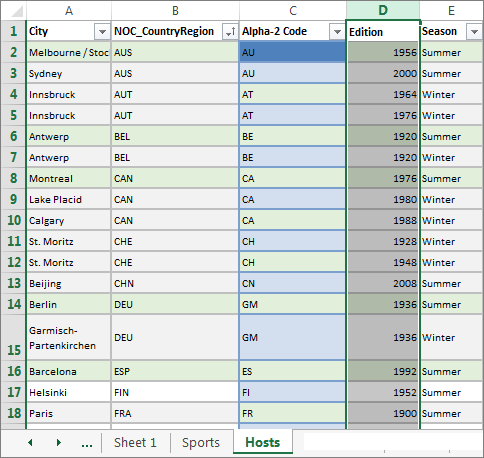
Select the Edition column, and from the HOME tab, format it as Number with 0 decimal places.
-
Save the workbook. Your workbook looks like the following screen.
Now that you have an Excel workbook with tables, you can create relationships between them. Creating relationships between tables lets you mash up the data from the two tables.
Create a relationship between imported data
You can immediately begin using fields in your PivotTable from the imported tables. If Excel can’t determine how to incorporate a field into the PivotTable, a relationship must be established with the existing Data Model. In the following steps, you learn how to create a relationship between data you imported from different sources.
-
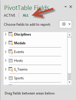
On Sheet1, at the top ofPivotTable Fields, clickAll to view the complete list of available tables, as shown in the following screen.
-
Scroll through the list to see the new tables you just added.
-
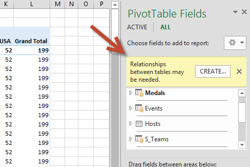
Expand Sports and select Sport to add it to the PivotTable. Notice that Excel prompts you to create a relationship, as seen in the following screen.
This notification occurs because you used fields from a table that’s not part of the underlying Data Model. One way to add a table to the Data Model is to create a relationship to a table that’s already in the Data Model. To create the relationship, one of the tables must have a column of unique, non-repeated, values. In the sample data, the Disciplines table imported from the database contains a field with sports codes, called SportID. Those same sports codes are present as a field in the Excel data we imported. Let’s create the relationship.
-
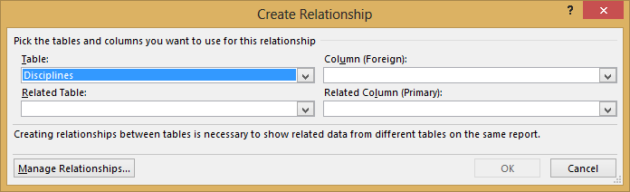
Click CREATE… in the highlighted PivotTable Fields area to open the Create Relationship dialog, as shown in the following screen.
-
In Table, choose Disciplines from the drop down list.
-
In Column (Foreign), choose SportID.
-
In Related Table, choose Sports.
-
In Related Column (Primary), choose SportID.
-
Click OK.
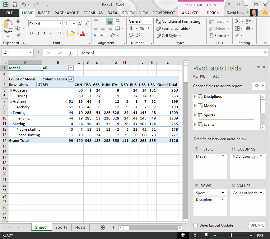
The PivotTable changes to reflect the new relationship. But the PivotTable doesn’t look right quite yet, because of the ordering of fields in the ROWS area. Discipline is a subcategory of a given sport, but since we arranged Discipline above Sport in the ROWS area, it’s not organized properly. The following screen shows this unwanted ordering.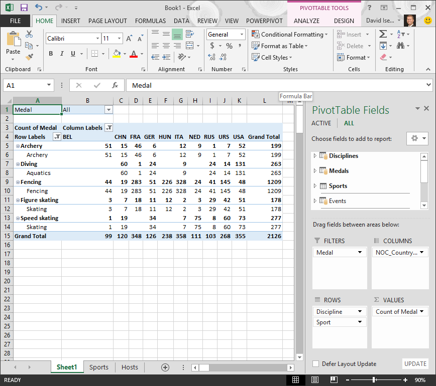
-
In the ROWS area, move Sport above Discipline. That’s much better, and the PivotTable displays the data how you want to see it, as shown in the following screen.
Behind the scenes, Excel is building a Data Model that can be used throughout the workbook, in any PivotTable, PivotChart, in Power Pivot, or any Power View report. Table relationships are the basis of a Data Model, and what determine navigation and calculation paths.
In the next tutorial, Extend Data Model relationships using Excel 2013, Power Pivot, and DAX, you build on what you learned here, and step through extending the Data Model using a powerful and visual Excel add-in called Power Pivot. You also learn how to calculate columns in a table, and use that calculated column so that an otherwise unrelated table can be added to your Data Model.
Checkpoint and Quiz
Review What You’ve Learned
You now have an Excel workbook that includes a PivotTable accessing data in multiple tables, several of which you imported separately. You learned to import from a database, from another Excel workbook, and from copying data and pasting it into Excel.
To make the data work together, you had to create a table relationship that Excel used to correlate the rows. You also learned that having columns in one table that correlate to data in another table is essential for creating relationships, and for looking up related rows.
You’re ready for the next tutorial in this series. Here’s a link:
Extend Data Model relationships using Excel 2013, Power Pivot, and DAX
QUIZ
Want to see how well you remember what you learned? Here’s your chance. The following quiz highlights features, capabilities, or requirements you learned about in this tutorial. At the bottom of the page, you’ll find the answers. Good luck!
Question 1: Why is it important to convert imported data into tables?
A: You don’t have to convert them into tables, because all imported data is automatically turned into tables.
B: If you convert imported data into tables, they will be excluded from the Data Model. Only when they’re excluded from the Data Model are they available in PivotTables, Power Pivot, and Power View.
C: If you convert imported data into tables, they can be included in the Data Model, and be made available to PivotTables, Power Pivot, and Power View.
D: You cannot convert imported data into tables.
Question 2: Which of the following data sources can you import into Excel, and include in the Data Model?
A: Access Databases, and many other databases as well.
B: Existing Excel files.
C: Anything you can copy and paste into Excel and format as a table, including data tables in websites, documents, or anything else that can be pasted into Excel.
D: All of the above
Question 3: In a PivotTable, what happens when you reorder fields in the four PivotTable Fields areas?
A: Nothing – you cannot reorder fields once you place them in the PivotTable Fields areas.
B: The PivotTable format is changed to reflect the layout, but underlying data is unaffected.
C: The PivotTable format is changed to reflect the layout, and all underlying data is permanently changed.
D: The underlying data is changed, resulting in new data sets.
Question 4: When creating a relationship between tables, what is required?
A: Neither table can have any column that contains unique, non-repeated values.
B: One table must not be part of the Excel workbook.
C: The columns must not be converted to tables.
D: None of the above is correct.
Quiz Answers
-
Correct answer: C
-
Correct answer: D
-
Correct answer: B
-
Correct answer: D
Notes: Data and images in this tutorial series are based on the following:
-
Olympics Dataset from Guardian News & Media Ltd.
-
Flag images from CIA Factbook (cia.gov)
-
Population data from The World Bank (worldbank.org)
-
Olympic Sport Pictograms by Thadius856 and Parutakupiu
Below we will look at a program in Excel VBA that imports sheets from other Excel files into one Excel file.
Download Book4.xlsx, Book5.xlsx and add them to «C:test»
Situation:
Add the following code lines to the command button:
1. First, we declare two variables of type String, a Worksheet object and one variable of type Integer.
Dim directory As String, fileName As String, sheet As Worksheet, total As Integer
2. Turn off screen updating and displaying alerts.
Application.ScreenUpdating = False
Application.DisplayAlerts = False
3. Initialize the variable directory. We use the Dir function to find the first *.xl?? file stored in this directory.
directory = «c:test»
fileName = Dir(directory & «*.xl??»)
Note: The Dir function supports the use of multiple character (*) and single character (?) wildcards to search for all different type of Excel files.
4. The variable fileName now holds the name of the first Excel file found in the directory. Add a Do While Loop.
Do While fileName <> «»
Loop
Add the following code lines (at 5, 6, 7 and to the loop.
5. There is no simple way to copy worksheets from closed Excel files. Therefore we open the Excel file.
Workbooks.Open (directory & fileName)
6. Import the sheets from the Excel file into import-sheet.xlsm.
For Each sheet In Workbooks(fileName).Worksheets
total = Workbooks(«import-sheets.xlsm»).Worksheets.count
Workbooks(fileName).Worksheets(sheet.Name).Copy _
after:=Workbooks(«import-sheets.xlsm»).Worksheets(total)
Next sheet
Explanation: the variable total holds track of the total number of worksheets of import-sheet.xlsm. We use the Copy method of the Worksheet object to copy each worksheet and paste it after the last worksheet of import-sheets.xlsm.
7. Close the Excel file.
Workbooks(fileName).Close
8. The Dir function is a special function. To get the other Excel files, you can use the Dir function again with no arguments.
fileName = Dir()
Note: When no more file names match, the Dir function returns a zero-length string («»). As a result, Excel VBA will leave the Do While loop.
9. Turn on screen updating and displaying alerts again (outside the loop).
Application.ScreenUpdating = True
Application.DisplayAlerts = True
10. Test the program.
Result:

In Excel, you can quickly copy an entire worksheet from one workbook to another workbook. This allows you to import data from other workbooks with ease and without having to copy/paste everything between the worksheets.
Steps to Import a Worksheet from Another Workbook in Excel
- Make sure that you have both workbooks open, the one that has the data you want and the one to which you will import the worksheet.
- Go to the Excel workbook that contains the worksheet that you want to export.
- Right-click on the tab of the worksheet that you want to export and click Move or Copy…
- In the window that opens up, select the workbook where you want the data to be from the To book: drop down menu:
- Choose if you want the worksheet to be placed before a specific worksheet in the new workbook or at the end of all of the worksheets:
- Make sure to check the option Create a copy so that the worksheet will be copied or imported into the new workbook instead of completely moved there, which would remove the worksheet from the original workbook altogether.
- Hit OK and you will then be taken to the other workbook, the one to which the worksheet was imported.
Notes
This is a much better way of importing data between workbooks in Excel than just selecting all of the data and copy/pasting. With the method above, you are assured of importing all of the data from the worksheet and having it look exactly the same, all the while only taking a few seconds.
Make sure you check the Create a copy check box so that you will not remove the worksheet from the source workbook. This is an easy mistake to make and you might not notice it for a while.
Download the accompanying workbooks so you can test out this feature of Excel.
![]()
Excel VBA Course — From Beginner to Expert
200+ Video Lessons
50+ Hours of Instruction
200+ Excel Guides
Become a master of VBA and Macros in Excel and learn how to automate all of your tasks in Excel with this online course. (No VBA experience required.)
View Course
Similar Content on TeachExcel
Get Data from Separate Workbooks in Excel
Tutorial: How to get data from separate workbooks in Excel. This tutorial includes an example using …
Pass Values from One Macro to Another Macro
Tutorial:
How to pass variables and values to macros. This allows you to get a result from one macr…
Pass Arguments to a Macro Called from a Button or Sheet in Excel
Tutorial: How to pass arguments and values to macros called from worksheets, buttons, and anything e…
Guide to Combine and Consolidate Data in Excel
Tutorial: Guide to combining and consolidating data in Excel. This includes consolidating data from …
Put Data into a Worksheet using a Macro in Excel
Tutorial: How to input data into cells in a worksheet from a macro.
Once you have data in your macro…
Complete Guide to Printing in Excel Macros — PrintOut Method in Excel
Macro: This free Excel macro illustrates all of the possible parameters and arguments that yo…
Subscribe for Weekly Tutorials
BONUS: subscribe now to download our Top Tutorials Ebook!
![]()
Excel VBA Course — From Beginner to Expert
200+ Video Lessons
50+ Hours of Video
200+ Excel Guides
Become a master of VBA and Macros in Excel and learn how to automate all of your tasks in Excel with this online course. (No VBA experience required.)
View Course
This is the second post of a series that covers everything about importing all files in a folder. Click here to see the series of post.
In this scenario I’ll show you to import all sheets from all excel files in a folder. If you want to follow along, download the files from this link.
Important: I’ll show how to import all sheets from all Excel files in a folder, however, it is the same process if the files contain just one sheet.
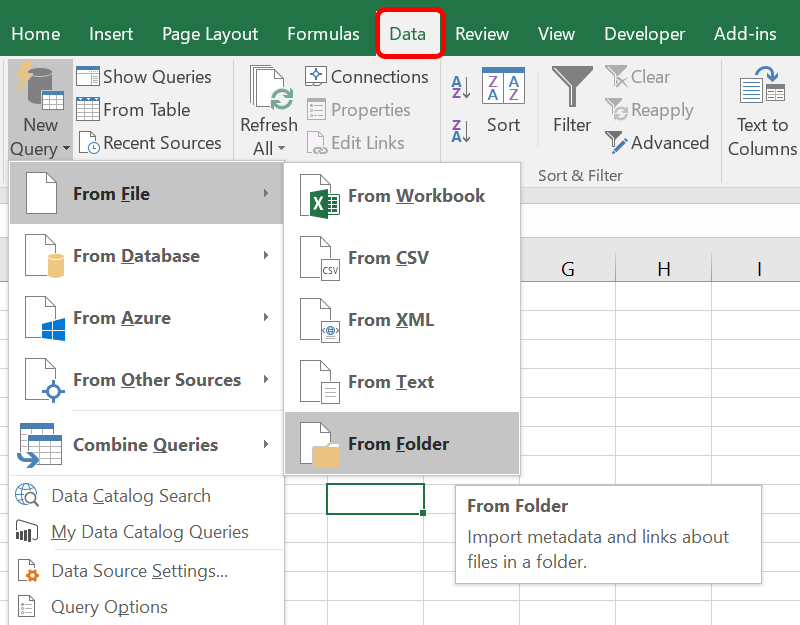
Step 1: Import the files from the desired folder
Go to Data -> New Query -> From File -> From Folder
Click on ‘Browse’ and browse for the folder that contain the files, then click OK.
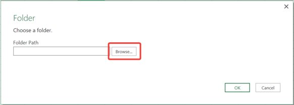
Once you click OK, press Edit on the next window.
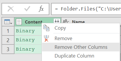
Then you’ll see a window with several details of each file in the folder such as Extension, Date accessed, Date modified, etc.
We’re only interested in the Content column, therefore, right-click on the header of the Content column and select Remove Other Columns.
The go to Add Column -> Add Custom Column

Step 2: Extract the contents from each file
In the next dialog box, type a name for the new column (e.g. FileContent) and the custom formula: =Excel.Workbook([Content], true) and click OK.
![]()
Note: The second argument of the function Excel.Workbook is to promote the headers from each sheet. If you don’t set this argument to true, you’ll have to promote the headers afterwards and then filter out the headers from the data.
Then click on the column and click OK in the Expand dialog box.

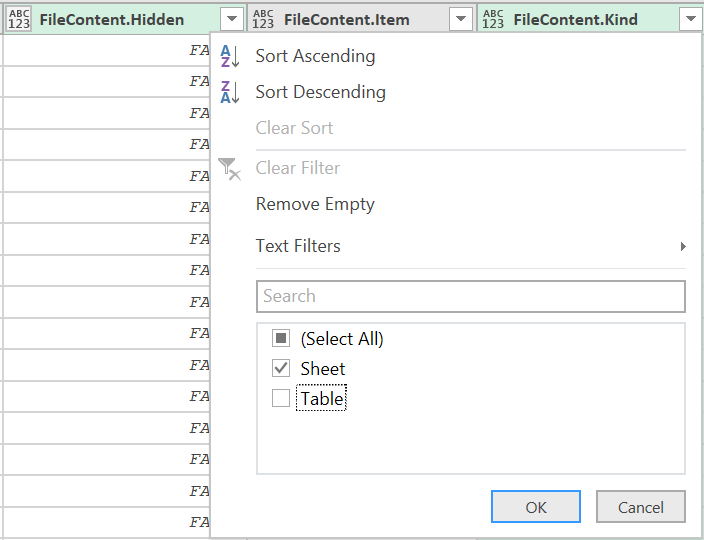
Then go to the filter button of the FileContent.Kind column, select Sheet and click OK.
Right-click the header of the FileContent.Data column and select Remove Other Columns.
Then click in the Expand button in the column FileContent.Data

In the next dialog box, make sure to uncheck the option “Use original column name as prefix” and click OK.
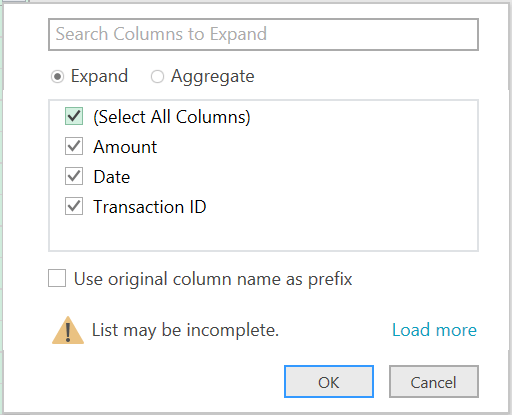
The data from ALL SHEETS from ALL FILES should be visible now. Isn’t this amazing?
Now make any further changes needed. For example, change the format of the Date column to date (Right-click the header of the Date Column, go to Change Type -> Date)
Step 3: Load the data into Excel
Go to File -> Close & Load To…

Select Table and the destination of the results (New worksheet or Existing worksheet), then click on Load.
That’s All!!!
Click here if you want to see the other posts in the series.
Want to continue learning about automating your data preparation processes?? Subscribe to the blog.
Saw this thread while looking for something else and I know it is super old, but I wanted to add my 2 cents.
NEVER USE VLOOKUP. It’s one of the worst performing formulas in excel. Use index match instead. It even works without sorting data, unless you have a -1 or 1 in the end of the match formula (explained more below)
Here is a link with the appropriate formulas.
The Sheet 2 formula would be this: =IF(A2=»»,»»,INDEX(Sheet1!B:B,MATCH($A2,Sheet1!$A:$A,0)))
- IF(A2=»»,»», means if A2 is blank, return a blank value
- INDEX(Sheet1!B:B, is saying INDEX B:B where B:B is the data you want to return. IE the name column.
- Match(A2, is saying to Match A2 which is the ID you want to return the Name for.
- Sheet1!A:A, is saying you want to match A2 to the ID column in the previous sheet
- ,0)) is specifying you want an exact value. 0 means return an exact match to A2, -1 means return smallest value greater than or equal to A2, 1 means return the largest value that is less than or equal to A2. Keep in mind -1 and 1 have to be sorted.
More information on the Index/Match formula
Other fun facts: $ means absolute in a formula. So if you specify $B$1 when filling a formula down or over keeps that same value. If you over $B1, the B remains the same across the formula, but if you fill down, the 1 increases with the row count. Likewise, if you used B$1, filling to the right will increment the B, but keep the reference of row 1.
I also included the use of indirect in the second section. What indirect does is allow you to use the text of another cell in a formula. Since I created a named range sheet1!A:A = ID, sheet1!B:B = Name, and sheet1!C:C=Price, I can use the column name to have the exact same formula, but it uses the column heading to change the search criteria.
Good luck! Hope this helps.
Excel can import and export many different file types aside from the standard .xslx format. If your data is shared between other programs, like a database, you may need to save data as a different file type or bring in files of a different file type.
Export Data
When you have data that needs to be transferred to another system, export it from Excel in a format that can be interpreted by other programs, such as a text or CSV file.
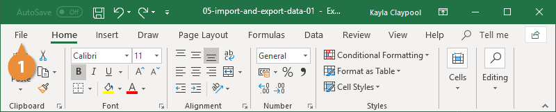
- Click the File tab.

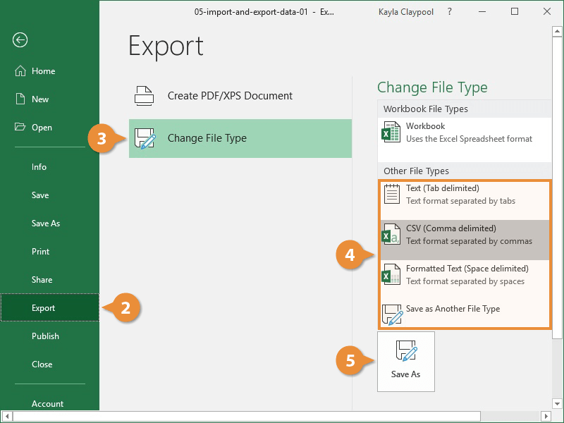
- At the left, click Export.
- Click the Change File Type.
- Under Other File Types, select a file type.
- Text (Tab delimited): The cell data will be separated by a tab.
- CSV (Comma delimited): The cell data will be separated by a comma.
- Formatted Text (space delimited): The cell data will be separated by a space.
- Save as Another File Type: Select a different file type when the Save As dialog box appears.
The file type you select will depend on what type of file is required by the program that will consume the exported data.
- Click Save As.

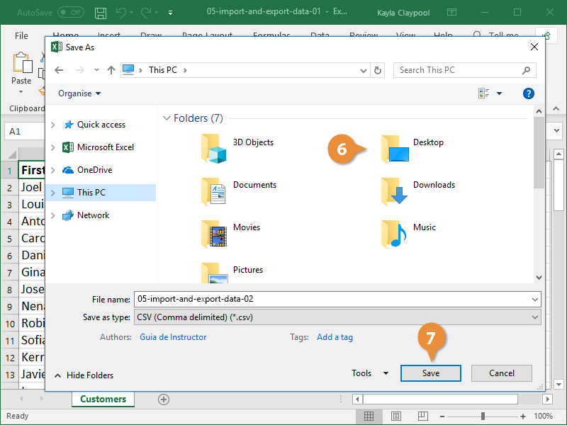
- Specify where you want to save the file.
- Click Save.
A dialog box appears stating that some of the workbook features may be lost.
- Click Yes.
Import Data
Excel can import data from external data sources including other files, databases, or web pages.
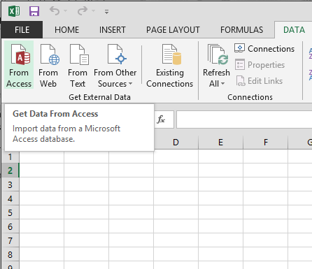
- Click the Data tab on the Ribbon..
- Click the Get Data button.
Some data sources may require special security access, and the connection process can often be very complex. Enlist the help of your organization’s technical support staff for assistance.
- Select From File.
- Select From Text/CSV.
If you have data to import from Access, the web, or another source, select one of those options in the Get External Data group instead.
- Select the file you want to import.
- Click Import.
If, while importing external data, a security notice appears saying that it is connecting to an external source that may not be safe, click OK.
- Verify the preview looks correct.
Because we’ve specified the data is separated by commas, the delimiter is already set. If you need to change it, it can be done from this menu.
- Click Load.

FREE Quick Reference
Click to Download
Free to distribute with our compliments; we hope you will consider our paid training.
In this post, we look at how to import multiple Excel files that contain multiple sheets into one Excel table.
Importing multiple files from a folder is one of the most popular functions of Power Query. A common question I get is “what about if an Excel file had multiple sheets”.
In this post, we answer that question.
You can download the files used in the tutorial to follow along.
Watch the Video
In this scenario, we have a folder that contains four Excel workbooks. Each one with training data for months of the year.
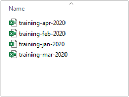
Each workbook has six sheets. Only four of those sheets (London, Birmingham, York and Reading) contain data that we want imported to the Excel table.
Import Excel Files from a Folder
Let’s start by connecting to the folder that contains the Excel files that we need.
- Click Data > Get Data > From File > From Folder.
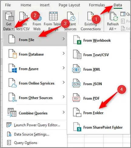
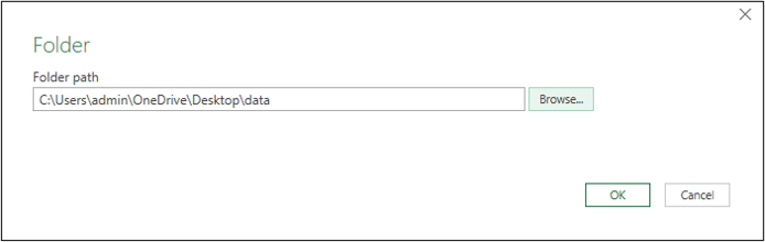
- Click the Browse button to locate the folder that contains the files. In the files provided the folder is named Data.
- Click Transform Data on the next window which lists the contents of the folder.
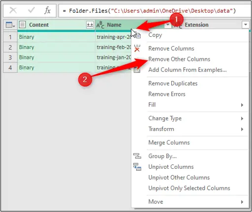
The Power Query Editor opens and shows the four Excel workbooks.
There are columns displaying the file name, extension, date created and more. We only want the Content and Name columns.
- Select the Content column, hold Ctrl and select the Name column so they are both selected. Right click and Remove Other Columns.
Create a Custom Column to Get the Sheets Data
We now need to extract the data on the sheets of each of the workbooks in that folder. For this, we will create a custom column and use a small bit of M code. Very exciting!!
- Click Add Column > Custom Column.
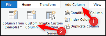
- In the Custom Column window, enter GetSheets for the column name.
- Then enter the following formula.
=Excel.Workbook([Content],true)
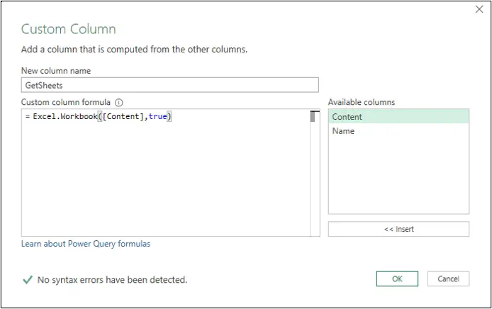
Content is the name of the header that contains the objects (sheets and tables) of the workbook. True states to use headers.
- Click Ok.
The additional column is added. This GetSheets column contains a table with information about the different objects of each workbook.
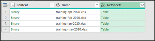
- Click the double arrow button in the GetSheets column header to extract the columns from the table. Click Ok.
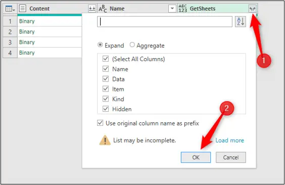
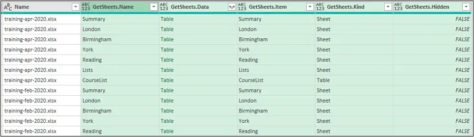
You can now see all of the sheets and tables from each workbook in the list. Information such as the object name, kind and if it is hidden or not is shown.
You can now filter out the sheets or tables that you do not want to use.
We will start by filtering out any tables, as we are only interested in the sheets, in this example.
- Click the filter arrow for the GetSheets.Kind column and uncheck the Table box. Click Ok.
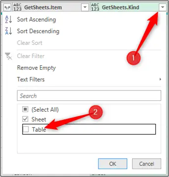
In this example, we also do not want all of the sheets. We want to exclude the Lists and Summary sheets from the data import.
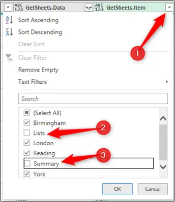
- Click the filter arrow for the GetSheets.Item column and uncheck the Lists and Summary boxes. Click Ok.
We can now remove any columns that we do not want. In this example, we will remove the Content, Name, Item, Kind and Hidden columns.
- Click on the Content column, then hold Ctrl and click the other columns. Right click and Remove Columns.
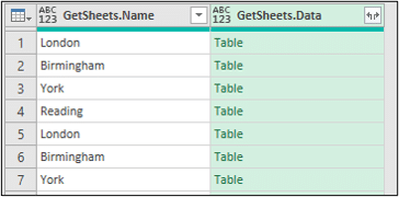
The Name column is often useful to keep, but in this example we have the date on the sheets, so the Name column offers us nothing useful.
We are left with just the sheet name and data columns.
Extract the Sheets Data
We can now extract the data for the sheets of each workbook.
- Click the double arrow button on the GetSheets.Data column.
- We will extract all of the columns but uncheck the Use original column name as prefix box.
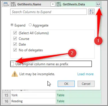
We now have all the data from those sheets and for each workbook.
To finish, we will do some final Power Query checks and changes.
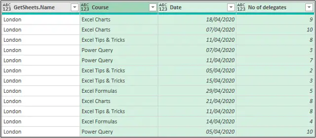
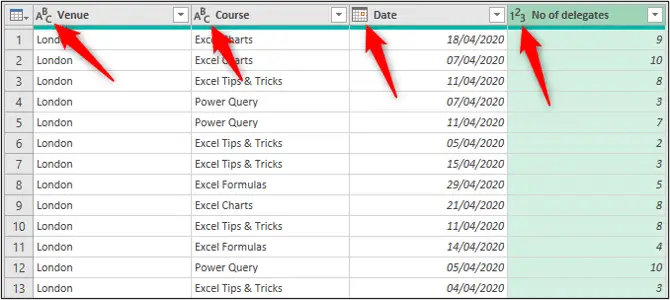
- Change the column header from GetSheets.Name to Venue.
- Change the data types, Venue to Text, Course to Text, Date to Date and No of Delegates to Whole number.
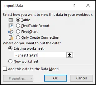
- Click Home > Close & Load list arrow > Close & Load To.
- Choose where you want to load the data. In this example, I will load it to a Table on the Existing Worksheet in range A1.
This completes the mission of importing data from multiple sheets and from multiple Excel files.
We can now continue our analysis on this data easily with formulas, PivotTables and other Excel magic.
In this article, we demonstrate how to import multiple worksheets from one Excel file, how to import multiple worksheets from multiple Excel files, and how to import a specific range of cells from an Excel sheet.
How To: Import multiple worksheets from one Excelfile
In the case where you have one Excel workbook with several sheets, you can use aDynamic Input toolto import the sheets instead of an individual Input tool for each sheet.
Note: for this method to work, the sheets of the Excel fileneed to have the same schema.

- Use anInput Tool to select Sheet Names.
- Connect a Dynamic Input tool to the Input tool.

- Configure the Dynamic Input tool to read a list of Data Sources from the Sheet Names field provided by the Input tool.
- The workflow is now configured to import the Excel sheets in a single input stream (you can see the Regions South and West from the two different Excel sheets).


How To: Import multiple worksheets from multiple Excelfiles
When you need to import multiple sheets from different excel files, you can modify the above method to work by turning it into aBatch Macro.
- Start with the same workflow from the previous example.
- Add a Control Parameter tooland a Macro Output tool to the canvas.
- Connect the Control Parameter tool to the top of the Dynamic Output and Input tools. You should see two Action tools being automatically added to the canvas between the interface tools and the standard tools.
- Connect the Macro Output tool to the output stream of the Dynamic Input tool.
Your canvas should now look like this:
- Now, we need to configure the Action Tools.
The action type should be set to «Update Value». We need only to update the file name without changing the sheet name. Therefore, for both Action Tools «Replace a specific string» should be enabled. Please note that this string should contain the path to the file to input without the extension for the sheet.
- If the Excel files have different schemas, in the interface designer we can set the macro to Auto Configure by Name or Position so that our workflow does not error out.Note: sheets within the same file will have to be the same schema.
- By default, the Interface Designer window will be displayed in the left-hand side of the Designer window.
- Click on the Cog icon in the left bar to access the Properties tab.
- Select the Output fields change based on macro’s configuration or data input option.
- By default, the Interface Designer window will be displayed in the left-hand side of the Designer window.
- You now created a Macro. In order to use it, you will need to add it to a workflow.
- Save the Macro as a Designer Macro (*.yxmc). Do not close the window with the Macro yet.
- Right-click the new workflow canvas and select Insert > Macro.
- Any Macro that is currently open in Designer can be added this way to the workflow. Note that it is also possible to create a Macro repository. This will enable to save Macros in one designated place and easily use them in workflows. See this Help Doc article.
- Finally, add a Directory tool, and connect it to the Macro’s input.
- With this configuration, you can import the Excel sheets of multiple XLSX files in the given input directory (you can see Regions North and South from the two Excel files).


Common Issues
Spoiler (Highlight to read)
The file is being used by another process
Unable to open file for read: FILEPATH. The process cannot access the file because it is being used by another process.To resolve, close any other applications (typically Microsoft Excel) that are accessing the file
Some of the columns are not imported, but in Excel the file looks fineAlteryx uses the drivers that come with Microsoft Excel to import the files. Sometimes 3rd party software does not write data in the correct Excel format.
To resolve, re-save the file in Microsoft Excel. It should now be correctly imported in Designer.
The file is being used by another processUnable to open file for read: FILEPATH. The process cannot access the file because it is being used by another process.To resolve, close any other applications (typically Microsoft Excel) that are accessing the fileSome of the columns are not imported, but in Excel the file looks fineAlteryx uses the drivers that come with Microsoft Excel to import the files. Sometimes 3rd party software does not write data in the correct Excel format.To resolve, re-save the file in Microsoft Excel. It should now be correctly imported in Designer.
How To: Input a Specific Excel Range
Another functionality of Alteryx Designer is the ability to input a data subset of an Excel file. This comes handy when working with large data.
The procedure to input an Excel range would depend on the Designer version.
Prior to 2018.1
In this example, our data starts in row 5 and column B and ends in row 7 and column D.

- Bring the Input tool into your module, then browse to the particular sheet in your Excel file that you wish to pull data from. It will look like the following image. Notice that Option #3,Table or Query, points to‘Sheet1$’, we will modify this to point to our data range.
- To edit theTable or Query, click on the button with three dots (…) on the right side of Option #3.
- Click the SQL Editor button and change the range to
SELECT * FROM 'Sheet1$B5:D7' - Click OK. Now click on theUpdate Samplelink In the Input Tool properties window to see the new range.


2018.1 and later
- In versions more recent than 2018.1, the button with three dots (…) on the right side of Option #3 cannot be used anymore.
Instead, click into the file path field, and edit it.
- Use the following syntax filepath.xlsx|||’SheetName$RangeCell1:RangeCell2′.
For example:
sample.xlsx|||'Sheet1$B5:D7'imports the Excel file sample.xlsx from Sheet1, and the range B5 : D7. Note that the value of 3. Table or Query has changed.


Additional Resources
- The Dynamic Input Tool Mastery article contains valuable insights on practical use cases of this powerful tool.
- A more general take on inputting data can be found in this insightful Knowledge Base article.
Fun Fact
Bananas grow on plants that are officially considered a herb since the stem does not contain woody tissue.