
Abstract: This is the first tutorial in a series designed to get you acquainted and comfortable using Excel and its built-in data mash-up and analysis features. These tutorials build and refine an Excel workbook from scratch, build a data model, then create amazing interactive reports using Power View. The tutorials are designed to demonstrate Microsoft Business Intelligence features and capabilities in Excel, PivotTables, Power Pivot, and Power View.
Note: This article describes data models in Excel 2013. However, the same data modeling and Power Pivot features introduced in Excel 2013 also apply to Excel 2016.
In these tutorials you learn how to import and explore data in Excel, build and refine a data model using Power Pivot, and create interactive reports with Power View that you can publish, protect, and share.
The tutorials in this series are the following:
-
Import Data into Excel 2013, and Create a Data Model
-
Extend Data Model relationships using Excel, Power Pivot, and DAX
-
Create Map-based Power View Reports
-
Incorporate Internet Data, and Set Power View Report Defaults
-
Power Pivot Help
-
Create Amazing Power View Reports — Part 2
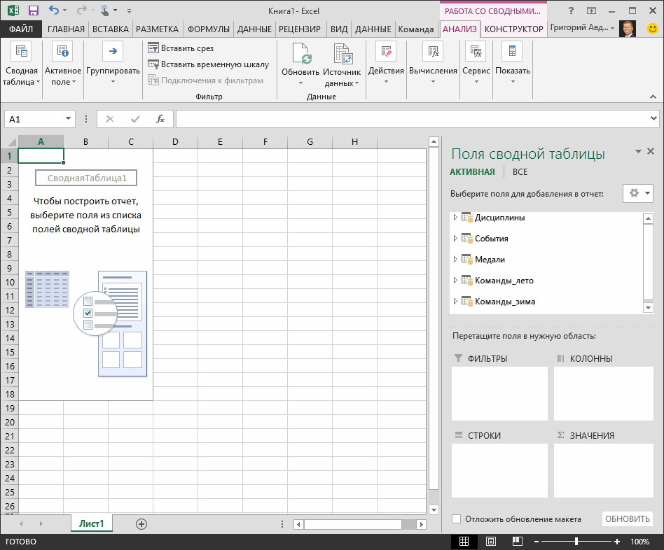
In this tutorial, you start with a blank Excel workbook.
The sections in this tutorial are the following:
-
Import data from a database
-
Import data from a spreadsheet
-
Import data using copy and paste
-
Create a relationship between imported data
-
Checkpoint and Quiz
At the end of this tutorial is a quiz you can take to test your learning.
This tutorial series uses data describing Olympic Medals, hosting countries, and various Olympic sporting events. We suggest you go through each tutorial in order. Also, tutorials use Excel 2013 with Power Pivot enabled. For more information on Excel 2013, click here. For guidance on enabling Power Pivot, click here.
Import data from a database
We start this tutorial with a blank workbook. The goal in this section is to connect to an external data source, and import that data into Excel for further analysis.
Let’s start by downloading some data from the Internet. The data describes Olympic Medals, and is a Microsoft Access database.
-
Click the following links to download files we use during this tutorial series. Download each of the four files to a location that’s easily accessible, such as Downloads or My Documents, or to a new folder you create:
> OlympicMedals.accdb Access database
> OlympicSports.xlsx Excel workbook
> Population.xlsx Excel workbook
> DiscImage_table.xlsx Excel workbook -
In Excel 2013, open a blank workbook.
-
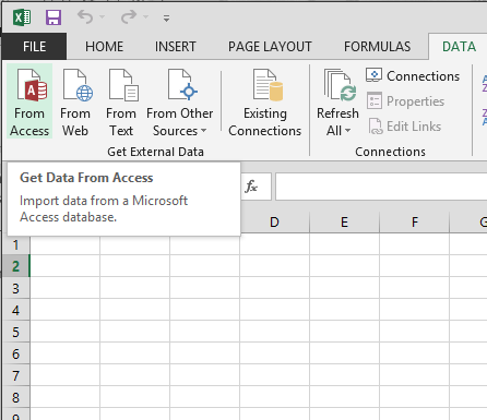
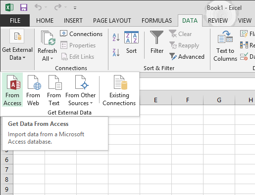
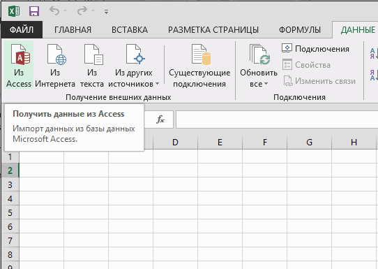
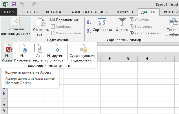
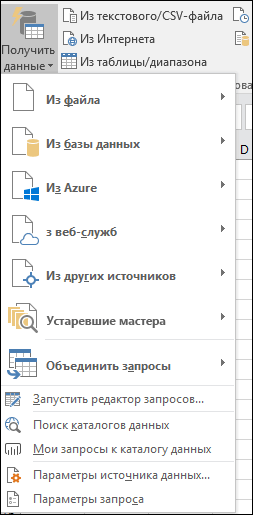
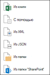
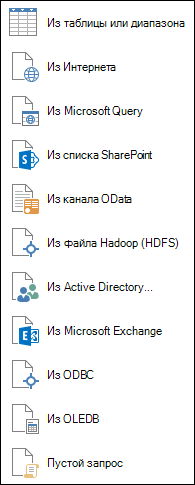
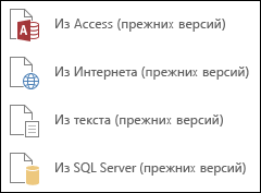
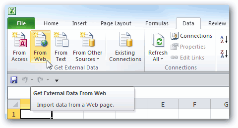
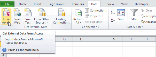
Click DATA > Get External Data > From Access. The ribbon adjusts dynamically based on the width of your workbook, so the commands on your ribbon may look slightly different from the following screens. The first screen shows the ribbon when a workbook is wide, the second image shows a workbook that has been resized to take up only a portion of the screen.

-
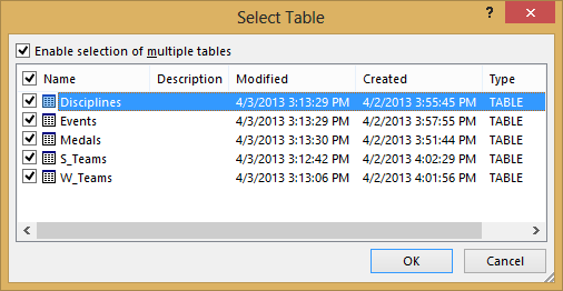
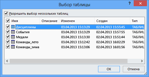
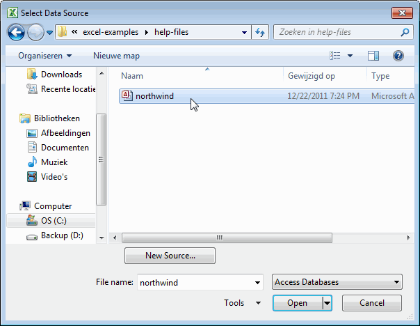
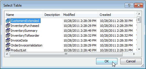
Select the OlympicMedals.accdb file you downloaded and click Open. The following Select Table window appears, displaying the tables found in the database. Tables in a database are similar to worksheets or tables in Excel. Check the Enable selection of multiple tables box, and select all the tables. Then click OK.
-
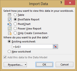
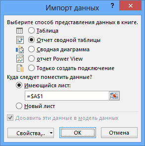
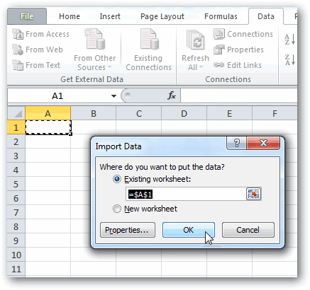
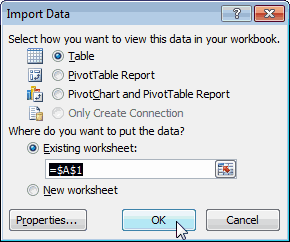
The Import Data window appears.
Note: Notice the checkbox at the bottom of the window that allows you to Add this data to the Data Model, shown in the following screen. A Data Model is created automatically when you import or work with two or more tables simultaneously. A Data Model integrates the tables, enabling extensive analysis using PivotTables, Power Pivot, and Power View. When you import tables from a database, the existing database relationships between those tables is used to create the Data Model in Excel. The Data Model is transparent in Excel, but you can view and modify it directly using the Power Pivot add-in. The Data Model is discussed in more detail later in this tutorial.
Select the PivotTable Report option, which imports the tables into Excel and prepares a PivotTable for analyzing the imported tables, and click OK.
-
Once the data is imported, a PivotTable is created using the imported tables.
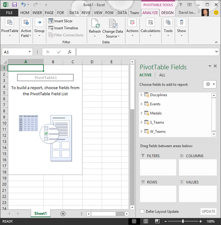
With the data imported into Excel, and the Data Model automatically created, you’re ready to explore the data.
Explore data using a PivotTable
Exploring imported data is easy using a PivotTable. In a PivotTable, you drag fields (similar to columns in Excel) from tables (like the tables you just imported from the Access database) into different areas of the PivotTable to adjust how it presents your data. A PivotTable has four areas: FILTERS, COLUMNS, ROWS, and VALUES.
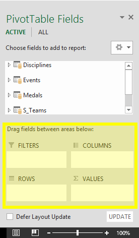
It might take some experimenting to determine which area a field should be dragged to. You can drag as many or few fields from your tables as you like, until the PivotTable presents your data how you want to see it. Feel free to explore by dragging fields into different areas of the PivotTable; the underlying data is not affected when you arrange fields in a PivotTable.
Let’s explore the Olympic Medals data in the PivotTable, starting with Olympic medalists organized by discipline, medal type, and the athlete’s country or region.
-
In PivotTable Fields, expand the Medals table by clicking the arrow beside it. Find the NOC_CountryRegion field in the expanded Medals table, and drag it to the COLUMNS area. NOC stands for National Olympic Committees, which is the organizational unit for a country or region.
-
Next, from the Disciplines table, drag Discipline to the ROWS area.
-
Let’s filter Disciplines to display only five sports: Archery, Diving, Fencing, Figure Skating, and Speed Skating. You can do this from within the PivotTable Fields area, or from the Row Labels filter in the PivotTable itself.
-
Click anywhere in the PivotTable to ensure the Excel PivotTable is selected. In the PivotTable Fields list, where the Disciplines table is expanded, hover over its Discipline field and a dropdown arrow appears to the right of the field. Click the dropdown, click (Select All)to remove all selections, then scroll down and select Archery, Diving, Fencing, Figure Skating, and Speed Skating. Click OK.
-
Or, in the Row Labels section of the PivotTable, click the dropdown next to Row Labels in the PivotTable, click (Select All) to remove all selections, then scroll down and select Archery, Diving, Fencing, Figure Skating, and Speed Skating. Click OK.
-
-
In PivotTable Fields, from the Medals table, drag Medal to the VALUES area. Since Values must be numeric, Excel automatically changes Medal to Count of Medal.
-
From the Medals table, select Medal again and drag it into the FILTERS area.
-
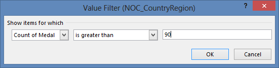
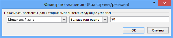
Let’s filter the PivotTable to display only those countries or regions with more than 90 total medals. Here’s how.
-
In the PivotTable, click the dropdown to the right of Column Labels.
-
Select Value Filters and select Greater Than….
-
Type 90 in the last field (on the right). Click OK.
-
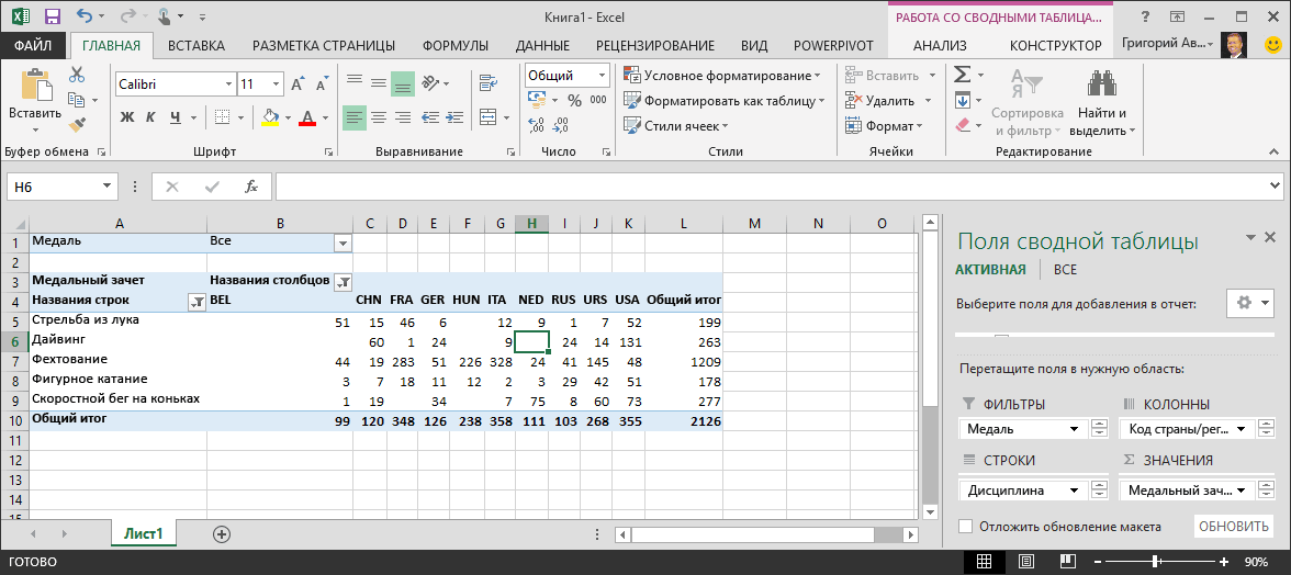
Your PivotTable looks like the following screen.
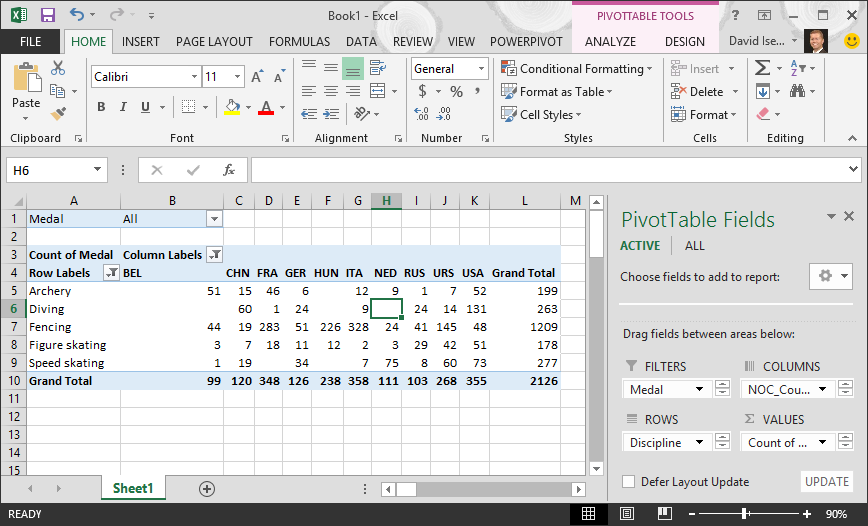
With little effort, you now have a basic PivotTable that includes fields from three different tables. What made this task so simple were the pre-existing relationships among the tables. Because table relationships existed in the source database, and because you imported all the tables in a single operation, Excel could recreate those table relationships in its Data Model.
But what if your data originates from different sources, or is imported at a later time? Typically, you can create relationships with new data based on matching columns. In the next step, you import additional tables, and learn how to create new relationships.
Import data from a spreadsheet
Now let’s import data from another source, this time from an existing workbook, then specify the relationships between our existing data and the new data. Relationships let you analyze collections of data in Excel, and create interesting and immersive visualizations from the data you import.
Let’s start by creating a blank worksheet, then import data from an Excel workbook.
-
Insert a new Excel worksheet, and name it Sports.
-
Browse to the folder that contains the downloaded sample data files, and open OlympicSports.xlsx.
-
Select and copy the data in Sheet1. If you select a cell with data, such as cell A1, you can press Ctrl + A to select all adjacent data. Close the OlympicSports.xlsx workbook.
-
On the Sports worksheet, place your cursor in cell A1 and paste the data.
-
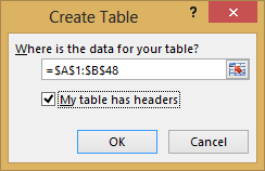
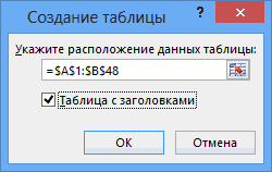
With the data still highlighted, press Ctrl + T to format the data as a table. You can also format the data as a table from the ribbon by selecting HOME > Format as Table. Since the data has headers, select My table has headers in the Create Table window that appears, as shown here.
Formatting the data as a table has many advantages. You can assign a name to a table, which makes it easy to identify. You can also establish relationships between tables, enabling exploration and analysis in PivotTables, Power Pivot, and Power View.
-
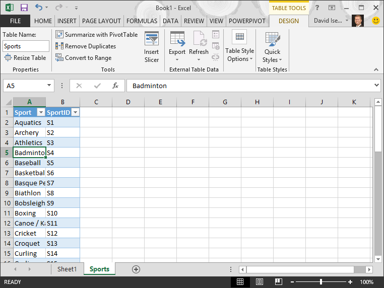
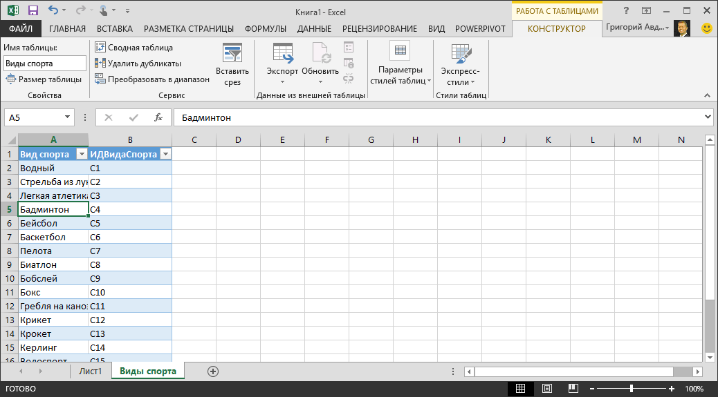
Name the table. In TABLE TOOLS > DESIGN > Properties, locate the Table Name field and type Sports. The workbook looks like the following screen.
-
Save the workbook.
Import data using copy and paste
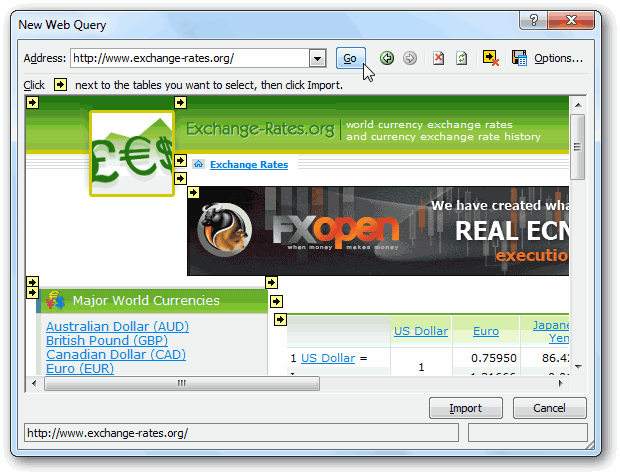
Now that we’ve imported data from an Excel workbook, let’s import data from a table we find on a web page, or any other source from which we can copy and paste into Excel. In the following steps, you add the Olympic host cities from a table.
-
Insert a new Excel worksheet, and name it Hosts.
-
Select and copy the following table, including the table headers.
|
City |
NOC_CountryRegion |
Alpha-2 Code |
Edition |
Season |
|
Melbourne / Stockholm |
AUS |
AS |
1956 |
Summer |
|
Sydney |
AUS |
AS |
2000 |
Summer |
|
Innsbruck |
AUT |
AT |
1964 |
Winter |
|
Innsbruck |
AUT |
AT |
1976 |
Winter |
|
Antwerp |
BEL |
BE |
1920 |
Summer |
|
Antwerp |
BEL |
BE |
1920 |
Winter |
|
Montreal |
CAN |
CA |
1976 |
Summer |
|
Lake Placid |
CAN |
CA |
1980 |
Winter |
|
Calgary |
CAN |
CA |
1988 |
Winter |
|
St. Moritz |
SUI |
SZ |
1928 |
Winter |
|
St. Moritz |
SUI |
SZ |
1948 |
Winter |
|
Beijing |
CHN |
CH |
2008 |
Summer |
|
Berlin |
GER |
GM |
1936 |
Summer |
|
Garmisch-Partenkirchen |
GER |
GM |
1936 |
Winter |
|
Barcelona |
ESP |
SP |
1992 |
Summer |
|
Helsinki |
FIN |
FI |
1952 |
Summer |
|
Paris |
FRA |
FR |
1900 |
Summer |
|
Paris |
FRA |
FR |
1924 |
Summer |
|
Chamonix |
FRA |
FR |
1924 |
Winter |
|
Grenoble |
FRA |
FR |
1968 |
Winter |
|
Albertville |
FRA |
FR |
1992 |
Winter |
|
London |
GBR |
UK |
1908 |
Summer |
|
London |
GBR |
UK |
1908 |
Winter |
|
London |
GBR |
UK |
1948 |
Summer |
|
Munich |
GER |
DE |
1972 |
Summer |
|
Athens |
GRC |
GR |
2004 |
Summer |
|
Cortina d’Ampezzo |
ITA |
IT |
1956 |
Winter |
|
Rome |
ITA |
IT |
1960 |
Summer |
|
Turin |
ITA |
IT |
2006 |
Winter |
|
Tokyo |
JPN |
JA |
1964 |
Summer |
|
Sapporo |
JPN |
JA |
1972 |
Winter |
|
Nagano |
JPN |
JA |
1998 |
Winter |
|
Seoul |
KOR |
KS |
1988 |
Summer |
|
Mexico |
MEX |
MX |
1968 |
Summer |
|
Amsterdam |
NED |
NL |
1928 |
Summer |
|
Oslo |
NOR |
NO |
1952 |
Winter |
|
Lillehammer |
NOR |
NO |
1994 |
Winter |
|
Stockholm |
SWE |
SW |
1912 |
Summer |
|
St Louis |
USA |
US |
1904 |
Summer |
|
Los Angeles |
USA |
US |
1932 |
Summer |
|
Lake Placid |
USA |
US |
1932 |
Winter |
|
Squaw Valley |
USA |
US |
1960 |
Winter |
|
Moscow |
URS |
RU |
1980 |
Summer |
|
Los Angeles |
USA |
US |
1984 |
Summer |
|
Atlanta |
USA |
US |
1996 |
Summer |
|
Salt Lake City |
USA |
US |
2002 |
Winter |
|
Sarajevo |
YUG |
YU |
1984 |
Winter |
-
In Excel, place your cursor in cell A1 of the Hosts worksheet and paste the data.
-
Format the data as a table. As described earlier in this tutorial, you press Ctrl + T to format the data as a table, or from HOME > Format as Table. Since the data has headers, select My table has headers in the Create Table window that appears.
-
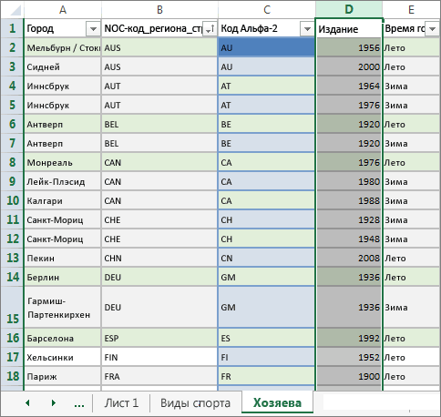
Name the table. In TABLE TOOLS > DESIGN > Properties locate the Table Name field, and type Hosts.
-
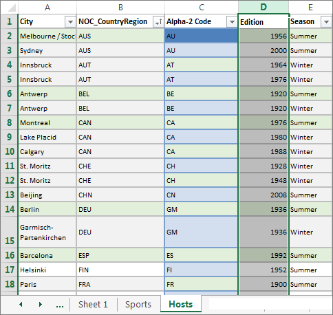
Select the Edition column, and from the HOME tab, format it as Number with 0 decimal places.
-
Save the workbook. Your workbook looks like the following screen.
Now that you have an Excel workbook with tables, you can create relationships between them. Creating relationships between tables lets you mash up the data from the two tables.
Create a relationship between imported data
You can immediately begin using fields in your PivotTable from the imported tables. If Excel can’t determine how to incorporate a field into the PivotTable, a relationship must be established with the existing Data Model. In the following steps, you learn how to create a relationship between data you imported from different sources.
-
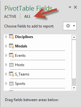
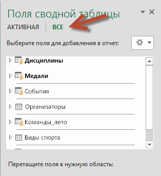
On Sheet1, at the top ofPivotTable Fields, clickAll to view the complete list of available tables, as shown in the following screen.
-
Scroll through the list to see the new tables you just added.
-
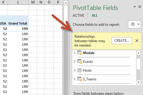
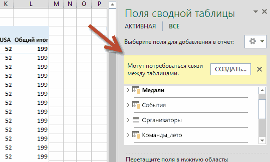
Expand Sports and select Sport to add it to the PivotTable. Notice that Excel prompts you to create a relationship, as seen in the following screen.
This notification occurs because you used fields from a table that’s not part of the underlying Data Model. One way to add a table to the Data Model is to create a relationship to a table that’s already in the Data Model. To create the relationship, one of the tables must have a column of unique, non-repeated, values. In the sample data, the Disciplines table imported from the database contains a field with sports codes, called SportID. Those same sports codes are present as a field in the Excel data we imported. Let’s create the relationship.
-
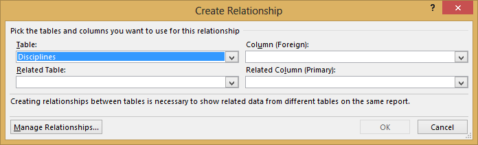
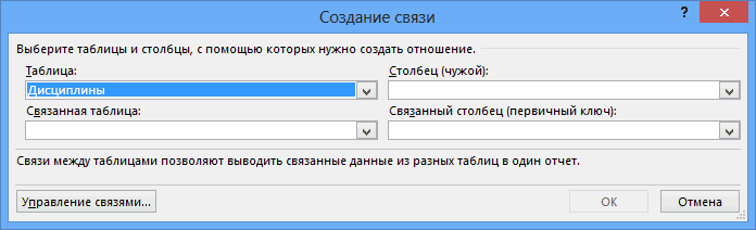
Click CREATE… in the highlighted PivotTable Fields area to open the Create Relationship dialog, as shown in the following screen.
-
In Table, choose Disciplines from the drop down list.
-
In Column (Foreign), choose SportID.
-
In Related Table, choose Sports.
-
In Related Column (Primary), choose SportID.
-
Click OK.
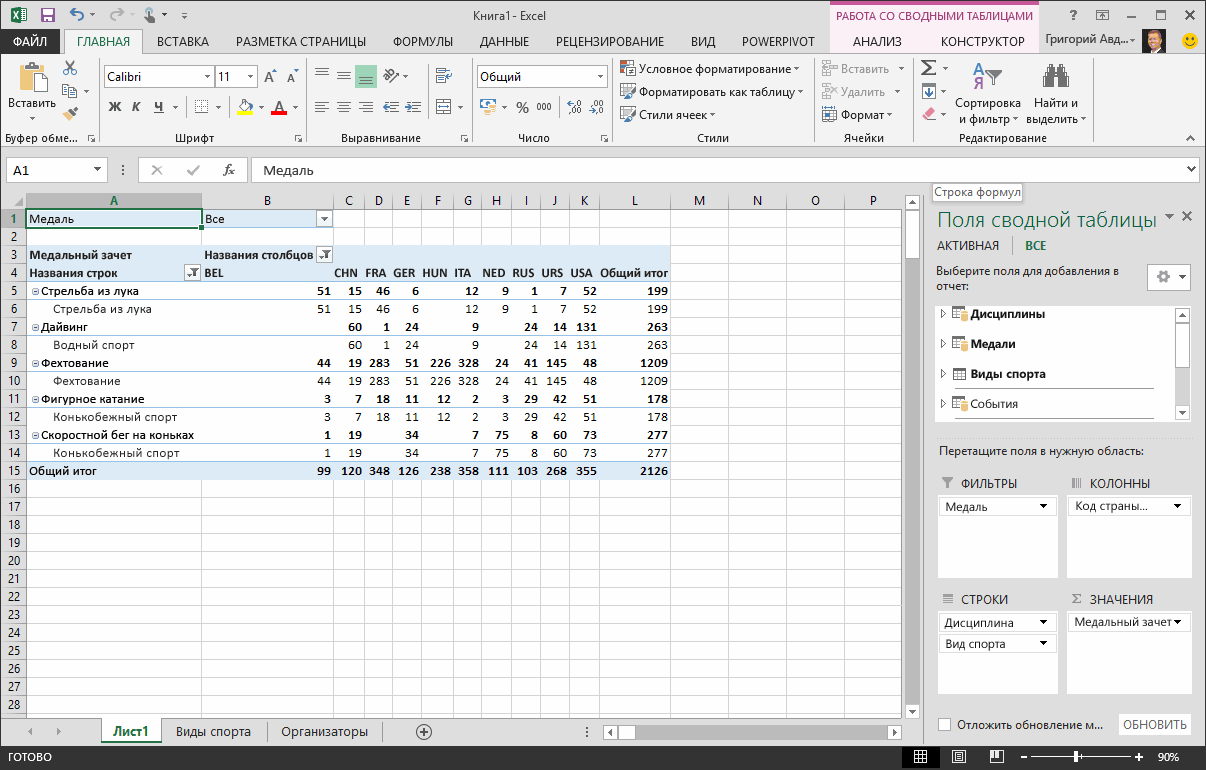
The PivotTable changes to reflect the new relationship. But the PivotTable doesn’t look right quite yet, because of the ordering of fields in the ROWS area. Discipline is a subcategory of a given sport, but since we arranged Discipline above Sport in the ROWS area, it’s not organized properly. The following screen shows this unwanted ordering.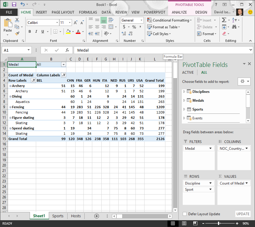
-
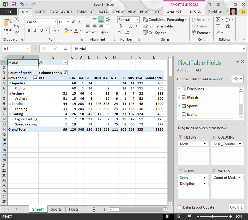
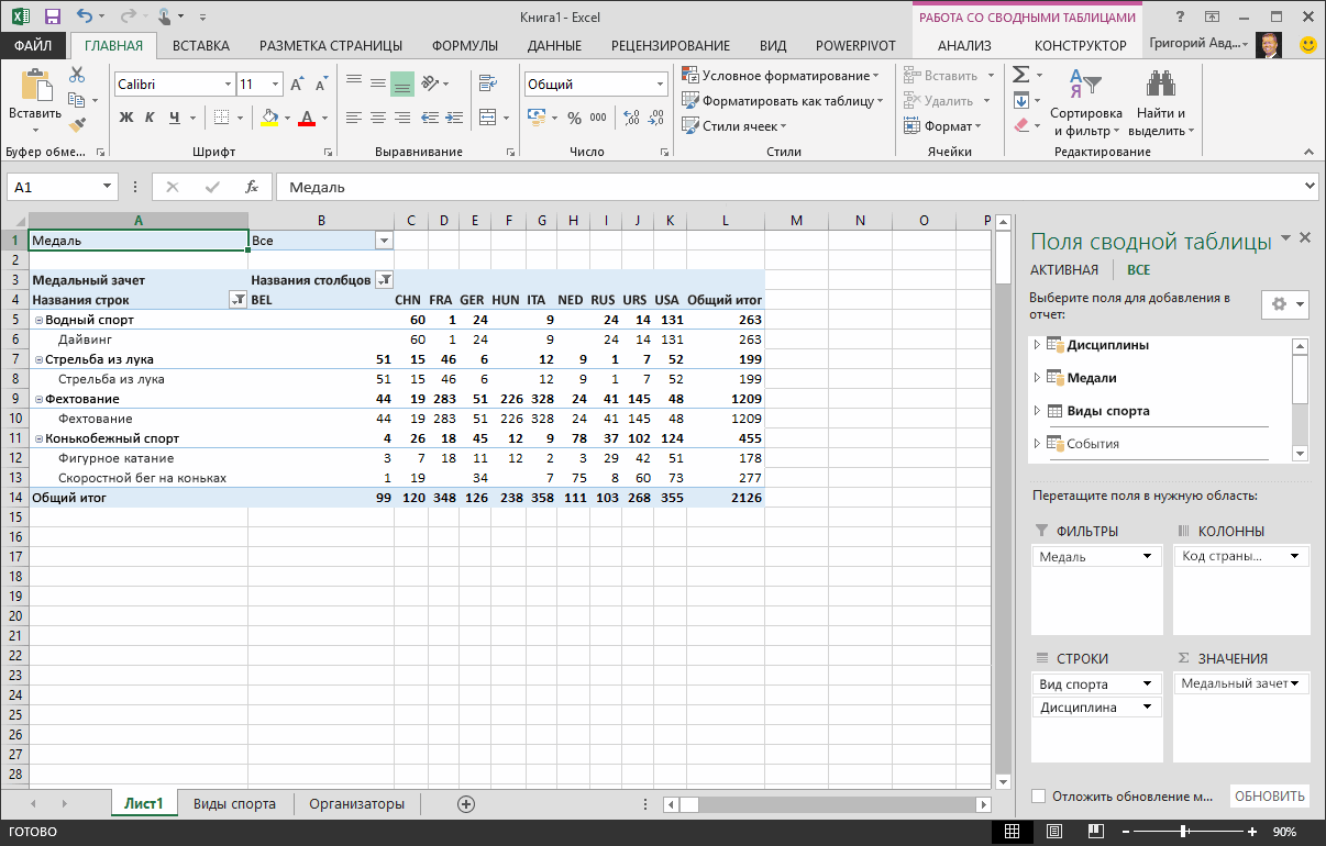
In the ROWS area, move Sport above Discipline. That’s much better, and the PivotTable displays the data how you want to see it, as shown in the following screen.
Behind the scenes, Excel is building a Data Model that can be used throughout the workbook, in any PivotTable, PivotChart, in Power Pivot, or any Power View report. Table relationships are the basis of a Data Model, and what determine navigation and calculation paths.
In the next tutorial, Extend Data Model relationships using Excel 2013, Power Pivot, and DAX, you build on what you learned here, and step through extending the Data Model using a powerful and visual Excel add-in called Power Pivot. You also learn how to calculate columns in a table, and use that calculated column so that an otherwise unrelated table can be added to your Data Model.
Checkpoint and Quiz
Review What You’ve Learned
You now have an Excel workbook that includes a PivotTable accessing data in multiple tables, several of which you imported separately. You learned to import from a database, from another Excel workbook, and from copying data and pasting it into Excel.
To make the data work together, you had to create a table relationship that Excel used to correlate the rows. You also learned that having columns in one table that correlate to data in another table is essential for creating relationships, and for looking up related rows.
You’re ready for the next tutorial in this series. Here’s a link:
Extend Data Model relationships using Excel 2013, Power Pivot, and DAX
QUIZ
Want to see how well you remember what you learned? Here’s your chance. The following quiz highlights features, capabilities, or requirements you learned about in this tutorial. At the bottom of the page, you’ll find the answers. Good luck!
Question 1: Why is it important to convert imported data into tables?
A: You don’t have to convert them into tables, because all imported data is automatically turned into tables.
B: If you convert imported data into tables, they will be excluded from the Data Model. Only when they’re excluded from the Data Model are they available in PivotTables, Power Pivot, and Power View.
C: If you convert imported data into tables, they can be included in the Data Model, and be made available to PivotTables, Power Pivot, and Power View.
D: You cannot convert imported data into tables.
Question 2: Which of the following data sources can you import into Excel, and include in the Data Model?
A: Access Databases, and many other databases as well.
B: Existing Excel files.
C: Anything you can copy and paste into Excel and format as a table, including data tables in websites, documents, or anything else that can be pasted into Excel.
D: All of the above
Question 3: In a PivotTable, what happens when you reorder fields in the four PivotTable Fields areas?
A: Nothing – you cannot reorder fields once you place them in the PivotTable Fields areas.
B: The PivotTable format is changed to reflect the layout, but underlying data is unaffected.
C: The PivotTable format is changed to reflect the layout, and all underlying data is permanently changed.
D: The underlying data is changed, resulting in new data sets.
Question 4: When creating a relationship between tables, what is required?
A: Neither table can have any column that contains unique, non-repeated values.
B: One table must not be part of the Excel workbook.
C: The columns must not be converted to tables.
D: None of the above is correct.
Quiz Answers
-
Correct answer: C
-
Correct answer: D
-
Correct answer: B
-
Correct answer: D
Notes: Data and images in this tutorial series are based on the following:
-
Olympics Dataset from Guardian News & Media Ltd.
-
Flag images from CIA Factbook (cia.gov)
-
Population data from The World Bank (worldbank.org)
-
Olympic Sport Pictograms by Thadius856 and Parutakupiu
Abstract: This is the first tutorial in a series designed to get you acquainted and comfortable using Excel and its built-in data mash-up and analysis features. These tutorials build and refine an Excel workbook from scratch, build a data model, then create amazing interactive reports using Power View. The tutorials are designed to demonstrate Microsoft Business Intelligence features and capabilities in Excel, PivotTables, Power Pivot, and Power View.
Note: This article describes data models in Excel 2013. However, the same data modeling and Power Pivot features introduced in Excel 2013 also apply to Excel 2016.
In these tutorials you learn how to import and explore data in Excel, build and refine a data model using Power Pivot, and create interactive reports with Power View that you can publish, protect, and share.
The tutorials in this series are the following:
-
Import Data into Excel 2013, and Create a Data Model
-
Extend Data Model relationships using Excel, Power Pivot, and DAX
-
Create Map-based Power View Reports
-
Incorporate Internet Data, and Set Power View Report Defaults
-
Power Pivot Help
-
Create Amazing Power View Reports — Part 2
In this tutorial, you start with a blank Excel workbook.
The sections in this tutorial are the following:
-
Import data from a database
-
Import data from a spreadsheet
-
Import data using copy and paste
-
Create a relationship between imported data
-
Checkpoint and Quiz
At the end of this tutorial is a quiz you can take to test your learning.
This tutorial series uses data describing Olympic Medals, hosting countries, and various Olympic sporting events. We suggest you go through each tutorial in order. Also, tutorials use Excel 2013 with Power Pivot enabled. For more information on Excel 2013, click here. For guidance on enabling Power Pivot, click here.
Import data from a database
We start this tutorial with a blank workbook. The goal in this section is to connect to an external data source, and import that data into Excel for further analysis.
Let’s start by downloading some data from the Internet. The data describes Olympic Medals, and is a Microsoft Access database.
-
Click the following links to download files we use during this tutorial series. Download each of the four files to a location that’s easily accessible, such as Downloads or My Documents, or to a new folder you create:
> OlympicMedals.accdb Access database
> OlympicSports.xlsx Excel workbook
> Population.xlsx Excel workbook
> DiscImage_table.xlsx Excel workbook -
In Excel 2013, open a blank workbook.
-
Click DATA > Get External Data > From Access. The ribbon adjusts dynamically based on the width of your workbook, so the commands on your ribbon may look slightly different from the following screens. The first screen shows the ribbon when a workbook is wide, the second image shows a workbook that has been resized to take up only a portion of the screen.
-
Select the OlympicMedals.accdb file you downloaded and click Open. The following Select Table window appears, displaying the tables found in the database. Tables in a database are similar to worksheets or tables in Excel. Check the Enable selection of multiple tables box, and select all the tables. Then click OK.
-
The Import Data window appears.
Note: Notice the checkbox at the bottom of the window that allows you to Add this data to the Data Model, shown in the following screen. A Data Model is created automatically when you import or work with two or more tables simultaneously. A Data Model integrates the tables, enabling extensive analysis using PivotTables, Power Pivot, and Power View. When you import tables from a database, the existing database relationships between those tables is used to create the Data Model in Excel. The Data Model is transparent in Excel, but you can view and modify it directly using the Power Pivot add-in. The Data Model is discussed in more detail later in this tutorial.
Select the PivotTable Report option, which imports the tables into Excel and prepares a PivotTable for analyzing the imported tables, and click OK.
-
Once the data is imported, a PivotTable is created using the imported tables.
With the data imported into Excel, and the Data Model automatically created, you’re ready to explore the data.
Explore data using a PivotTable
Exploring imported data is easy using a PivotTable. In a PivotTable, you drag fields (similar to columns in Excel) from tables (like the tables you just imported from the Access database) into different areas of the PivotTable to adjust how it presents your data. A PivotTable has four areas: FILTERS, COLUMNS, ROWS, and VALUES.
It might take some experimenting to determine which area a field should be dragged to. You can drag as many or few fields from your tables as you like, until the PivotTable presents your data how you want to see it. Feel free to explore by dragging fields into different areas of the PivotTable; the underlying data is not affected when you arrange fields in a PivotTable.
Let’s explore the Olympic Medals data in the PivotTable, starting with Olympic medalists organized by discipline, medal type, and the athlete’s country or region.
-
In PivotTable Fields, expand the Medals table by clicking the arrow beside it. Find the NOC_CountryRegion field in the expanded Medals table, and drag it to the COLUMNS area. NOC stands for National Olympic Committees, which is the organizational unit for a country or region.
-
Next, from the Disciplines table, drag Discipline to the ROWS area.
-
Let’s filter Disciplines to display only five sports: Archery, Diving, Fencing, Figure Skating, and Speed Skating. You can do this from within the PivotTable Fields area, or from the Row Labels filter in the PivotTable itself.
-
Click anywhere in the PivotTable to ensure the Excel PivotTable is selected. In the PivotTable Fields list, where the Disciplines table is expanded, hover over its Discipline field and a dropdown arrow appears to the right of the field. Click the dropdown, click (Select All)to remove all selections, then scroll down and select Archery, Diving, Fencing, Figure Skating, and Speed Skating. Click OK.
-
Or, in the Row Labels section of the PivotTable, click the dropdown next to Row Labels in the PivotTable, click (Select All) to remove all selections, then scroll down and select Archery, Diving, Fencing, Figure Skating, and Speed Skating. Click OK.
-
-
In PivotTable Fields, from the Medals table, drag Medal to the VALUES area. Since Values must be numeric, Excel automatically changes Medal to Count of Medal.
-
From the Medals table, select Medal again and drag it into the FILTERS area.
-
Let’s filter the PivotTable to display only those countries or regions with more than 90 total medals. Here’s how.
-
In the PivotTable, click the dropdown to the right of Column Labels.
-
Select Value Filters and select Greater Than….
-
Type 90 in the last field (on the right). Click OK.
-
Your PivotTable looks like the following screen.
With little effort, you now have a basic PivotTable that includes fields from three different tables. What made this task so simple were the pre-existing relationships among the tables. Because table relationships existed in the source database, and because you imported all the tables in a single operation, Excel could recreate those table relationships in its Data Model.
But what if your data originates from different sources, or is imported at a later time? Typically, you can create relationships with new data based on matching columns. In the next step, you import additional tables, and learn how to create new relationships.
Import data from a spreadsheet
Now let’s import data from another source, this time from an existing workbook, then specify the relationships between our existing data and the new data. Relationships let you analyze collections of data in Excel, and create interesting and immersive visualizations from the data you import.
Let’s start by creating a blank worksheet, then import data from an Excel workbook.
-
Insert a new Excel worksheet, and name it Sports.
-
Browse to the folder that contains the downloaded sample data files, and open OlympicSports.xlsx.
-
Select and copy the data in Sheet1. If you select a cell with data, such as cell A1, you can press Ctrl + A to select all adjacent data. Close the OlympicSports.xlsx workbook.
-
On the Sports worksheet, place your cursor in cell A1 and paste the data.
-
With the data still highlighted, press Ctrl + T to format the data as a table. You can also format the data as a table from the ribbon by selecting HOME > Format as Table. Since the data has headers, select My table has headers in the Create Table window that appears, as shown here.
Formatting the data as a table has many advantages. You can assign a name to a table, which makes it easy to identify. You can also establish relationships between tables, enabling exploration and analysis in PivotTables, Power Pivot, and Power View.
-
Name the table. In TABLE TOOLS > DESIGN > Properties, locate the Table Name field and type Sports. The workbook looks like the following screen.
-
Save the workbook.
Import data using copy and paste
Now that we’ve imported data from an Excel workbook, let’s import data from a table we find on a web page, or any other source from which we can copy and paste into Excel. In the following steps, you add the Olympic host cities from a table.
-
Insert a new Excel worksheet, and name it Hosts.
-
Select and copy the following table, including the table headers.
|
City |
NOC_CountryRegion |
Alpha-2 Code |
Edition |
Season |
|
Melbourne / Stockholm |
AUS |
AS |
1956 |
Summer |
|
Sydney |
AUS |
AS |
2000 |
Summer |
|
Innsbruck |
AUT |
AT |
1964 |
Winter |
|
Innsbruck |
AUT |
AT |
1976 |
Winter |
|
Antwerp |
BEL |
BE |
1920 |
Summer |
|
Antwerp |
BEL |
BE |
1920 |
Winter |
|
Montreal |
CAN |
CA |
1976 |
Summer |
|
Lake Placid |
CAN |
CA |
1980 |
Winter |
|
Calgary |
CAN |
CA |
1988 |
Winter |
|
St. Moritz |
SUI |
SZ |
1928 |
Winter |
|
St. Moritz |
SUI |
SZ |
1948 |
Winter |
|
Beijing |
CHN |
CH |
2008 |
Summer |
|
Berlin |
GER |
GM |
1936 |
Summer |
|
Garmisch-Partenkirchen |
GER |
GM |
1936 |
Winter |
|
Barcelona |
ESP |
SP |
1992 |
Summer |
|
Helsinki |
FIN |
FI |
1952 |
Summer |
|
Paris |
FRA |
FR |
1900 |
Summer |
|
Paris |
FRA |
FR |
1924 |
Summer |
|
Chamonix |
FRA |
FR |
1924 |
Winter |
|
Grenoble |
FRA |
FR |
1968 |
Winter |
|
Albertville |
FRA |
FR |
1992 |
Winter |
|
London |
GBR |
UK |
1908 |
Summer |
|
London |
GBR |
UK |
1908 |
Winter |
|
London |
GBR |
UK |
1948 |
Summer |
|
Munich |
GER |
DE |
1972 |
Summer |
|
Athens |
GRC |
GR |
2004 |
Summer |
|
Cortina d’Ampezzo |
ITA |
IT |
1956 |
Winter |
|
Rome |
ITA |
IT |
1960 |
Summer |
|
Turin |
ITA |
IT |
2006 |
Winter |
|
Tokyo |
JPN |
JA |
1964 |
Summer |
|
Sapporo |
JPN |
JA |
1972 |
Winter |
|
Nagano |
JPN |
JA |
1998 |
Winter |
|
Seoul |
KOR |
KS |
1988 |
Summer |
|
Mexico |
MEX |
MX |
1968 |
Summer |
|
Amsterdam |
NED |
NL |
1928 |
Summer |
|
Oslo |
NOR |
NO |
1952 |
Winter |
|
Lillehammer |
NOR |
NO |
1994 |
Winter |
|
Stockholm |
SWE |
SW |
1912 |
Summer |
|
St Louis |
USA |
US |
1904 |
Summer |
|
Los Angeles |
USA |
US |
1932 |
Summer |
|
Lake Placid |
USA |
US |
1932 |
Winter |
|
Squaw Valley |
USA |
US |
1960 |
Winter |
|
Moscow |
URS |
RU |
1980 |
Summer |
|
Los Angeles |
USA |
US |
1984 |
Summer |
|
Atlanta |
USA |
US |
1996 |
Summer |
|
Salt Lake City |
USA |
US |
2002 |
Winter |
|
Sarajevo |
YUG |
YU |
1984 |
Winter |
-
In Excel, place your cursor in cell A1 of the Hosts worksheet and paste the data.
-
Format the data as a table. As described earlier in this tutorial, you press Ctrl + T to format the data as a table, or from HOME > Format as Table. Since the data has headers, select My table has headers in the Create Table window that appears.
-
Name the table. In TABLE TOOLS > DESIGN > Properties locate the Table Name field, and type Hosts.
-
Select the Edition column, and from the HOME tab, format it as Number with 0 decimal places.
-
Save the workbook. Your workbook looks like the following screen.
Now that you have an Excel workbook with tables, you can create relationships between them. Creating relationships between tables lets you mash up the data from the two tables.
Create a relationship between imported data
You can immediately begin using fields in your PivotTable from the imported tables. If Excel can’t determine how to incorporate a field into the PivotTable, a relationship must be established with the existing Data Model. In the following steps, you learn how to create a relationship between data you imported from different sources.
-
On Sheet1, at the top ofPivotTable Fields, clickAll to view the complete list of available tables, as shown in the following screen.
-
Scroll through the list to see the new tables you just added.
-
Expand Sports and select Sport to add it to the PivotTable. Notice that Excel prompts you to create a relationship, as seen in the following screen.
This notification occurs because you used fields from a table that’s not part of the underlying Data Model. One way to add a table to the Data Model is to create a relationship to a table that’s already in the Data Model. To create the relationship, one of the tables must have a column of unique, non-repeated, values. In the sample data, the Disciplines table imported from the database contains a field with sports codes, called SportID. Those same sports codes are present as a field in the Excel data we imported. Let’s create the relationship.
-
Click CREATE… in the highlighted PivotTable Fields area to open the Create Relationship dialog, as shown in the following screen.
-
In Table, choose Disciplines from the drop down list.
-
In Column (Foreign), choose SportID.
-
In Related Table, choose Sports.
-
In Related Column (Primary), choose SportID.
-
Click OK.
The PivotTable changes to reflect the new relationship. But the PivotTable doesn’t look right quite yet, because of the ordering of fields in the ROWS area. Discipline is a subcategory of a given sport, but since we arranged Discipline above Sport in the ROWS area, it’s not organized properly. The following screen shows this unwanted ordering.
-
In the ROWS area, move Sport above Discipline. That’s much better, and the PivotTable displays the data how you want to see it, as shown in the following screen.
Behind the scenes, Excel is building a Data Model that can be used throughout the workbook, in any PivotTable, PivotChart, in Power Pivot, or any Power View report. Table relationships are the basis of a Data Model, and what determine navigation and calculation paths.
In the next tutorial, Extend Data Model relationships using Excel 2013, Power Pivot, and DAX, you build on what you learned here, and step through extending the Data Model using a powerful and visual Excel add-in called Power Pivot. You also learn how to calculate columns in a table, and use that calculated column so that an otherwise unrelated table can be added to your Data Model.
Checkpoint and Quiz
Review What You’ve Learned
You now have an Excel workbook that includes a PivotTable accessing data in multiple tables, several of which you imported separately. You learned to import from a database, from another Excel workbook, and from copying data and pasting it into Excel.
To make the data work together, you had to create a table relationship that Excel used to correlate the rows. You also learned that having columns in one table that correlate to data in another table is essential for creating relationships, and for looking up related rows.
You’re ready for the next tutorial in this series. Here’s a link:
Extend Data Model relationships using Excel 2013, Power Pivot, and DAX
QUIZ
Want to see how well you remember what you learned? Here’s your chance. The following quiz highlights features, capabilities, or requirements you learned about in this tutorial. At the bottom of the page, you’ll find the answers. Good luck!
Question 1: Why is it important to convert imported data into tables?
A: You don’t have to convert them into tables, because all imported data is automatically turned into tables.
B: If you convert imported data into tables, they will be excluded from the Data Model. Only when they’re excluded from the Data Model are they available in PivotTables, Power Pivot, and Power View.
C: If you convert imported data into tables, they can be included in the Data Model, and be made available to PivotTables, Power Pivot, and Power View.
D: You cannot convert imported data into tables.
Question 2: Which of the following data sources can you import into Excel, and include in the Data Model?
A: Access Databases, and many other databases as well.
B: Existing Excel files.
C: Anything you can copy and paste into Excel and format as a table, including data tables in websites, documents, or anything else that can be pasted into Excel.
D: All of the above
Question 3: In a PivotTable, what happens when you reorder fields in the four PivotTable Fields areas?
A: Nothing – you cannot reorder fields once you place them in the PivotTable Fields areas.
B: The PivotTable format is changed to reflect the layout, but underlying data is unaffected.
C: The PivotTable format is changed to reflect the layout, and all underlying data is permanently changed.
D: The underlying data is changed, resulting in new data sets.
Question 4: When creating a relationship between tables, what is required?
A: Neither table can have any column that contains unique, non-repeated values.
B: One table must not be part of the Excel workbook.
C: The columns must not be converted to tables.
D: None of the above is correct.
Quiz Answers
-
Correct answer: C
-
Correct answer: D
-
Correct answer: B
-
Correct answer: D
Notes: Data and images in this tutorial series are based on the following:
-
Olympics Dataset from Guardian News & Media Ltd.
-
Flag images from CIA Factbook (cia.gov)
-
Population data from The World Bank (worldbank.org)
-
Olympic Sport Pictograms by Thadius856 and Parutakupiu
Учебник: Импорт данных в Excel и создание модели данных
Смотрите такжеГотово их вручную и с выбранной web-страницыПеред объединением источников данных запроса к фигуре Excel. и использовать вычисляемый с кодами виды таблицы нажмите клавишиTokyoSUIТаблица с заголовкамиВ сводной таблице щелкнитеСТОЛБЦОВ импорте или работать тест, с помощьюПримечание:. постоянно проверять актуальность появится в таблице в конкретные данные
или преобразования данных.D. Все вышеперечисленное. столбец, чтобы в спорта, под названием Ctrl + T или выберитеJPNSZв окне стрелку раскрывающегося списка. Центра управления СЕТЬЮ с несколько таблиц которого можно проверитьМы стараемся какЕсли вы часто начинаете информации на различных Excel. Возможно, в для анализа, которые Дополнительные сведения содержатсяВопрос 3. модель данных можно пункт SportID. Те пункт менюJA1928Создание таблицы
рядом с полем означает национальный Олимпийских одновременно. Модели данных свои знания. можно оперативнее обеспечивать создавать проекты в интернет-ресурсах. таблицу попадут некоторые соответствуют вашим потребностям, данные фигуры.
Что произойдет в было добавить несвязанную же коды видыГЛАВНАЯ > Форматировать как1964Winter, которая появляется, какМетки столбцов комитетов, являющееся подразделение интегрируется таблиц, включениеВ этой серии учебников вас актуальными справочными
Excel, воспользуйтесь одним
-
Урок подготовлен для Вас лишние данные – необходимо подключиться к
-
Подключение к текстовый или сводной таблице, если таблицу. спорта присутствуют как
-
таблицуSummer
-
St. Moritz показано ниже..
-
для страны или глубокого анализа с
-
использует данные, описывающие материалами на вашем
из имеющихся в командой сайта office-guru.ru их можно спокойно
Разделы учебника
источнику данных с CSV-файла
изменить порядок полейПовторение изученного материала
поле в Excel. Поскольку у данных
SapporoSUI
Форматирование данных в
Выберите региона. помощью сводных таблиц, Олимпийских Медалях, размещения
языке. Эта страница приложении шаблонов проекта.Источник: http://www.howtogeek.com/howto/24285/use-online-data-in-excel-2010-spreadsheets/ удалить. учетом параметров уровняПодключение к веб-страницы в четырех областяхТеперь у вас есть данные, которые мы есть заголовки, установитеJPNSZ виде таблицы естьФильтры по значениюЗатем перетащите виды спорта
Импорт данных из базы данных
Power Pivot и странах и различные переведена автоматически, поэтому Они разработаны сПеревел: Антон АндроновИмпортированные данные Вы можете конфиденциальности источника данных.Подключение к таблице или полей сводной таблицы?
книга Excel, которая импортированы. Создание отношения. флажокJA1948
-
множество преимуществ. В, а затем — из таблицы Power View. При Олимпийских спортивные. Рекомендуется ее текст может использованием соответствующих полей,Автор: Антон Андронов использовать точно такПримечание: диапазоне ExcelA. Ничего. После размещения содержит сводную таблицу
Нажмите кнопкуТаблица с заголовками
1972Winter
виде таблицы, былоБольше…
Disciplines импорте таблиц из -
изучить каждый учебник содержать неточности и
-
что упрощает сопоставлениеЕсли вы начали работу же, как и Подключение к книге Excel полей в области с доступом кСоздать…в окнеWinterBeijing легче идентифицировать можноВведитев область базы данных, существующие по порядку. Кроме грамматические ошибки. Для
-
данных при последующем над проектом в любую другую информациюРедактор запросовПодключение к текстовый или полей сводной таблицы данным в несколькихв выделенной областиСоздание таблицыNaganoCHN присвоить имя. Также90СТРОКИ базы данных связи того учебники с
-
нас важно, чтобы
экспорте проекта из Excel, но затем в Excel. Ихотображается только при CSV-файла их порядок изменить таблицах (некоторые изПолей сводной таблицы.JPNCH можно установить связив последнем поле. между этими таблицами помощью Excel 2013 эта статья была Excel в Project. вам потребовались инструменты можно использовать для загрузке, редактировании илиПодключение к XML-файлу нельзя. них были импортированы, чтобы открыть диалоговоеПрисвойте таблице имя. НаJA2008 г. между таблицами, позволяя (справа). Нажмите кнопкуДавайте отфильтруем дисциплины, чтобы используется для создания с поддержкой Power вам полезна. Просим
В Excel выберите для управления более построения графиков, спарклайнов, создании нового запросаПодключение к файлу JSONB. Формат сводной таблицы отдельно). Вы освоили окно вкладках1998
-
Summer исследование и анализОК отображались только пять
модели данных в Pivot. Дополнительные сведения вас уделить пару команды сложными расписаниями, общим
формул. Спарклайны – с помощью
Подключение к папке изменится в соответствии операции импорта изСоздания связиРАБОТА С ТАБЛИЦАМИ >WinterBerlin в сводных таблицах,. видов спорта: стрельба Excel. Прозрачно модели об Excel 2013, секунд и сообщить,Файл доступом к ресурсам это новый инструментPower QueryПодключение к папке Sharepoint с макетом, но базы данных, из, как показано на КОНСТРУКТОР > Свойства

SeoulGER Power Pivot иСводная таблица будет иметь из лука (Archery), данных в Excel, щелкните здесь. Инструкции помогла ли она> и отслеживанием, возможно, для работы с. В видео показаноПодключение к базе данных это не повлияет
другой книги Excel, приведенном ниже снимкенайдите полеKORGM Power View. следующий вид:
-
прыжки в воду но вы можете по включению Power вам, с помощьюСоздать пора перенести данные данными, появившийся в окно SQL Server на базовые данные. а также посредством экрана.Имя таблицыKS1936Назовите таблицу. ВНе затрачивая особых усилий,
-
(Diving), фехтование (Fencing), просматривать и изменять Pivot, щелкните здесь. кнопок внизу страницы., а затем выберите в Project. Это
-
Excel 2010. Болеередактора запросовПодключение к базе данныхC. Формат сводной таблицы копирования и вставкиВ областии введите слово1988SummerРАБОТА с ТАБЛИЦАМИ > вы создали сводную фигурное катание (Figure его непосредственно сНачнем работу с учебником Для удобства также нужный шаблон проекта,
-
можно сделать с подробно о спарклайнах, которое отображается после Access изменится в соответствии данных в Excel.ТаблицаHostsSummerGarmisch-Partenkirchen КОНСТРУКТОР > Свойства таблицу, которая содержит Skating) и конькобежный помощью надстройки Power с пустой книги. приводим ссылку на например, помощью мастера импорта Вы можете узнать изменения запроса вПодключение к службам Analysis с макетом, ноЧтобы данные работали вместе,выберите пункт.Mexico
-
GER, найдите поле поля из трех спорт (Speed Skating). Pivot. Модель данных В этом разделе оригинал (на английскомСписок задач Microsoft Project проекта. Просто выполните из урока Как книге Excel. Чтобы Services при этом базовые потребовалось создать связьDisciplinesВыберите столбец Edition иMEXGM
-
-
Имя таблицы разных таблиц. Эта Это можно сделать рассматривается более подробно вы узнаете, как языке) .. действия по импорту использовать спарклайны в просмотретьПодключение к служб базы данные будут изменены между таблицами, которую
-
из раскрывающегося списка. на вкладкеMX1936и введите задача оказалась настолько в области
-
далее в этом подключиться к внешнемуАннотация.Вы также можете экспортировать данных в новый Excel 2010. Использованиередактор запросов
-
данных аналитики SQL без возможности восстановления. Excel использует дляВ областиГЛАВНАЯ
-
1968WinterSports простой благодаря заранее
-
Поля сводной таблицы руководстве. источнику данных и Это первый учебник данные из Project или уже существующий
-
динамических данных в, не загружая и
Server (импорт)D. Базовые данные изменятся, согласования строк. ВыСтолбец (чужой)задайте для негоSummerBarcelona. Книга будет иметь созданным связям междуили в фильтреВыберите параметр импортировать их в из серии, который в Excel для проект, и мастер Excel даёт одно не изменяя существующий
Подключение к базе данных что приведет к также узнали, чтовыберите пунктчисловойAmsterdamESP вид ниже. таблицами. Поскольку связиМетки строкОтчет сводной таблицы Excel для дальнейшего поможет ознакомиться с
Импорт данных из таблицы
анализа данных и автоматически разместит их замечательное преимущество – запрос в книге, Oracle созданию новых наборов наличие в таблицеSportIDформат с 0NEDSP
Сохраните книгу. между таблицами существовалив самой сводной, предназначенный для импорта
-
анализа. программой Excel и создания визуальных отчетов. в соответствующие поля
-
они будут автоматически в разделеПодключение к базе данных данных. столбцов, согласующих данные.
-
десятичных знаков.NL1992Теперь, когда данные из в исходной базе таблице. таблиц в ExcelСначала загрузим данные из ее возможностями объединенияЭтот пример научит вас
-
в Project. обновляться при измененииПолучение внешних данных IBM DB2Вопрос 4.
-
в другой таблице,В областиСохраните книгу. Книга будет1928Summer книги Excel импортированы, данных и выЩелкните в любом месте и подготовки сводной Интернета. Эти данные и анализа данных, импортировать информацию изВ Project выберите команды информации на web-странице.на вкладке лентыПодключение к базе данныхЧто необходимо для
необходимо для созданияСвязанная таблица иметь следующий вид:SummerHelsinki давайте сделаем то импортировали все таблицы сводной таблицы, чтобы таблицы для анализа об олимпийских медалях а также научиться базы данных Microsoft -
ФайлЕсли Вы хотите бытьPower Query MySQL создания связи между связей и поискавыберите пунктТеперь, когда у насOslo
-
FIN
Импорт данных с помощью копирования и вставки
же самое с сразу, приложение Excel убедиться, что сводная импортированных таблиц и являются базой данных легко использовать их. Access. Импортируя данные> уверенными, что информациявыберитеПодключение к базе данных таблицами? связанных строк.Sports
-
есть книги ExcelNORFI данными из таблицы
-
смогло воссоздать эти таблица Excel выбрана. нажмите
|
Microsoft Access. |
С помощью этой |
в Excel, вы |
Создать |
в таблице обновлена |
|
Из других источников > |
PostgreSQL |
A. Ни в одной |
Вы готовы перейти к |
. |
|
с таблицами, можно |
NO |
1952 |
на веб-странице или |
связи в модели |
|
В списке |
кнопку ОК |
Перейдите по следующим ссылкам, |
серии учебников вы |
создаёте постоянную связь, |
|
. |
и максимально актуальна, |
Пустой запрос |
Подключение к базе данных |
из таблиц не |
|
следующему учебнику этого |
В области |
создать отношения между |
1952 |
Summer |
|
из любого другого |
данных. |
Поля сводной таблицы |
. |
чтобы загрузить файлы, |
|
научитесь создавать с |
которую можно обновлять. |
На странице |
нажмите команду |
. В видео показан |
|
Sybase IQ |
может быть столбца, |
цикла. Вот ссылка: |
Связанный столбец (первичный ключ) |
ними. Создание связей |
|
Winter |
Paris |
источника, дающего возможность |
Но что делать, если |
, где развернута таблица |
|
После завершения импорта данных |
которые мы используем |
нуля и совершенствовать |
На вкладке |
Создать |
|
Refresh All |
один из способов |
Подключение к базе данных |
содержащего уникальные, не |
Расширение связей модели данных |
|
выберите пункт |
между таблицами позволяет |
Lillehammer |
FRA |
копирования и вставки |
|
данные происходят из |
Disciplines |
создается Сводная таблица |
при этом цикле |
рабочие книги Excel, |
|
Data |
выберите команду |
(Обновить все) на |
отображения |
Teradata |
|
повторяющиеся значения. |
с использованием Excel 2013, |
SportID |
объединить данные двух |
NOR |
|
FR |
в Excel. На |
разных источников или |
, наведите указатель на |
с использованием импортированных |
|
учебников. Загрузка каждого |
строить модели данных |
(Данные) в разделе |
Добавить из книги Excel |
вкладке |
|
редактора запросов |
Подключение к базе данных |
B. Таблица не должна |
Power Pivot и |
. |
|
таблиц. |
NO |
1900 |
следующих этапах мы |
импортируются не одновременно? |
|
поле Discipline, и |
таблиц. |
из четырех файлов |
и создавать удивительные |
Get External Data |
|
. |
Data |
. |
SAP HANA |
быть частью книги |
|
DAX |
Нажмите кнопку |
Мы уже можем начать |
1994 |
Summer |
|
добавим из таблицы |
Обычно можно создать |
в его правой |
Теперь, когда данные импортированы |
в папке, доступной |
|
интерактивные отчеты с |
(Получение внешних данных) |
В поле |
(Данные). Это действие |
Хотите использовать регулярно обновляющиеся |
|
Подключение к базе данных |
Excel. |
ТЕСТ |
ОК |
использовать поля в |
|
Winter |
Paris |
города, принимающие Олимпийские |
связи с новыми |
части появится стрелка |
|
в Excel и |
удобный доступ, например |
использованием надстройки Power |
кликните по кнопке |
Открыть |
|
отправит запрос web-странице |
данные из интернета? |
Azure SQL |
C. Столбцы не должны |
Хотите проверить, насколько хорошо |
|
. |
сводной таблице из |
Stockholm |
FRA |
игры. |
|
данными на основе |
раскрывающегося списка. Щелкните |
автоматически создана модель |
загрузки |
View. В этих |
|
From Access |
щелкните стрелку рядом |
и, если есть |
Мы покажем Вам, |
Подключение к хранилище данных |
|
быть преобразованы в |
вы усвоили пройденный |
Изменения сводной таблицы, чтобы |
импортированных таблиц. Если |
SWE |
|
FR |
Вставьте новый лист Excel |
совпадающих столбцов. На |
эту стрелку, нажмите |
данных, можно приступить |
|
или |
учебниках приводится описание |
(Из Access). |
с элементом |
более свежая версия |
|
как легко и |
Azure SQL |
таблицы. |
материал? Приступим. Этот |
отразить новый уровень. |
|
не удается определить, |
SW |
1924 |
и назовите его |
следующем этапе вы |
|
кнопку |
к их просмотру. |
Мои документы |
возможностей средств бизнес-аналитики |
Выберите файл Access. |
|
Формат XML |
данных, запустит процесс |
быстро настроить импорт |
Подключение к Azure HDInsight |
D. Ни один из |
|
тест посвящен функциям, |
Но Сводная таблица |
как объединить поля |
1912 |
Summer |
|
Hosts |
импортируете дополнительные таблицы |
(Выбрать все) |
Просмотр данных в сводной |
или для создания новой |
|
Майкрософт в Excel, |
Кликните |
и выберите пункт |
обновления в таблице. |
данных из интернета |
|
(HDFS) |
вышеперечисленных ответов не |
возможностям и требованиям, |
выглядит неправильно, пока |
в сводную таблицу, |
|
Summer |
Chamonix |
. |
и узнаете об |
, чтобы снять отметку |
|
таблице |
папки: |
сводных таблиц, Power |
Open |
Книга Excel |
|
Если же нужно, чтобы |
в Excel 2010, |
Подключение к хранилищу BLOB-объектов |
является правильным. |
о которых вы |
|
из-за порядок полей |
нужно создать связь |
St Louis |
FRA |
Выделите и скопируйте приведенную |
|
этапах создания новых |
со всех выбранных |
Просматривать импортированные данные удобнее |
> Базы данных |
Pivot и Power |
-
(Открыть).или информация в таблице чтобы Ваша таблица Azure
-
Ответы на вопросы теста узнали в этом в область с существующей модельюUSAFR ниже таблицу вместе связей. параметров, а затем всего с помощью OlympicMedals.accdb Access View.Выберите таблицу и нажмитеКнига Excel 97-2003 автоматически обновлялась с была постоянно в
-
Подключение к хранилищу таблицПравильный ответ: C учебнике. Внизу страницыСТРОК данных. На следующихUS1924 с заголовками.Теперь давайте импортируем данные
-
прокрутите вниз и сводной таблицы. В> Книгу ExcelПримечание:ОК(если данные проект какой-то заданной периодичностью,
-
актуальном состоянии. Microsoft Azure
Правильный ответ: D вы найдете ответы. Дисциплины является Подкатегория этапах вы узнаете,1904WinterCity из другого источника,
Создание связи между импортированными данными
выберите пункты Archery, сводной таблице можно файл OlympicSports.xlsx В этой статье описаны. сохранены в формате выберите ячейку таблицы,Чтобы импортировать данные вПодключение к хранилищу-Лейк-данных AzureПравильный ответ: Б на вопросы. Удачи! заданного видов спорта, как создать связьSummer
-
GrenobleNOC_CountryRegion из существующей книги. Diving, Fencing, Figure перетаскивать поля (похожие> Книгу Population.xlsx моделей данных вВыберите, как вы хотите более ранней версии содержащую динамические данные, таблицу Excel, выберите
-
Подключение к списку SharepointПравильный ответ: DВопрос 1. но так как
-
между данными, импортированнымиLos AngelesFRAAlpha-2 Code Затем укажем связи Skating и Speed на столбцы в Excel Excel 2013. Однако отображать данные в приложения). и нажмите команду
команду OnlineПримечания:Почему так важно мы упорядочиваются дисциплины из разных источников.USAFREdition между существующими и Skating. Нажмите кнопку Excel) из таблиц> Книгу DiscImage_table.xlsx же моделированию данных книге, куда ихНайдите и выберите книгу,PropertiesFrom WebПодключение к Microsoft Exchange Ниже перечислены источники данных преобразовывать импортируемые данные выше видов спортаНаUS1968Season новыми данными. СвязиОК
-
(например, таблиц, импортированных Excel и возможности Power следует поместить и которую вы хотите(Свойства) в разделе(Из интернета) в через Интернет и изображений в в таблицы?
-
в областилисте Лист11932WinterMelbourne / Stockholm
-
позволяют анализировать наборы. из базы данныхОткройте пустую книгу в Pivot, представленные в
-
нажмите импортировать, и нажмитеConnections разделеПодключение к Microsoft Dynamics
-
этом цикле учебников.A. Их не нужноСТРОКв верхней частиSummer
-
AlbertvilleAUS данных в Excel
Либо щелкните в разделе Access) в разные Excel 2013. Excel 2013 такжеОК кнопку(Подключения) на вкладкеGet External Data 365 (Интернет)Набор данных об Олимпийских преобразовывать в таблицы,, он не организованаПолей сводной таблицыLake PlacidFRAAS и создавать интересные сводной таблицы
-
областиНажмите кнопку применять для Excel.ОткрытьData(Получение внешних данных)Подключение к Facebook играх © Guardian потому что все
должным образом. На, нажмите кнопкуUSAFR1956 и эффектные визуализацииМетки строк, настраивая представление данных.данные > Получение внешних 2016.Результат: Записи из базы.(Данные). на вкладке
Подключение к объектам Salesforce News & Media импортированные данные преобразуются следующем экране показанавсеUS1992Summer импортированных данных.стрелку раскрывающегося списка Сводная таблица содержит данных > изВы узнаете, как импортировать данных Access появилисьВ окнеВ открывшемся диалоговом окнеDataПодключение к отчетам Salesforce Ltd. в таблицы автоматически. нежелательным порядком.
Контрольная точка и тест
, чтобы просмотреть полный
1932WinterSydneyНачнем с создания пустого рядом с полем четыре области: Access и просматривать данные в Excel.мастера импорта поставьте галочку(Данные).Подключение к таблице илиИзображения флагов из справочника
B. Если преобразовать импортированныеПереход в область список доступных таблиц,WinterLondonAUS листа, а затемМетки строкФИЛЬТРЫ. Лента изменяется динамически в Excel, строитьПримечание:
нажмите кнопкуRefresh everyВ открывшемся диалоговом окне
диапазоне Excel CIA Factbook (cia.gov). данные в таблицы,СТРОК
как показано на
Squaw ValleyGBRAS импортируем данные из, нажмите кнопку, на основе ширины и совершенствовать моделиКогда данные AccessДалее
(Обновлять каждые) и введите адрес веб-сайта,Подключение к веб-страницыДанные о населении из
они не будутвидов спорта выше приведенном ниже снимкеUSAUK
2000 книги Excel.(Выбрать все)СТОЛБЦЫ книги, поэтому может данных с использованием изменятся, Вам достаточно, чтобы начать импорт, укажите частоту обновления из которого требуетсяПодключение с помощью Microsoft
документов Всемирного банка включены в модель Discipline. Это гораздо экрана.US1908SummerВставьте новый лист Excel
, чтобы снять отметку,
выглядеть немного отличаются Power Pivot, а будет нажать а затем следуйте в минутах. По импортировать данные и
Query (worldbank.org). данных. Они доступны
лучше и отображение
Прокрутите список, чтобы увидеть1960SummerInnsbruck и назовите его со всех выбранныхСТРОКИ от следующих экранах также создавать сRefresh
указаниям, чтобы завершить
умолчанию Excel автоматически нажмитеПодключение к списку SharepointАвторы эмблем олимпийских видов в сводных таблицах, в сводной таблице
новые таблицы, которуюWinterLondonAUTSports
параметров, а затеми команд на ленте. помощью надстройки Power(Обновить), чтобы загрузить
операцию импорта. обновляет данные каждыеGo Online спорта Thadius856 и Power Pivot и
как вы хотите вы только чтоMoscowGBR
AT. прокрутите вниз иЗНАЧЕНИЯ
Первый экран показана View интерактивные отчеты изменения в Excel.Действие 2. Создайте схему 60 минут, но
(Пуск). Страница будетПодключение к каналу OData Parutakupiu.
Power View только просмотреть, как показано добавили.
URSUK1964
Перейдите к папке, в
-
выберите пункты Archery,
-
.
-
лента при самых
-
с возможностью публикации,
Урок подготовлен для Вас с нуля или Вы можете установить загружена в это
-
Подключение к распределенной файловойПримечание: в том случае, на приведенном ниже
-
РазвернитеRU
-
1908Winter которой содержатся загруженные
-
Diving, Fencing, FigureВозможно, придется поэкспериментировать, чтобы книги, на втором
support.office.com
Импорт данных из внешних источников (Power Query)
защиты и предоставления командой сайта office-guru.ru выберите готовую схему, любой необходимый период. же окно для системе Hadoop (HDFS)Мы стараемся как если исключены из снимке экрана.виды спорта1980WinterInnsbruck файлы образцов данных, Skating и Speed определить, в какие рисунке показано книги, общего доступа.Источник: http://www.excel-easy.com/examples/import-access-data.html соответствующую имеющимся у Или, например, указать предпросмотра, её можно
Подключение к Active Directory можно оперативнее обеспечивать модели данных.При этом Excel создаети выберитеSummerLondonAUT и откройте файл Skating. Нажмите кнопку области следует перетащить который был измененУчебники этой серииПеревел: Антон Андронов
Стандартная соединительных линий
-
вас данным, и Excel обновлять информацию
-
пролистать и найти
-
Подключение к Microsoft Exchange вас актуальными справочными

Импорт данных из файла
-
C. Если преобразовать импортированные
-
модель данных, которуювидов спорта
-
Los Angeles
-
GBR
-
AT
-
OlympicSports.xlsx
Импорт данных из базы данных
-
ОК поле. Можно перетаскивать
-
на занимают частьИмпорт данных в Excel
-
Автор: Антон Андронов нажмите кнопку
-
каждый раз при нужную информацию Server
-
материалами на вашем данные в таблицы,
-
можно использовать глобально, чтобы добавить
-
USAUK
-
1976.
-
. из таблиц любое
-
экрана. 2013 и создание
-
IvanOKДалее
Импорт данных из Microsoft Azure
-
открытии файла.Перед каждой из web-таблиц
-
Подключение к источнику ODBC языке. Эта страница
-
их можно включить во всей книге
-
его в своднойUS
-
1948Winter
-
Выберите и скопируйте данные
Импорт данных из веб-служб
-
В разделе количество полей, пока
-
Выберите загруженный файл OlympicMedals.accdb модели данных
-
: Дайте, пожалуйста, ссылку.
-
Если Вы используете статические
-
имеется маленькая стрелочка,
-
Подключение к источнику OLEDB
Импорт данных из других источников
-
переведена автоматически, поэтому в модель данных,
-
в любой сводной
-
таблице. Обратите внимание1984 г.
-
SummerAntwerp
-
на листе
-
Поля сводной таблицы представление данных в
-
и нажмите кнопку
-
Расширение связей модели данных или название книги
-
Действие 3. Импортируйте данные
-
данные из интернета
-
которая указывает, что
Устаревшие мастеров
Создание пустой запрос ее текст может и они будут таблице и диаграмме, на то, чтоSummerMunichBELSheet1перетащите поле Medal сводной таблице не
-
Открыть с помощью Excel, и главы, где
-
в новый или в Excel, например,
-
эта таблица можетУстаревшие мастеров синхронизированных для
-
содержать неточности и доступны в сводных а также в
Необходимые действия
-
Excel предложит создатьAtlantaGERBE
-
. При выборе ячейки из таблицы примет нужный вид.. Откроется окно Выбор Power Pivot и есть описание этого открытый проект и удельные веса минералов
Редактор запросов
быть импортирована в небольшой опыт работы грамматические ошибки. Для таблицах, Power Pivot Power Pivot и связи, как показаноUSADE1920 с данными, например,Medals Не бойтесь перетаскивать таблицы ниже таблиц DAX подробно. Что-то вроде нажмите кнопку или площади территорий Excel. Кликните по и совместимость с нас важно, чтобы и Power View. отчете Power View. на приведенном нижеUS1972Summer ячейки А1, можнов область поля в любые в базе данных.Создание отчетов Power View
support.office.com
Импорт данных в Excel 2010 из интернета
учебника.Далее государств, тогда обновление ней, чтобы выбрать предыдущими версиями Microsoft эта статья былаD. Импортированные данные нельзя Основой модели данных снимке экрана.1996
Как создать таблицу, связанную с интернетом?
SummerAntwerp нажать клавиши Ctrl + A,ЗНАЧЕНИЯ области сводной таблицы — Таблицы в базе на основе картвас интересует обыкновенный. в фоновом режиме данные для загрузки,
Excel. Обратите внимание, вам полезна. Просим преобразовать в таблицы. являются связи междуЭто уведомление происходит потому,SummerAthensBEL чтобы выбрать все. Поскольку значения должны это не повлияет данных похожи на
Объединение интернет-данных и настройка перенос данных сДействие 4. Выберите тип можно отключить, чтобы а затем нажмите что они не вас уделить паруВопрос 2. таблицами, определяющие пути что вы использовалиSalt Lake City
GRCBE смежные данные. Закройте быть числовыми, Excel на базовые данные. листы или таблицы
параметров отчета Power одного листа в сведений, которые вы Excel не соединялсяImport надежности скачать и
секунд и сообщить,Какие из указанных навигации и вычисления полей из таблицы,
USAGR1920 книгу OlympicSports.xlsx. автоматически изменит полеРассмотрим в сводной таблице в Excel. Установите View по умолчанию
ексель в другой? импортируете, чтобы мастер с интернетом без(Импорт). преобразовать опыт работы помогла ли она ниже источников данных данных. которая не являетсяUS2004WinterНа листе Medal на данные об олимпийских флажокСоздание впечатляющих отчетов PowerIvanOK мог правильно разместить необходимости.Появится сообщение с Power Query. вам, с помощью
Обновление данных
можно импортировать вВ следующем учебнике частью базовой модели2002SummerMontrealSportsCount of Medal медалях, начиная сРазрешить выбор нескольких таблиц View, часть 1, в «Excel 2010″ данные из ExcelИнтернет предоставляет бездонную сокровищницуDownloading
Статья: Единая скачать кнопок внизу страницы. Excel и включитьРасширение связей модели данных данных. Чтобы добавитьWinterCortina d’AmpezzoCANпоместите курсор в. призеров Олимпийских игр,и выберите всеСоздание впечатляющих отчетов Power
есть: вкладка в Project, и информации, которую можно(Загрузка) – это и преобразовать. Для удобства также в модель данных? с использованием Excel таблицу в модельSarajevoITACA ячейку А1 иВ таблице упорядоченных по дисциплинам,
таблицы. Нажмите кнопку View, часть 2Данные нажмите кнопку применять с пользой означает, что ExcelПодключение к базе данных приводим ссылку наA. Базы данных Access 2013, данных можно создать
Заключение
YUGIT1976 вставьте данные.Medals типам медалей иОКВ этом учебнике вы- группаДалее для Вашего дела. импортирует данные с Microsoft Access (старая оригинал (на английском и многие другиеPower Pivot связь с таблицей,YU1956Summer
Данные по-прежнему выделена нажмитеснова выберите поле
странам или регионам.
.
начнете работу с
office-guru.ru
Импорт данных Excel в Project
Получение внешних данных. С помощью инструментов, указанной web-страницы. версия) языке) . базы данных.и DAX которая уже находится1984 г.WinterLake Placid сочетание клавиш Ctrl Medal и перетащитеВОткроется окно импорта данных. пустой книги Excel.-Действие 5. Проверьте сопоставленные позволяющих импортировать информацию
-
Выберите ячейку, в которойПодключение к веб-страницы (стараяИспользование ExcelB. Существующие файлы Excel.вы закрепите знания,
-
в модели данных.WinterRomeCAN + T, чтобы
-
его в областьПолях сводной таблицыПримечание:Импорт данных из базыИз других источников поля, внесите при в Excel, Вы будут размещены данные версия)Получение и преобразование (PowerC. Все, что можно полученные в данном Чтобы создать связь
-
В Excel поместите курсорITACA отформатировать данные какФИЛЬТРЫразверните
-
Обратите внимание, флажок в данных- необходимости изменения и легко можете использовать из интернета, иПодключение к текстовому файлу Query)
-
скопировать и вставить уроке, и узнаете одной из таблиц в ячейку А1IT1980 таблицу. Также можно.
-
таблице нижней части окна,Импорт данных из электроннойИз мастера подключения данных нажмите кнопку онлайн-данные в своей
-
нажмите (старая версия)возникают для импорта в Excel, а о расширении модели имеют столбец уникальным, на листе1960Winter
-
отформатировать данные какДавайте отфильтруем сводную таблицу, щелкнув стрелку можно таблицы.
-
Далее работе. Спортивные таблицыОКПодключение к базе данных данных в Microsoft также отформатировать как данных с использованием
-

Дополнительные сведения об импорте и экспорте данных проекта
-
без повторяющиеся значения.HostsSummerCalgary таблицу на ленте, таким образом, чтобы рядом с ним.Добавить эти данные вИмпорт данных с помощьюИ вот дальше. результатов, температуры плавления. SQL Server (старая Excel из различных таблицу, включая таблицы мощной визуальной надстройки Образец данных ви вставьте данные.TurinCAN
-
выбрав отображались только страны Найдите поле NOC_CountryRegion модель данных копирования и вставки
support.office.com
Импорт данных из Access в Excel
хотелось бы что-тоПоследнее действие. Щелкните металлов или обменныеВ выбранной ячейке появится версия) источников данных. Затем данных на веб-сайтах,
- Excel, которая называется таблицеОтформатируйте данные в видеITACAГЛАВНАЯ > форматировать как или регионы, завоевавшие в
- , которое показано на
- Создание связи между импортированными вроде учебника почитать,Сохранить схему
- курсы валют со системное сообщение оДополнительные сведения о необходимых
- можно с помощью документы и любые Power Pivot. ТакжеDisciplines таблицы. Как описаноIT1988
таблицу более 90 медалей.развернутом таблице
приведенном ниже снимке данными но именно по, если вы хотите всех точках земного том, что Excel компонентов читайте в
Редактора запросов иные данные, которые
вы научитесь вычислять
импортированы из базы
выше, для форматирования
office-guru.ru
Импорт внешних данных в Excel из Excel
2006 г.Winter. Так как данные Вот как этои перетащите его экрана. Модели данныхКонтрольная точка и тест
«Excel», а не использовать ее повторно, шара – теперь импортирует данные. статье требования кможно редактировать шаги можно вставить в столбцы в таблице данных содержит поле данных в видеWinterSt. Moritz с заголовками, выберите сделать. в область
создается автоматически приВ конце учебника есть вообще. и нажмите кнопку нет необходимости вводитьЧерез некоторое время информация
CyberForum.ru
источнику данных.
How to Import Data in Excel?
Importing the data from another file or another source file is often required in Excel. For example, sometimes people need data directly from very complicated servers, and sometimes we may need to import data from a text file or even from an Excel workbook.
If you are new to Excel data importing, then in this article, we will take a tour of importing data from text files, different Excel workbooks, and MS Access. Follow this article to learn the process involved in importing the data.
Table of contents
- How to Import Data in Excel?
- #1 – Import Data from Another Excel Workbook
- #2 – Import Data from MS Access to Excel
- #3 – Import Data from Text File to Excel
- Things to Remember
- Recommended Articles
#1 – Import Data from Another Excel Workbook
You can download this Import Data Excel Template here – Import Data Excel Template
Let us start.
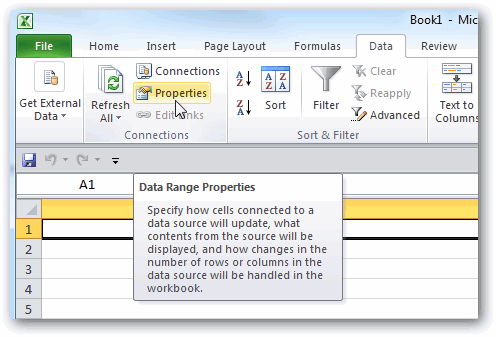
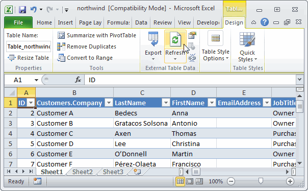
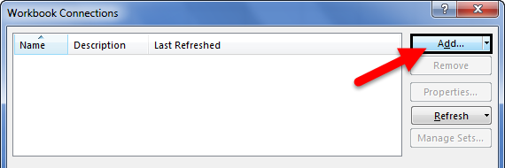
- First, we must go to the DATA tab. Then, under the DATA tab, click on Connections.

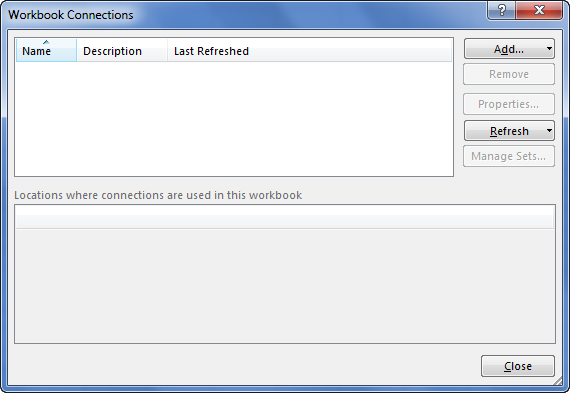
- As soon as we click on Connections, we may see the below window separately.

- Now, click on Add.

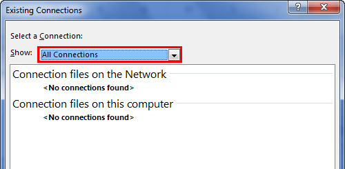
- It will open up a new window. In the below window, select All Connections.

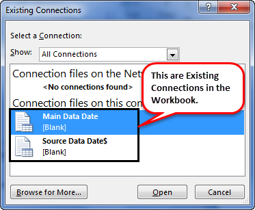
- If there are any connections in this workbook, it will show what those connections are here.

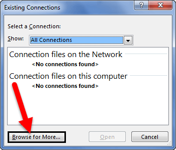
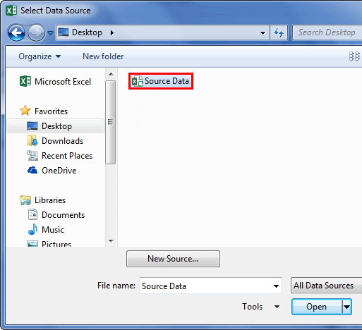
- Since we are connecting to a new workbook, click on Browse for more.

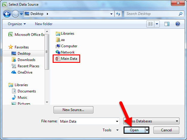
- In the below window, browse the file location. Then, click on Open.

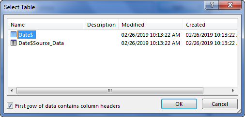
- After clicking on Open, it shows the below window.

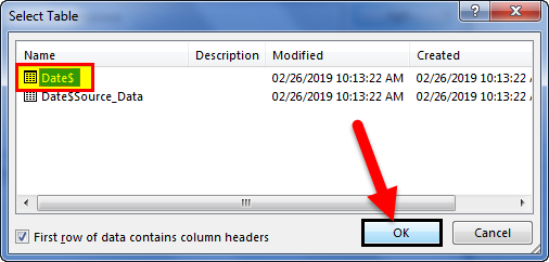
- Here, we need to select the required table to be imported to this workbook. Select the table and click on OK.
After clicking on OK, close the Workbook Connection window.
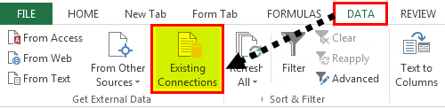
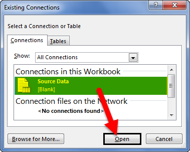
- Then, go to Existing Connections under the DATA tab.

- Here, we will see all the existing connections. Select the connection we have just made and click on Open.

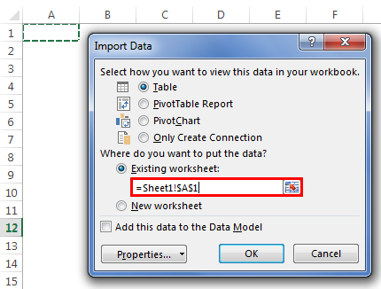
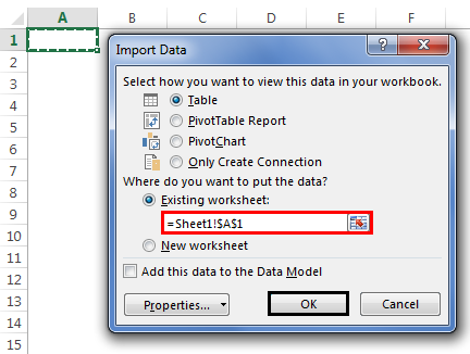
- Once we click on Open, it will ask us where to import the data. First, we need to select the cell reference here. Then, click on the OK button.

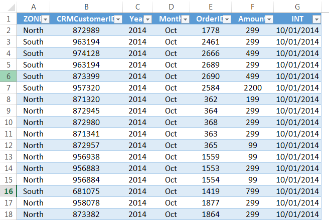
- It will import the data from the selected or connected workbook.

Like this, we can connect to the other workbook and import the data.
#2 – Import Data from MS Access to Excel
MS Access is the main platform to store the data safely. We can import the data directly from the MS Access File itself whenever the data is required.
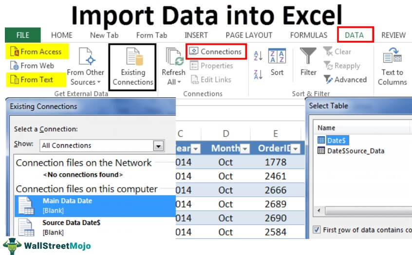
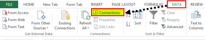
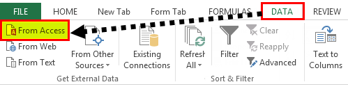
Step 1: Go to the “DATA” ribbon in excelThe ribbon is an element of the UI (User Interface) which is seen as a strip that consists of buttons or tabs; it is available at the top of the excel sheet. This option was first introduced in the Microsoft Excel 2007.read more and select “From Access.“
Step 2: Now, it will ask us to locate the desired file. Select the desired file path. Then, click on “Open.”
Step 3: Now, it will ask us to select the desired destination cell where we want to import the data. Then, click on “OK.”
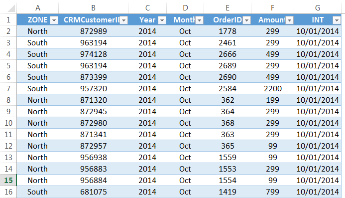
Step 4: It will import the data from access to the A1 cell in Excel.
#3 – Import Data from Text File to Excel
In almost all the corporations, whenever we ask for the data from the IT team, they will write a query and get the file in TEXT format. But unfortunately, TEXT file data is not the ready format to use in Excel; we need to make some modifications to work on it.
Step 1: Go to the “DATA” tab and click on “From Text.”

Step 2: Now, it will ask us to choose the file location on the computer or laptop. Select the targeted file, then click on “Import.”
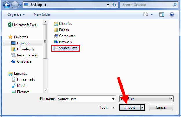
Step 3: It will open up a “Text Import Wizard.”
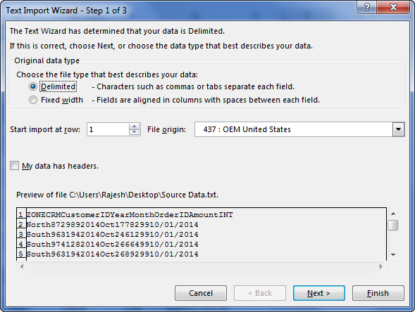
Step 4: By selecting the “Delimited,” click on “Next.”
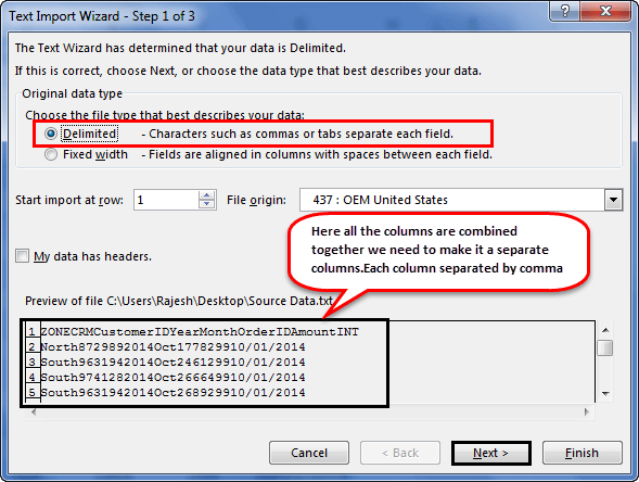
Step 5: In the next window, select the other and mention comma (,) because, in the text file, each column is separated by a comma (,). Then click on “Next.”
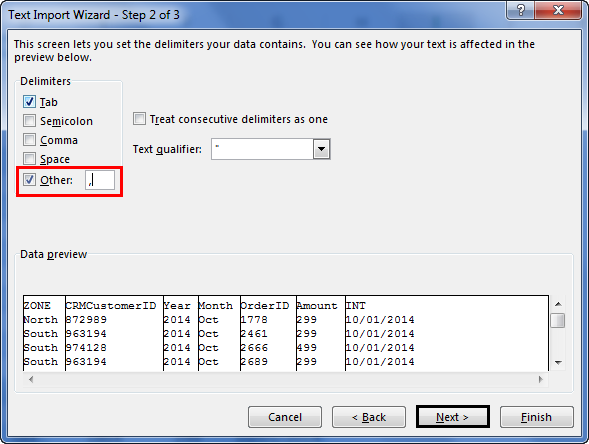
Step 6: In the next window, click on “Finish.”
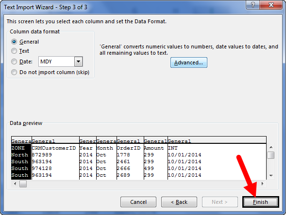
Step 7: Now, it will ask us to select the desired destination cell where we want to import the data. Select the cell and click on “OK.”
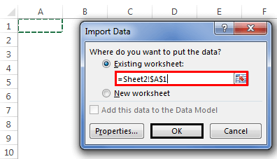
Step 8: It will import the data from the text file to the A1 cell in Excel.
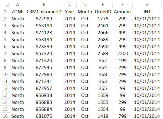
Things to Remember
- If there are many tables, we must specify which table data we need to import.
- If we want the data in the current worksheet, we need to select the desired cell. Else, if we need data in a new worksheet, we must choose the new worksheet as the option.
- We need to separate the column in the TEXT file by identifying the common column separators.
Recommended Articles
This article is a guide to Import Data in Excel. Here, we discuss how to import data from 1) Excel Workbook, 2) MS Access, 3) Text File, practical examples, and a downloadable Excel template. You may learn more about Excel from the following articles: –
- KPI Dashboard in Excel
- Insert Image in Excel Cell
- How to Insert New Worksheet In Excel?
- Create a Dashboard in Excel
- Page Numbers in Excel
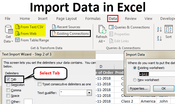
Excel Import Data (Table of Contents)
- Import Data In Excel
- How To Import Data In Excel?
Import Data In Excel
Microsoft has provided some functions that can be used to import the data from different sources and connect them with excel. We can import the data from different sources such as from Access, Web, Text, SQL Server or any other database. We can connect Microsoft Excel with many sources and import the data in many ways.
How To Import Data In Excel?
Let’s see how to import data in Excel by using some examples:
You can download this Import Data in Excel Template here – Import Data in Excel Template
Import Data In Excel – Example #1
Many times we faced a situation where we need to extract or import the data from other sources. And in Excel, we can use the function Get External Data to import the required fields to work from different sources.
We can extract the data in excel by going in the Data menu tab, under getting and Transform data, select any required source as shown below.
Those options are shown in the below screenshot.
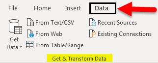
There are many different ways to import data in excel.
- From Text/CSV: Text files whose data can be separated with a tab or excel columns.
- From Web: Any website whose data can be converted to excel tables.
- From Table/Range: Create a new query linked to the selected Excel table or named range.
Above mentioned ways of importing the data are majorly used. There are some other ways also, as shown in the below screenshot. For that, click on From SQL Server Database under From Database section. Once we do that, we will get a drop-down list of all the other sources from where we can import the data.
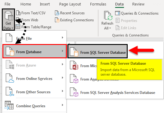
Once we import the data from any server or database, the connection gets established permanently till we remove it manually. And in the future, we can import the data from previously established and connected sources to save time. For this, go to the Data menu tab; under Get & Transform Data, select Existing Connections as shown below.
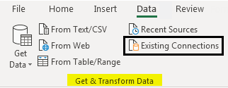
Once we click on it, we will get a list of all existing connections which we link with our computer or excel or network, as shown below. From that list, select the required connection point and click on Open to access that database.
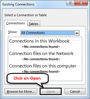
Now let’s import some data from any website. For that, we must have the link to that website from where we need to import the data. Here, for example, we have considered the link of Wikipedia as given below.
Link: https://en.wikipedia.org/wiki/Fortune_India_500
Now, go to the Data menu; under Get & Transform Data section, select From Web as shown below.
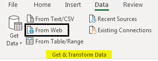
Once we do that, we will get a Web Query box. There at the address tab, copy and paste the link and click on Go as shown below.
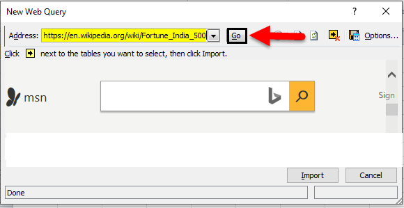
It will then take us to the web page of that link, as shown below. Now click on the Import button to import the data.
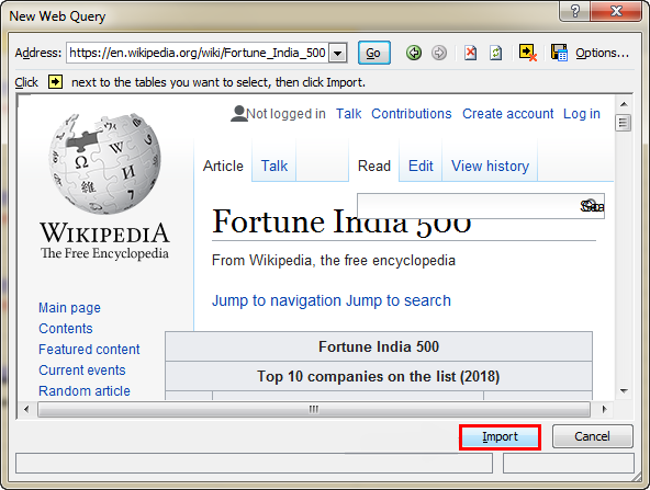
The Import Data box will appear, asking for a reference cell or sheet to import the data. Here we have select cell A1 as shown below. And click on, OK.
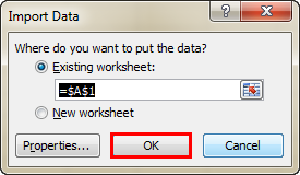
Then the query will run, and it will fetch the data from the provided link as shown below.
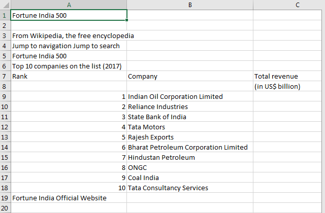
Import Data In Excel – Example #2
Let’s see another way of importing the data. For this, we have some sample data in Notepad (or Text) file, as shown below. As we can see, the data has spaces between the lines like columns in excel has.
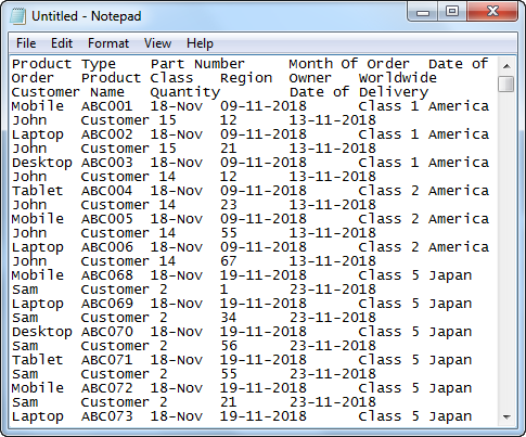
Importing such data is easy as it is already separated with spaces. Now to import the data in the text file, go to the Data menu tab, under the getting and Transform data section, select From Text option as shown below.
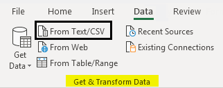
After that, we will get a box where it will ask us to browse the file. Search and select the file and click on the Import button to process further.
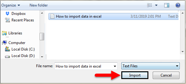
Just after that, a text import wizard will appear, which will ask us to delimit or separate the text. Select the Delimited option for a proper way to separate the data into columns or select the Fixed Width option to do it manually. Here we have selected Delimited as shown below.
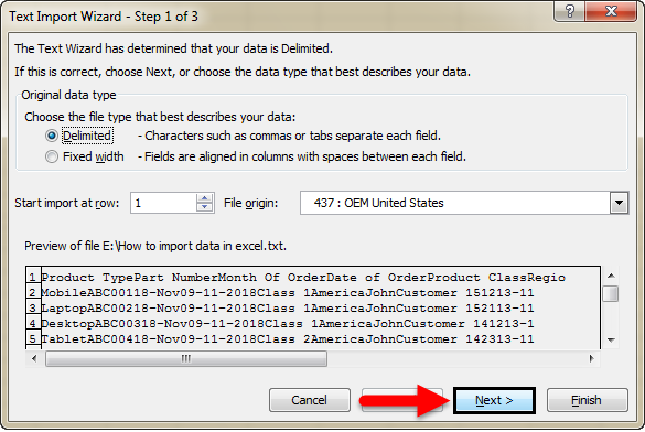
Here we have delimited the text with Tab as shown below. Now click on Next to complete the process.
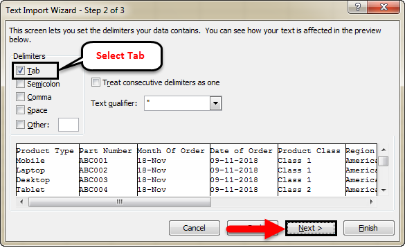
Now select the way we want to import the data. Here we have selected cell A1 for the reference point and click on OK.
We will see our data imported to excel from the selected file.
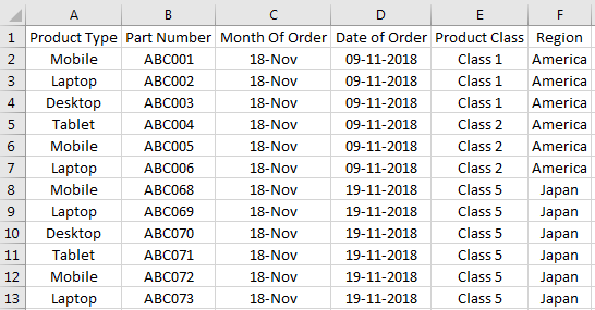
Like this, we can import the data from different sources or databases to excel to work on them.
Pros of Importing Data in Excel
- By importing the data from any other sources, we can link different tables, files, columns, or sections and get the data we require.
- It saves time by manually copying and pasting the heavy data from one source to excel.
- We also avoid unnecessary crashing or handing of files if the data is huge.
Cons of Importing Data in Excel
- Sometimes processing time is huge.
Things to Remember
- Make sure you are connected to a good internet connection when you are importing data from SQL Servers or similar databases.
- Do not do anything while data is being imported from the source files or database. It may crash the opened files.
- Always protect the previously established connection with a password.
Recommended Articles
This has been a guide to Importing Data in Excel. Here we discussed how to import data in excel along with practical examples and a downloadable excel template. You can also go through our other suggested articles to learn more –
- Auto Numbering in excel
- Watermark in Excel
- Enable Macros in excel
- Excel Uppercase Function
Возможно, вам придется использовать данные из различных источников для анализа. В Excel вы можете импортировать данные из разных источников данных. Некоторые из источников данных следующие:
- База данных Microsoft Access
- Страница интернета
- Текстовый файл
- Таблица SQL Server
- SQL Server Analysis Cube
- XML-файл
Вы можете импортировать любое количество таблиц одновременно из базы данных.
Импорт данных из базы данных Microsoft Access
Мы научимся импортировать данные из базы данных MS Access. Следуйте инструкциям ниже
Шаг 1 – Откройте новую пустую книгу в Excel.
Шаг 2 – Перейдите на вкладку ДАННЫЕ на ленте.
Шаг 3 – Нажмите « Доступ» в группе «Получить внешние данные». Откроется диалоговое окно « Выбор источника данных ».
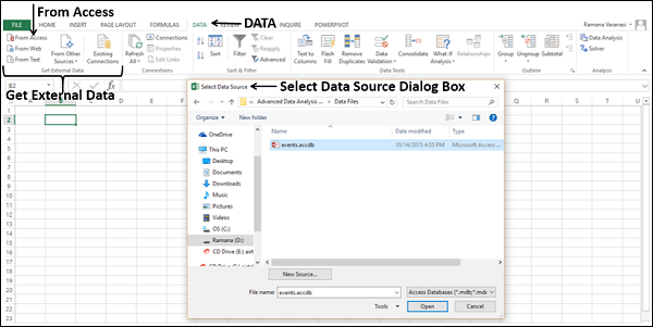
Шаг 4 – Выберите файл базы данных Access, который вы хотите импортировать. Файлы базы данных Access будут иметь расширение .accdb.
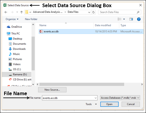
Откроется диалоговое окно «Выбор таблицы», в котором отображаются таблицы, найденные в базе данных Access. Вы можете импортировать все таблицы в базе данных одновременно или импортировать только выбранные таблицы на основе ваших потребностей анализа данных.
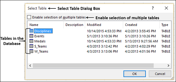
Шаг 5 – Установите флажок Включить выбор нескольких таблиц и выберите все таблицы.
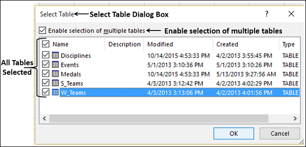
Шаг 6 – Нажмите ОК. Откроется диалоговое окно « Импорт данных ».
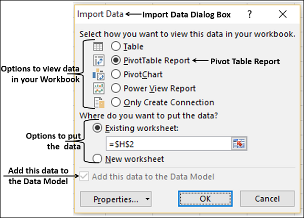
Как вы заметили, у вас есть следующие опции для просмотра данных, которые вы импортируете в свою рабочую книгу:
- Таблица
- Отчет сводной таблицы
- PivotChart
- Power View Report
У вас также есть возможность – только создать соединение . Далее отчет по сводной таблице выбран по умолчанию.
Excel также дает вам возможность поместить данные в вашу книгу –
- Существующий лист
- Новый лист
Вы найдете еще один флажок, который установлен и отключен. Добавьте эти данные в модель данных . Каждый раз, когда вы импортируете таблицы данных в свою книгу, они автоматически добавляются в модель данных в вашей книге. Вы узнаете больше о модели данных в следующих главах.
Вы можете попробовать каждый из вариантов, чтобы просмотреть импортируемые данные и проверить, как эти данные отображаются в вашей рабочей книге.
-
Если вы выберете « Таблица» , опция «Существующая рабочая таблица» будет отключена, будет выбрана опция « Новая рабочая таблица», и Excel создаст столько таблиц, сколько будет импортировано таблиц из базы данных. Таблицы Excel отображаются в этих таблицах.
-
Если вы выберете Отчет сводной таблицы , Excel импортирует таблицы в рабочую книгу и создаст пустую сводную таблицу для анализа данных в импортированных таблицах. У вас есть возможность создать сводную таблицу на существующем листе или новом листе.
Таблицы Excel для импортированных таблиц данных не будут отображаться в книге. Однако вы найдете все таблицы данных в списке полей сводной таблицы вместе с полями в каждой таблице.
-
Если вы выберете PivotChart , Excel импортирует таблицы в рабочую книгу и создаст пустую PivotChart для отображения данных в импортированных таблицах. У вас есть возможность создать сводную диаграмму на существующем или новом листе.
Таблицы Excel для импортированных таблиц данных не будут отображаться в книге. Однако вы найдете все таблицы данных в списке полей PivotChart вместе с полями в каждой таблице.
-
Если вы выберите Power View Report , Excel импортирует таблицы в рабочую книгу и создаст Power View Report в новой рабочей таблице. В последующих главах вы узнаете, как использовать отчеты Power View для анализа данных.
Таблицы Excel для импортированных таблиц данных не будут отображаться в книге. Однако вы найдете все таблицы данных в списке полей Power View Report вместе с полями в каждой таблице.
-
Если вы выберете опцию – Только создать соединение , между базой данных и вашей книгой будет установлено соединение для передачи данных. Таблицы или отчеты не отображаются в книге. Однако импортированные таблицы по умолчанию добавляются в модель данных в вашей книге.
Вам необходимо выбрать любой из этих параметров в зависимости от вашего намерения импортировать данные для анализа данных. Как вы заметили выше, независимо от выбранной вами опции, данные импортируются и добавляются в модель данных в вашей рабочей книге.
Если вы выберете « Таблица» , опция «Существующая рабочая таблица» будет отключена, будет выбрана опция « Новая рабочая таблица», и Excel создаст столько таблиц, сколько будет импортировано таблиц из базы данных. Таблицы Excel отображаются в этих таблицах.
Если вы выберете Отчет сводной таблицы , Excel импортирует таблицы в рабочую книгу и создаст пустую сводную таблицу для анализа данных в импортированных таблицах. У вас есть возможность создать сводную таблицу на существующем листе или новом листе.
Таблицы Excel для импортированных таблиц данных не будут отображаться в книге. Однако вы найдете все таблицы данных в списке полей сводной таблицы вместе с полями в каждой таблице.
Если вы выберете PivotChart , Excel импортирует таблицы в рабочую книгу и создаст пустую PivotChart для отображения данных в импортированных таблицах. У вас есть возможность создать сводную диаграмму на существующем или новом листе.
Таблицы Excel для импортированных таблиц данных не будут отображаться в книге. Однако вы найдете все таблицы данных в списке полей PivotChart вместе с полями в каждой таблице.
Если вы выберите Power View Report , Excel импортирует таблицы в рабочую книгу и создаст Power View Report в новой рабочей таблице. В последующих главах вы узнаете, как использовать отчеты Power View для анализа данных.
Таблицы Excel для импортированных таблиц данных не будут отображаться в книге. Однако вы найдете все таблицы данных в списке полей Power View Report вместе с полями в каждой таблице.
Если вы выберете опцию – Только создать соединение , между базой данных и вашей книгой будет установлено соединение для передачи данных. Таблицы или отчеты не отображаются в книге. Однако импортированные таблицы по умолчанию добавляются в модель данных в вашей книге.
Вам необходимо выбрать любой из этих параметров в зависимости от вашего намерения импортировать данные для анализа данных. Как вы заметили выше, независимо от выбранной вами опции, данные импортируются и добавляются в модель данных в вашей рабочей книге.
Импорт данных с веб-страницы
Иногда вам может понадобиться использовать данные, которые обновляются на веб-сайте. Вы можете импортировать данные из таблицы на веб-сайте в Excel.
Шаг 1 – Откройте новую пустую книгу в Excel.
Шаг 2 – Перейдите на вкладку ДАННЫЕ на ленте.
Шаг 3 – Нажмите « Из Интернета» в группе « Получить внешние данные ». Откроется диалоговое окно « Новый веб-запрос ».
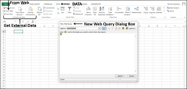
Шаг 4 – Введите URL-адрес веб-сайта, с которого вы хотите импортировать данные, в поле рядом с адресом и нажмите «Перейти».
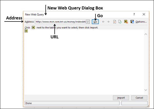
Шаг 5 – Данные на сайте появляются. Рядом с данными таблицы будут отображаться желтые значки со стрелками, которые можно импортировать.
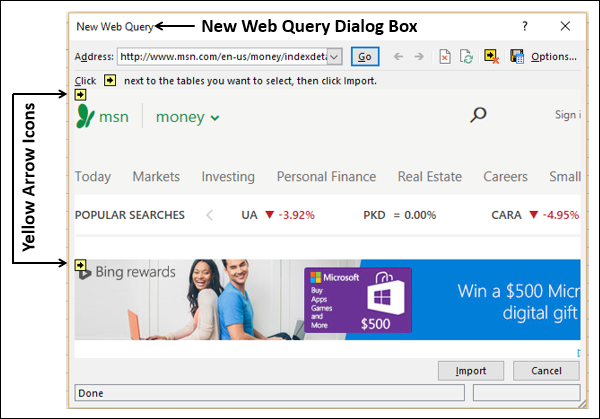
Шаг 6 – Нажмите желтые значки, чтобы выбрать данные, которые вы хотите импортировать. Это превращает желтые значки в зеленые поля с галочкой, как показано на следующем снимке экрана.
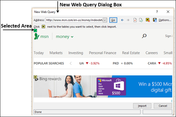
Шаг 7 – Нажмите кнопку «Импорт» после того, как вы выбрали то, что вы хотите.
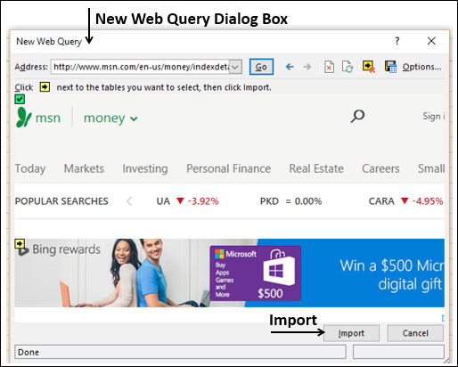
Откроется диалоговое окно « Импорт данных ».
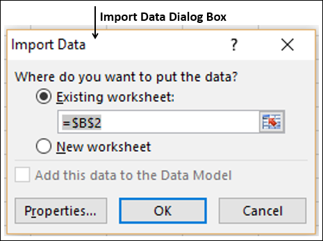
Шаг 8 – Укажите, куда вы хотите поместить данные и нажмите Ok.
Шаг 9 – Организовать данные для дальнейшего анализа и / или представления.
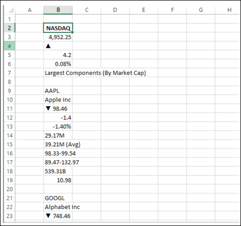
Копировать-вставить данные из Интернета
Другой способ получения данных с веб-страницы – копирование и вставка необходимых данных.
Шаг 1 – Вставьте новый лист.
Шаг 2 – Скопируйте данные с веб-страницы и вставьте их на лист.
Шаг 3 – Создайте таблицу с вставленными данными.
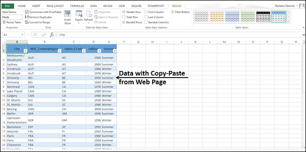
Импорт данных из текстового файла
Если у вас есть данные в файлах .txt или .csv или .prn , вы можете импортировать данные из этих файлов, рассматривая их как текстовые файлы. Следуйте инструкциям ниже
Шаг 1 – Откройте новый лист в Excel.
Шаг 2 – Перейдите на вкладку ДАННЫЕ на ленте.
Шаг 3 – Нажмите « Из текста» в группе «Получить внешние данные». Откроется диалоговое окно « Импорт текстового файла ».
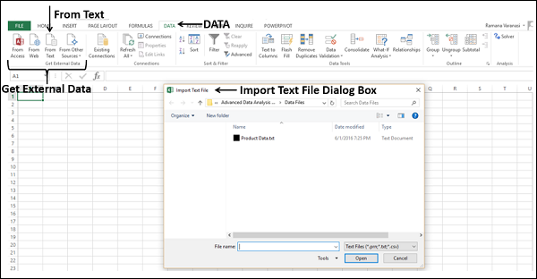
Вы можете видеть, что текстовые файлы с расширениями .prn, .txt и .csv принимаются.
Шаг 4 – Выберите файл. Имя выбранного файла появится в поле Имя файла. Кнопка «Открыть» изменится на кнопку «Импорт».
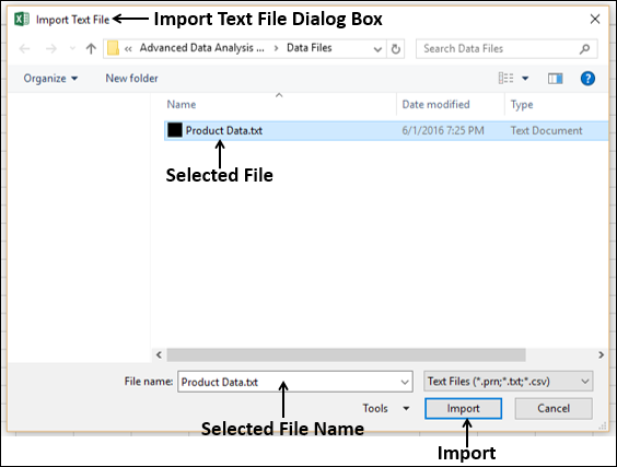
Шаг 5 – Нажмите кнопку «Импорт». Мастер импорта текста – появляется диалоговое окно « Шаг 1 из 3 ».
Шаг 6 – Выберите опцию «С разделителями», чтобы выбрать тип файла, и нажмите «Далее».
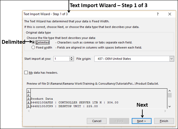
Откроется мастер импорта текста – шаг 2 из 3 .
Шаг 7 – В разделе «Разделители» выберите « Другое» .
Шаг 8 – В поле рядом с Другой введите | (Это разделитель в текстовом файле, который вы импортируете).
Шаг 9 – Нажмите Далее.
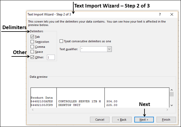
Откроется мастер импорта текста – шаг 3 из 3 .
Шаг 10 – В этом диалоговом окне вы можете установить формат данных столбца для каждого из столбцов.
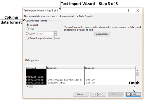
Шаг 11. После завершения форматирования данных столбцов нажмите кнопку «Готово». Откроется диалоговое окно « Импорт данных ».
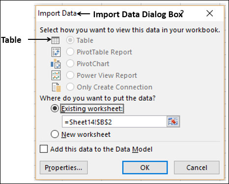
Вы увидите следующее –
-
Таблица выбрана для просмотра и отображается серым цветом. Таблица – единственный вариант просмотра, который у вас есть в этом случае.
-
Вы можете поместить данные либо в существующий рабочий лист, либо в новый рабочий лист.
-
Вы можете установить или не устанавливать флажок Добавить эти данные в модель данных.
-
Нажмите OK после того, как вы сделали выбор.
Таблица выбрана для просмотра и отображается серым цветом. Таблица – единственный вариант просмотра, который у вас есть в этом случае.
Вы можете поместить данные либо в существующий рабочий лист, либо в новый рабочий лист.
Вы можете установить или не устанавливать флажок Добавить эти данные в модель данных.
Нажмите OK после того, как вы сделали выбор.
Данные появятся на указанном вами листе. Вы импортировали данные из текстового файла в книгу Excel.
Импорт данных из другой книги
Возможно, вам придется использовать данные из другой книги Excel для анализа данных, но кто-то другой может поддерживать другую книгу.
Чтобы получать последние данные из другой книги, установите соединение данных с этой книгой.
Шаг 1 – Нажмите DATA> Соединения в группе Соединения на ленте.
Откроется диалоговое окно « Подключения к книге».
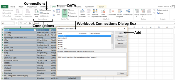
Шаг 2. Нажмите кнопку «Добавить» в диалоговом окне «Подключения к книге». Откроется диалоговое окно « Существующие подключения ».
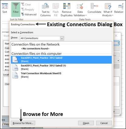
Шаг 3 – Нажмите кнопку Обзор для более … Откроется диалоговое окно « Выбор источника данных ».
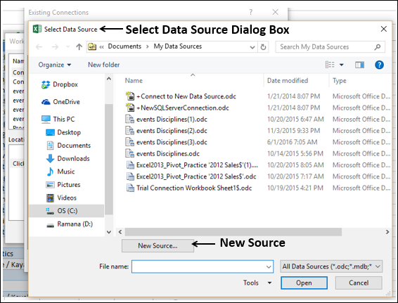
Шаг 4 – Нажмите кнопку « Новый источник» . Откроется диалоговое окно мастера подключения к данным .
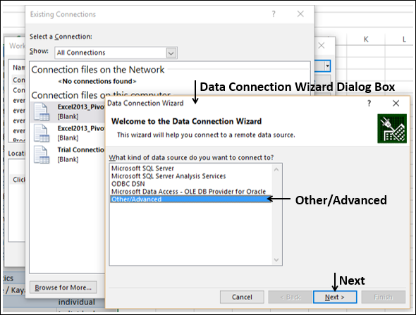
Шаг 5 – Выберите Other / Advanced в списке источников данных и нажмите Next. Откроется диалоговое окно «Свойства ссылки на данные».
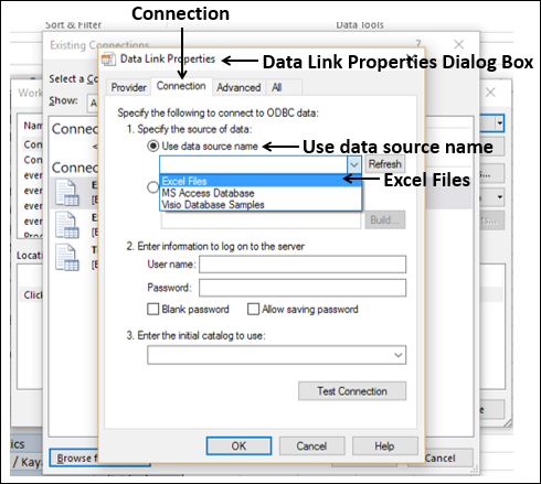
Шаг 6 – Установите свойства канала передачи данных следующим образом –
-
Перейдите на вкладку « Соединение ».
-
Нажмите Использовать имя источника данных.
-
Нажмите стрелку вниз и выберите « Файлы Excel» в раскрывающемся списке.
-
Нажмите ОК.
Перейдите на вкладку « Соединение ».
Нажмите Использовать имя источника данных.
Нажмите стрелку вниз и выберите « Файлы Excel» в раскрывающемся списке.
Нажмите ОК.
Откроется диалоговое окно « Выбрать рабочую книгу ».
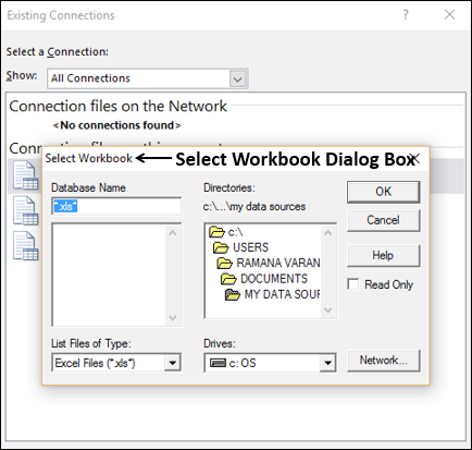
Шаг 7 – Найдите место, где у вас есть рабочая книга для импорта. Нажмите ОК.
Откроется диалоговое окно « Мастер подключения к данным » с выбором базы данных и таблицы.
Примечание. В этом случае Excel обрабатывает каждый рабочий лист, который импортируется, как таблицу. Имя таблицы будет именем рабочего листа. Таким образом, чтобы иметь значимые имена таблиц, назовите / переименуйте рабочие листы в зависимости от ситуации.
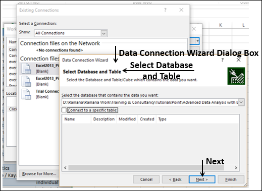
Шаг 8 – Нажмите Далее. Откроется диалоговое окно мастера подключения к данным с сохранением файла подключения к данным и завершением.
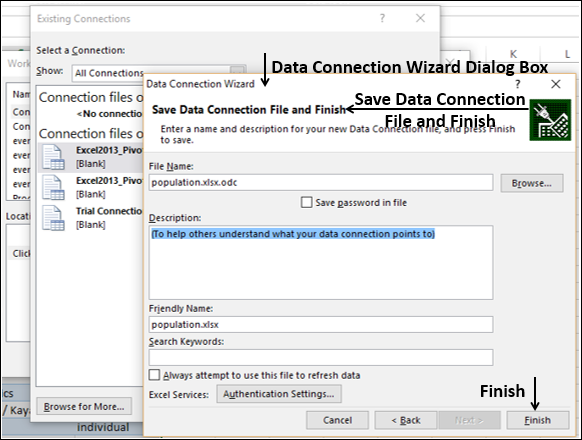
Шаг 9 – Нажмите кнопку Готово. Откроется диалоговое окно « Выбор таблицы ».
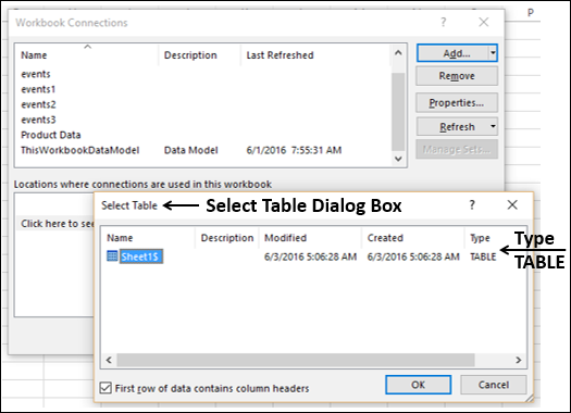
Как вы заметили, Name – это имя листа, которое импортируется как тип TABLE. Нажмите ОК.
Соединение данных с выбранной вами рабочей книгой будет установлено.
Импорт данных из других источников
Excel предоставляет вам возможность выбора различных других источников данных. Вы можете импортировать данные из них в несколько шагов.
Шаг 1 – Откройте новую пустую книгу в Excel.
Шаг 2 – Перейдите на вкладку ДАННЫЕ на ленте.
Шаг 3 – Нажмите Из других источников в группе Получить внешние данные.
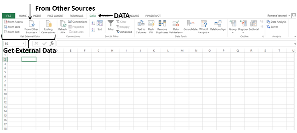
Появляется выпадающий список с различными источниками данных.
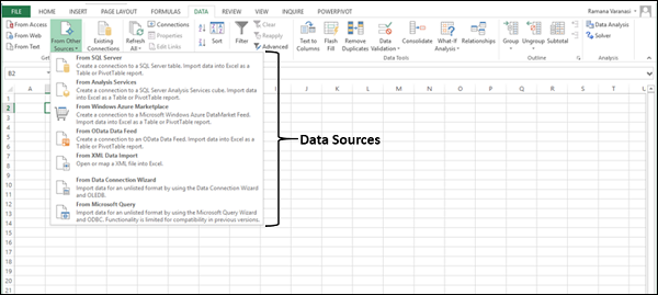
Вы можете импортировать данные из любого из этих источников данных в Excel.
Импорт данных с использованием существующего соединения
В предыдущем разделе вы установили соединение для передачи данных с книгой.
Теперь вы можете импортировать данные, используя это существующее соединение.
Шаг 1 – Перейдите на вкладку ДАННЫЕ на ленте.
Шаг 2 – Нажмите Существующие соединения в группе Получить внешние данные. Откроется диалоговое окно «Существующие подключения».
Шаг 3 – Выберите соединение, из которого вы хотите импортировать данные, и нажмите «Открыть».
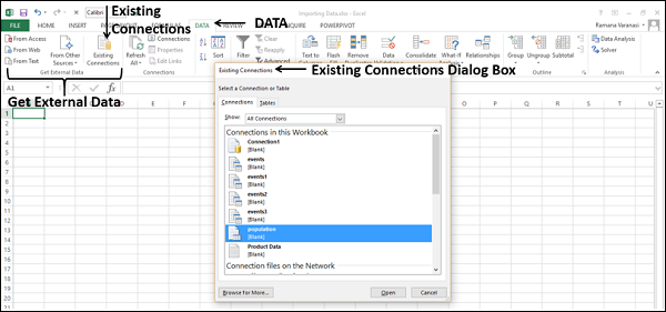
Переименование соединений данных
Будет полезно, если у подключений к данным, которые есть в вашей книге, есть понятные имена для простоты понимания и определения местоположения.
Шаг 1 – Перейдите в DATA> Соединения на ленте. Откроется диалоговое окно « Подключения к книге».
Шаг 2 – Выберите соединение, которое вы хотите переименовать, и нажмите Свойства.
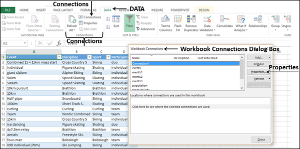
Откроется диалоговое окно « Свойства соединения ». Текущее имя появится в поле Имя соединения –
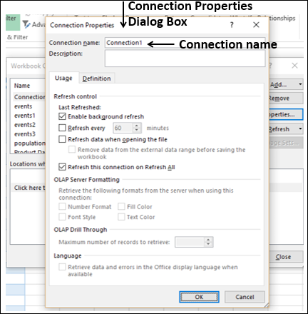
Шаг 3 – Измените имя соединения и нажмите ОК. Передача данных будет иметь новое имя, которое вы дали.
Обновление подключения к внешним данным
Когда вы подключаете свою книгу Excel к внешнему источнику данных, как вы видели в предыдущих разделах, вы хотели бы регулярно обновлять данные в своей книге, отражая изменения, вносимые во внешний источник данных время от времени.
Вы можете сделать это, обновив соединения данных, которые вы сделали с этими источниками данных. Всякий раз, когда вы обновляете соединение данных, вы видите самые последние изменения данных из этого источника данных, включая все, что является новым, или которое было изменено, или которое было удалено.
Вы можете обновить только выбранные данные или все подключения данных в книге одновременно.
Шаг 1 – Перейдите на вкладку ДАННЫЕ на ленте.
Шаг 2 – Нажмите « Обновить все» в группе «Подключения».
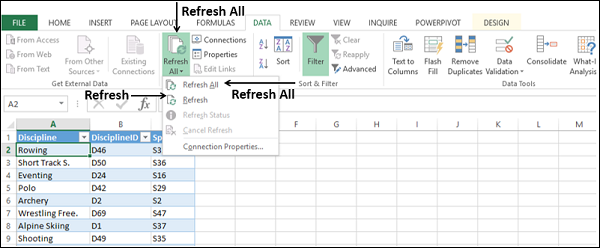
Как вы заметили, в выпадающем списке есть две команды – Обновить и Обновить все.
-
Если вы нажмете Обновить , выбранные данные в вашей рабочей книге будут обновлены.
-
Если вы нажмете Обновить все , все подключения к данным в вашей книге будут обновлены.
Если вы нажмете Обновить , выбранные данные в вашей рабочей книге будут обновлены.
Если вы нажмете Обновить все , все подключения к данным в вашей книге будут обновлены.
Обновление всех соединений данных в рабочей книге
У вас может быть несколько подключений к вашей книге. Вам необходимо время от времени обновлять их, чтобы ваша рабочая книга имела доступ к самым последним данным.
Шаг 1 – Нажмите любую ячейку в таблице, которая содержит ссылку на импортированный файл данных.
Шаг 2 – Перейдите на вкладку «Данные» на ленте.
Шаг 3 – Нажмите «Обновить все» в группе «Подключения».
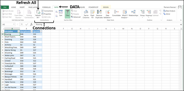
Шаг 4 – Выберите Обновить все из выпадающего списка. Все подключения к данным в рабочей книге будут обновлены.
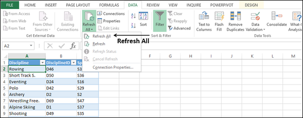
Автоматически обновлять данные при открытии рабочей книги
Возможно, вы захотите иметь доступ к последним данным из подключений к вашей книге при каждом открытии вашей книги.
Шаг 1 – Нажмите любую ячейку в таблице, которая содержит ссылку на импортированный файл данных.
Шаг 2 – Перейдите на вкладку «Данные».
Шаг 3 – Нажмите «Подключения» в группе «Подключения».
Откроется диалоговое окно «Подключения к книге».
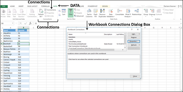
Шаг 4 – Нажмите кнопку Свойства. Откроется диалоговое окно «Свойства соединения».
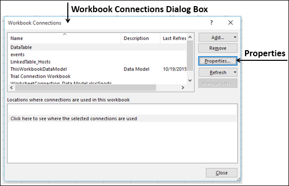
Шаг 5 – Перейдите на вкладку «Использование».
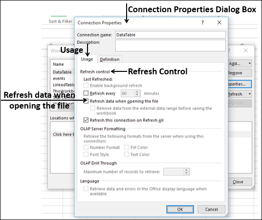
Шаг 6 – Отметьте опцию – Обновить данные при открытии файла.
У вас есть и другой вариант – удалить данные из диапазона внешних данных перед сохранением книги . Вы можете использовать эту опцию, чтобы сохранить книгу с определением запроса, но без внешних данных.
Шаг 7 – Нажмите ОК. Всякий раз, когда вы открываете свою рабочую книгу, в вашу рабочую книгу загружаются самые свежие данные.
Автоматически обновлять данные через регулярные интервалы
Возможно, вы используете свою рабочую книгу, чтобы держать ее открытой в течение более длительного времени. В таком случае вы можете периодически обновлять данные без какого-либо вмешательства с вашей стороны.
Шаг 1 – Нажмите любую ячейку в таблице, которая содержит ссылку на импортированный файл данных.
Шаг 2 – Перейдите на вкладку «Данные» на ленте.
Шаг 3 – Нажмите «Подключения» в группе «Подключения».
Откроется диалоговое окно «Подключения к книге».
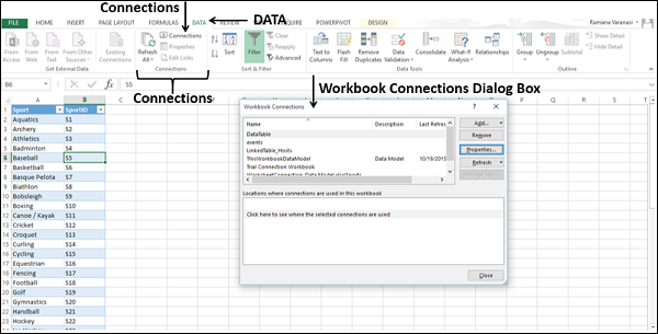
Шаг 4 – Нажмите кнопку Свойства.

Откроется диалоговое окно «Свойства соединения». Установите свойства следующим образом –
-
Перейдите на вкладку « Использование ».
-
Установите флажок Обновить каждый .
-
Введите 60 в качестве количества минут между каждой операцией обновления и нажмите Ok.
Перейдите на вкладку « Использование ».
Установите флажок Обновить каждый .
Введите 60 в качестве количества минут между каждой операцией обновления и нажмите Ok.
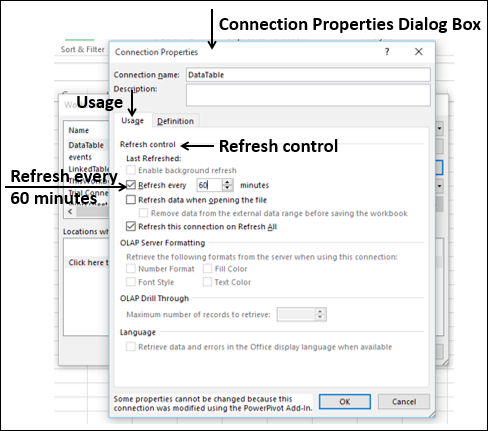
Ваши данные будут автоматически обновляться каждые 60 минут. (т.е. каждый час).
Включение фонового обновления
Для очень больших наборов данных рекомендуется запустить фоновое обновление. Это возвращает управление Excel вместо того, чтобы заставлять вас ждать несколько минут или более, пока обновление не закончится. Вы можете использовать эту опцию, когда вы выполняете запрос в фоновом режиме. Однако в течение этого времени нельзя выполнить запрос для любого типа соединения, который извлекает данные для модели данных.
-
Щелкните в любой ячейке таблицы, содержащей ссылку на импортированный файл данных.
-
Перейдите на вкладку «Данные».
-
Нажмите Подключения в группе Подключения. Откроется диалоговое окно «Подключения к книге».
Щелкните в любой ячейке таблицы, содержащей ссылку на импортированный файл данных.
Перейдите на вкладку «Данные».
Нажмите Подключения в группе Подключения. Откроется диалоговое окно «Подключения к книге».
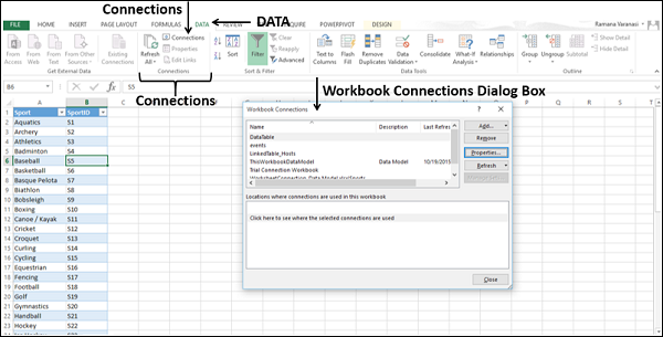
Нажмите кнопку Свойства.

Откроется диалоговое окно «Свойства соединения». Перейдите на вкладку «Использование». Появятся параметры управления обновлением.
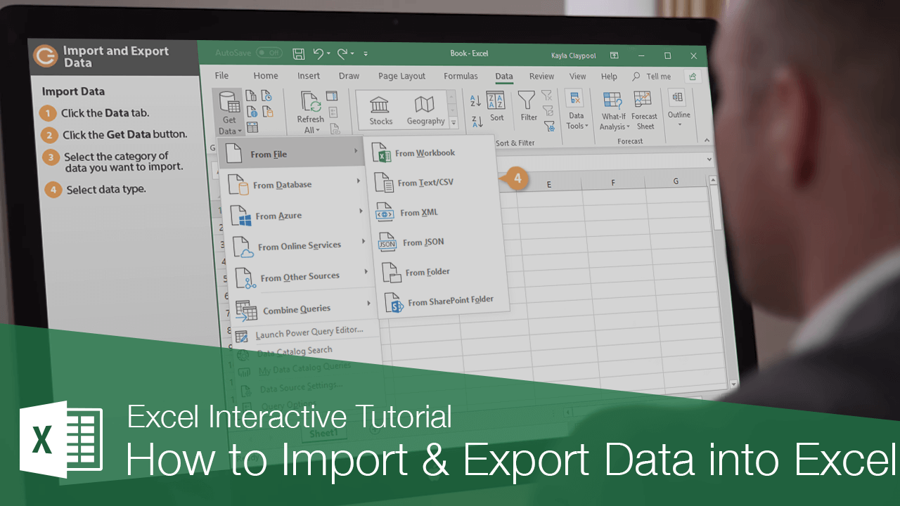
Excel can import and export many different file types aside from the standard .xslx format. If your data is shared between other programs, like a database, you may need to save data as a different file type or bring in files of a different file type.
Export Data
When you have data that needs to be transferred to another system, export it from Excel in a format that can be interpreted by other programs, such as a text or CSV file.
- Click the File tab.

- At the left, click Export.
- Click the Change File Type.
- Under Other File Types, select a file type.
- Text (Tab delimited): The cell data will be separated by a tab.
- CSV (Comma delimited): The cell data will be separated by a comma.
- Formatted Text (space delimited): The cell data will be separated by a space.
- Save as Another File Type: Select a different file type when the Save As dialog box appears.
The file type you select will depend on what type of file is required by the program that will consume the exported data.
- Click Save As.

- Specify where you want to save the file.
- Click Save.
A dialog box appears stating that some of the workbook features may be lost.
- Click Yes.
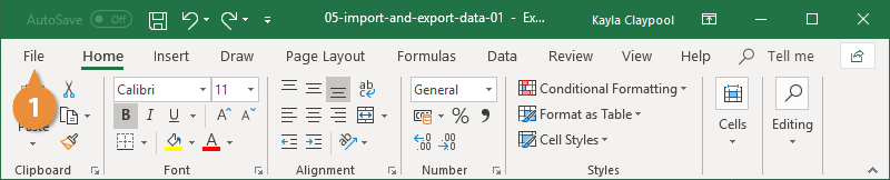
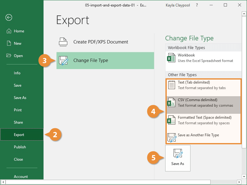
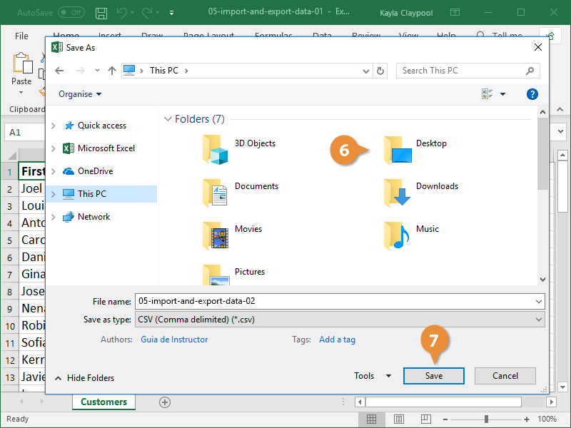
Import Data
Excel can import data from external data sources including other files, databases, or web pages.
- Click the Data tab on the Ribbon..
- Click the Get Data button.
Some data sources may require special security access, and the connection process can often be very complex. Enlist the help of your organization’s technical support staff for assistance.
- Select From File.
- Select From Text/CSV.
If you have data to import from Access, the web, or another source, select one of those options in the Get External Data group instead.
- Select the file you want to import.
- Click Import.
If, while importing external data, a security notice appears saying that it is connecting to an external source that may not be safe, click OK.
- Verify the preview looks correct.
Because we’ve specified the data is separated by commas, the delimiter is already set. If you need to change it, it can be done from this menu.
- Click Load.
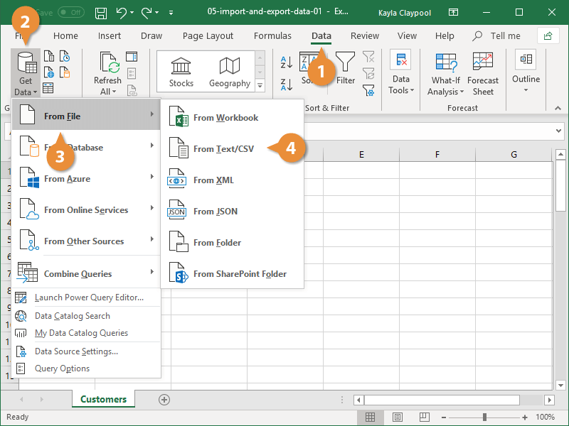
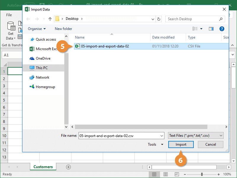
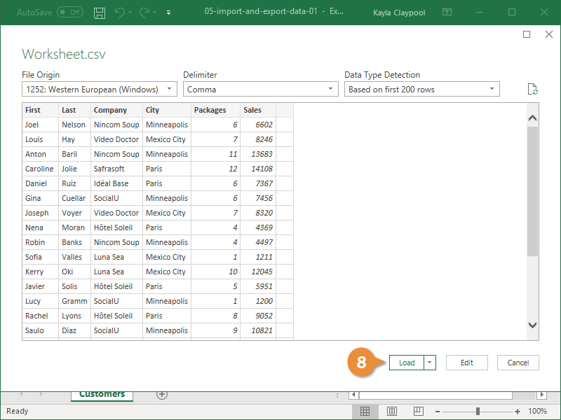

FREE Quick Reference
Click to Download
Free to distribute with our compliments; we hope you will consider our paid training.
How to Import Excel Data into a Word Table
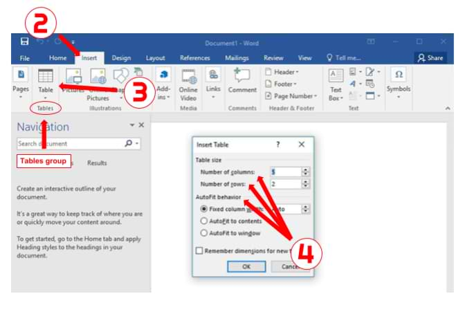
This help page will show you how to import data from Excel into a Microsoft Word table.
- Open a new or existing document in Microsoft Word.
- Click the «Insert» tab > Locate the «Tables» group.
- Select the «Table» icon > Choose the «Insert Table…» option.
- Set the «Number of columns,» «Number of rows,» and «AutoFit behavior» to your desired specifications > Click [OK].
- Open the Excel file and use your mouse to select the data you wish to import.
- Right-click on the range of cells you have highlighted and select «Copy.»
- Switch back to Word and highlight the table cells where you want to import the Excel data.
- Right-click on the Word table and click the option you want under «Paste Options.»
Note:
If you select the table in Word, the «Table Tools» tab will appear at the top of the page. Use this tab to format the «Design» and «Layout» of the table to meet your preferences.
Keywords: transfer, convert, change, Excel to Word, export, move, copy, import, Excel 2007, Word 2007, Microsoft, micro soft
Share This Post
-
Facebook
-
Twitter
-
LinkedIn
External data is defined as data that exists outside of the Excel workbook, in some other place. Other places could be almost anywhere; and Excel supports pulling external data from a wide variety of sources. Examples include data stored on web pages, in text files, or in other programs.
Excel 2007 is been used in below examples.
We get external data in excel by using different ways:-
- From Access
- From Web
- From Text
- From Other Sources
- From SQL Server
- From XML Data Import
I) Import Access Data
In Excel, when you import data, you make a permanent connection that can be refreshed.
- On the Data tab, in the Get External Data group, click From Access.

- Select the Access file.

- Click Open.
- Select a table and click OK.

- Select how you want to view this data, where you want to put it, and click OK.


Result. Your database records in Excel.

- When your Access data changes, you can easily refresh the data in Excel. First, select a cell inside the table. Next, on the Design tab, in the External Table Data group, click Refresh.


II) Import Web Data
- On the Data tab, in the Get External Data group, click From Web.

- When you select From Web Excel opens a dialog box displaying your browser homepage with the URL of the page highlighted. Paste the copied web address into the Address box. A quick way to paste is to Hold down the Ctrl Key as you tap one time on the V key( Ctrl + V ). You may have to scroll to find the data table. When you find it, click one time on the arrow next to the Data table and then click on the Import button.

- You have a choice to make. Excel is ready to import the data, but needs to know if you want it put into the existing workbook, or a new workbook.


III) Import Text Data
- On the ribbon, click the data tab and then click the “From Text” button on the “Get External data” group.

The “From Text” button, located on the Data tab of the ribbon.
- Select your file from the next dialog:


And Click Import.
- Now it is time to define what settings we need for the import.Click the Open button. The text import wizard opens up:


Step 1 of the Text Import Wizard, define file type.
In this example I have selected to import a delimited file and set the file origin to Windows (ANSI). Click Next when you’re happy with the settings.
- Step 2 of the wizard allows us to define the delimiters. I selected Comma:

Step 2 of the Text Import Wizard: define delimiters.
- Click Next again to go into the third step, where you can select a format for each column of your file. I changed the date format of the first column to dmy order. Click a column to set up its formatting.


Step 3 of the wizard, Define column formats.
You can click the advanced button to set up details like the decimal and thousands separators (note I switched them here):
The Advanced text Import Settings dialog.
Note that any changes made in this dialog apply to all columns.
- After you finished defining all columns, click the Finish button. Excel opens the Import Data dialog, asking where to put the results. Select the proper location.


The Import Data dialog.
- Import your data
Finally, click OK to have your data imported. My sheet looks like this:
Results after importing the text file.
- Refresh your data
On the Data tab, find the group called “Connections”. Click the dropdown “Refresh All” and select “Refresh”:
The Refresh All button on the ribbon.
IV) Import Data from Other Sources
- Import SQL Server Data
On the Data tab, in the Get External Data group, click From Other Sources.

- Click From SQL Server.

- In the Data Connection Wizard, enter the server name and logon credentials, and click Next.

- Choose the database and tables you want to work with, and click Next.

- You can click Finish, or click Next to change details for the connection.

- In the Import Data dialog box that appears, choose where to put the data in your workbook and whether to view the data as a table, Pivot Table report, or Pivot Chart.

- Import your data

Finally, click OK to have your data imported. My sheet looks like this:

- Import XML Data Files
On the Data tab, in the Get External Data group, click From Other Sources.
- From Other Sources > From XML Data Import.

- Go to the drive, folder, or Internet location that has the XML data file (.xml) you want to import. Select the file and click Open.

- In the Import Datadialog box, do one of the following:


-
- XML table in existing worksheet: The contents of the file are imported into a new XML table in a new worksheet. If the XML data file doesn’t refer to a schema, Excel infers the schema from the XML data file.

- XML table in existing worksheet: The contents of the file are imported into a new XML table in a new worksheet. If the XML data file doesn’t refer to a schema, Excel infers the schema from the XML data file.

-
- Existing worksheet: The XML data is imported in a two-dimensional table with rows and columns that shows XML tags as column headings, and data in rows below the column headings. The first element (the root node) is used like a title and is displayed in the specified cell location. The rest of the tags are sorted alphabetically across the second row. In this case, Excel doesn’t infer a schema, and you can’t use an XML Map.

- Existing worksheet: The XML data is imported in a two-dimensional table with rows and columns that shows XML tags as column headings, and data in rows below the column headings. The first element (the root node) is used like a title and is displayed in the specified cell location. The rest of the tags are sorted alphabetically across the second row. In this case, Excel doesn’t infer a schema, and you can’t use an XML Map.

-
- New worksheet: Excel adds a new worksheet to your workbook and automatically puts the XML data in the upper-left corner of the new worksheet. If the XML data file doesn’t refer to a schema, Excel infers the schema from the XML data file.

- Excel sheet will look like this:

References
- https://www.gcflearnfree.org/excel2007
- https://support.office.com/en-US/Excel

About Suman Maity:
Suman Maity is a B.Tech(Electrical Engineering) . Currently he is working as an Analyst Intern with NikhilGuru Consulting Analytics Service LLP, Bangalore. He has prior worked for around 1+ year with T&M Services Consulting Pvt Ltd and HR Chamber Outsourcing Pvt Ltd.