
Watch Video – How to Insert Picture into a Cell in Excel
A few days ago, I was working with a data set that included a list of companies in Excel along with their logos.
I wanted to place the logo of each company in the cell adjacent to its name and lock it in such a way that when I resize the cell, the logo should resize as well.
I also wanted the logos to get filtered when I filter the name of the companies.
Wishful Thinking? Not Really.
You can easily insert a picture into a cell in Excel in a way that when you move, resize, and/or filter the cell, the picture also moves/resizes/filters.
Below is an example where the logos of some popular companies are inserted in the adjacent column, and when the cells are filtered, the logos also get filtered with the cells.
This could also be useful if you’re working with products/SKUs and their images.
When you insert an image in Excel, it not linked to the cells and would not move, filter, hide, and resize with cells.
In this tutorial, I will show you how to:
- Insert a Picture Into a Cell in Excel.
- Lock the Picture in the cell so that it moves, resizes, and filters with the cells.
Insert Picture into a Cell in Excel
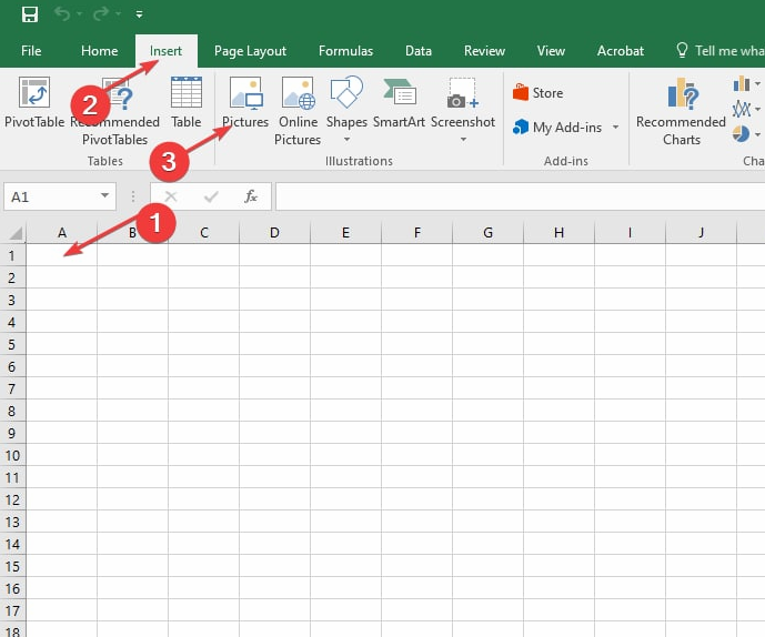
Here are the steps to insert a picture into a cell in Excel:
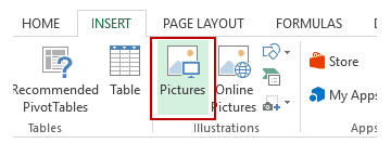
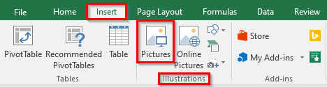
- Go to the Insert tab.
- Click on the Pictures option (it’s in the illustrations group).

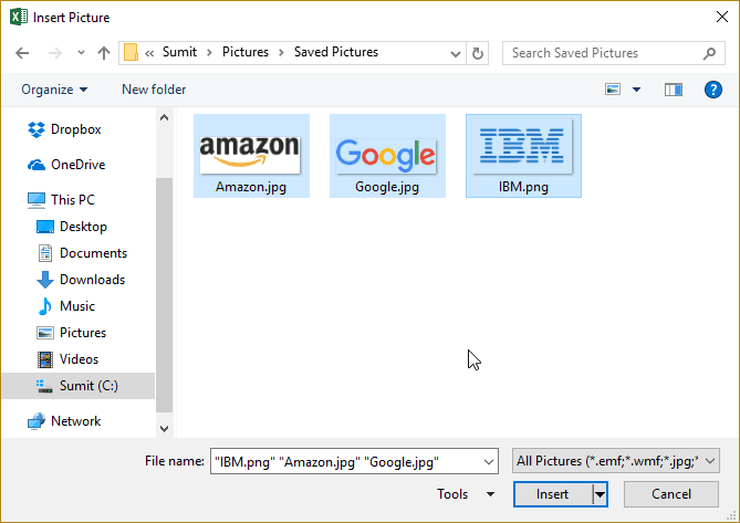
- In the ‘Insert Picture’ dialog box, locate the pictures that you want to insert into a cell in Excel.

- Click on the Insert button.
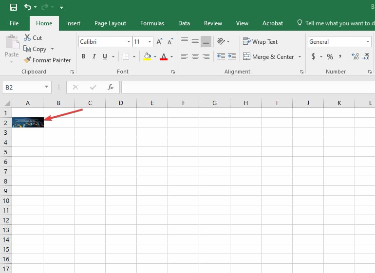
- Re-size the picture/image so that it can fit perfectly within the cell.

- Place the picture in the cell.
- A cool way to do this is to first press the ALT key and then move the picture with the mouse. It will snap and arrange itself with the border of the cell as soon it comes close to it.

- A cool way to do this is to first press the ALT key and then move the picture with the mouse. It will snap and arrange itself with the border of the cell as soon it comes close to it.


If you have multiple images, you can select and insert all the images at once (as shown in step 4).
You can also resize images by selecting it and dragging the edges. In the case of logos or product images, you may want to keep the aspect ratio of the image intact. To keep the aspect ratio intact, use the corners of an image to resize it.
When you place an image within a cell using the steps above, it will not stick with the cell in case you resize, filter, or hide the cells. If you want the image to stick to the cell, you need to lock the image to the cell it’s placed n.
To do this, you need to follow the additional steps as shown in the section below.
Lock the Picture with the Cell in Excel
Once you have inserted the image into the workbook, resized it ti fit within a cell, and placed it in the cell, you need to lock it to make sure it moves, filters, and hides with the cell.
Here are the steps to lock a picture in a cell:
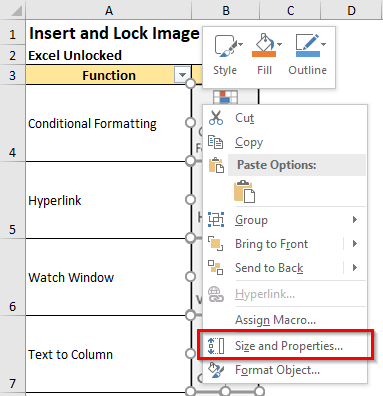
- Right-click on the picture and select Format Picture.

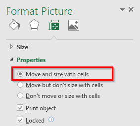
- In the Format Picture pane, select Size & Properties and with the options in Properties, select ‘Move and size with cells’.


That’s It!
Now you can move cells, filter it, or hide it, and the picture will also move/filter/hide.
Try it yourself.. Download the Example File

This could be a useful trick when you have a list of products with their images, and you want to filter certain categories of products along with their images.
You can also use this trick while creating Excel Dashboards.
You May Also Like the Following Excel Tutorials:
- Insert a Picture in a Comment in Excel.
- Insert Line Break in Excel Formula result.
- Picture Lookup Technique using Named Ranges.
- How to Insert Watermark in Excel Worksheets.
- How to Lock Cells in Excel.
While my recommendation is to take advantage of the automation available from Doality.com specifically Picture Manager for Excel
The following vba code should meet your criteria. Good Luck!
This code will insert the image into the chosen cell and will scale it to fit the exact width and height of the cell. For example:
Instructions:
Add a Button Control to your Excel Workbook (click Developer tab, Insert, Active X, Command Button) and then double click on the button in order to get to the VBA Code —>
Sub Button1_Click()
    Dim filePathCell As Range
    Dim imageLocationCell As Range
    Dim filePath As String

    Set filePathCell = Application.InputBox(Prompt:= _
        "Please select the cell that contains the reference path to your image file", _
            Title:="Specify File Path", Type:=8)

     Set imageLocationCell = Application.InputBox(Prompt:= _
        "Please select the cell where you would like your image to be inserted.", _
            Title:="Image Cell", Type:=8)

    If filePathCell Is Nothing Then
       MsgBox ("Please make a selection for file path")
       Exit Sub
    Else
      If filePathCell.Cells.Count > 1 Then
        MsgBox ("Please select only a single cell that contains the file location")
        Exit Sub
      Else
        filePath = Cells(filePathCell.Row, filePathCell.Column).Value
      End If
    End If

    If imageLocationCell Is Nothing Then
       MsgBox ("Please make a selection for image location")
       Exit Sub
    Else
      If imageLocationCell.Cells.Count > 1 Then
        MsgBox ("Please select only a single cell where you want the image to be populated")
        Exit Sub
      Else
        InsertPic filePath, imageLocationCell
        Exit Sub
      End If
    End If
End Sub
Then create your Insert Method as follows (this can follow the button’s code from above):
Private Sub InsertPic(filePath As String, ByVal insertCell As Range)
    Dim xlShapes As Shapes
    Dim xlPic As Shape
    Dim xlWorksheet As Worksheet

    If IsEmpty(filePath) Or Len(Dir(filePath)) = 0 Then
        MsgBox ("File Path invalid")
        Exit Sub
    End If

    Set xlWorksheet = ActiveSheet

    Set xlPic = xlWorksheet.Shapes.AddPicture(filePath, msoFalse, msoCTrue, insertCell.Left, insertCell.Top, insertCell.Width, insertCell.Height)
    xlPic.LockAspectRatio = msoCTrue
End Sub
Do you want to insert an image into a cell? This post is going to show you exactly how to put a picture in a cell in Microsoft Excel!
An Excel cell can contain many different data types such as text, numbers, dates, Booleans, and error values. Until recently, images have not been a data type that you could insert into a cell.
Previously, you could only place the image above the cell and then change the image properties so it moves and resizes with the cells.
There are new features available in Excel that allow you to add images directly inside a cell. This means images are a proper data type and can be used in similar ways to other data such as text or numbers.

Get your copy of the example workbook used in this post and follow along!
Insert an Image in a Cell with Data Types
This first method won’t allow you to get any image embedded in your cell but is a quick and easy way to see images in action using Data Types.
Data types have been available for a while and allow you to pull certain geographical or financial data from the web.
These data types contain many pieces of data inside a single cell. A country data type might contain information about the population, capital, current president, or current prime minister.
The Geography data type in particular also includes a related image. A country, state, or province data type might have the associated flag image included in the data type.
This image can be extracted from the data type into a cell.
This example shows a small list of country names in Excel. These are plain text, so there is nothing special about them until they are converted into geography data types.
You can follow these steps to create a data type and extract the image into the grid.
- Select your list of cells with plain text geographical names such as country names.
- Go to the Data tab.
- Click on the Geography data type.
This will convert the plain-text country names into country data types. You’ll notice the small map icon to the left of the country name which indicates they are now Geography data types.
When you click on this map icon, it will open a pop-up data card that displays all the information contained in the cell. This can include an image of the flag at the top of the card.
Now you will be able to extract the flag image into a cell.
- Select all the data type cells.
- Click on the Extract button that appears at the top right of the selected cells.
- Choose the Image option from the list.
This will extract the data type image into the adjacent cell. You can see this is really a formula =B2.Image that references the cell with the data type by using a dot notation to extract a piece of data from the data type.
💡 Tip: You can copy and paste as values so the image will then be disconnected from the data type.
Insert an Image in a Cell with Power BI Organization Data Types
The Geography data type is perfect if you want a flag image inside your cell!
But what if you want your own custom images added in a cell?
You can build your own custom Organization data type. These can then be used by anyone inside your organization in any of your spreadsheets.
Organization data types also allow you to specify an image URL which can then be extracted to a cell.
⚠️ Warning: This feature requires a Power BI pro license and a table of data that contains a column of image URLs.
- Open the Power BI desktop app.
- Click on the Import data from Excel or choose the Get Data option in the Home tab if your image dataset is not in Excel.
This will open a file picker menu where you can select the Excel file with your image URLs.
- Select the Excel file with your image URLs.
- Press the Open button.
This will open up the Navigator window.
- Select the table or sheet that contains your image URL data.
- Press the Load button.
- Go to the Model view.
- Select the table you loaded.
- Toggle the Is featured table option to Yes in the Properties window pane.
- Add a Description for the table.
- Select a Row Label column from the data. This will be the text displayed in the cell when you’re using this data type in Excel.
- Select a Key column from the data. This should be a unique identifier from the data.
In this example, the Row Label and Key column are the same since the name is what you want to be displayed in Excel and it also uniquely identifies the product.
Now you’ll need to set the column properties for the column of image URLs.
- Go to the Data view.
- Select the column that contains the image URLs.
- Go to the Column tools tab.
- Select Image URL for the Data category.
Now you need to publish this dataset to the Power BI online service so the Organization data type will show up in Excel.
- Go to the Home tab.
- Click on the Publish button.
- Select any workspace other than My workspace.
- Press the Select button.
📝 Note: My workspace is your own personal workspace in Power BI online. No one else will have access and the Organization data type feature does not work with it.
Now you can open Excel and use the new Organization data type. Just make sure Excel is signed into a Microsoft account on the same Microsoft tenant as the workspace you published in Power BI.
- Select some data from your Row Label column.
- Go to the Data tab in the Excel ribbon.
- Click on the button to expand the Data Type shelf.
- Click on your custom data type found in the From your organization section.
This will convert the items into the data type and you will be able to extract the image the same way as with the Geography data type.
In this example, the formula =B2.Image will extract the picture since Image was the name of the column that was set to an Image URL type.
Insert an Image in a Cell with the IMAGE Function
Creating an organization data type is a long process, especially if you only want to add an image inside a cell.
Thankfully there is a better way to insert an image if you have a public web address for it.
The IMAGE function allows you to insert an image in the cell based on a URL.
IMAGE Function Syntax
= IMAGE ( url, alt_text, sizing, height, width )The IMAGE function has the following required arguments.
urlis the web address of the image you want to display in the cell.
The IMAGE function has the following optional arguments.
alt_textis an input for an alternative text for accessibility.sizingis an option to determine how you want the image to fit into the cell.0will fit the cell and maintain the image aspect ratio.1will fill the cell and ignore the image aspect ratio.2will add the image and maintain its original size.3will allow you to enter a custom height and width size for the image.
heightallows you to set the height of the image.widthallows you to set the width of the image.
📝 Note: The height and width arguments are required when sizing is set to 3.
IMAGE Function Example
= IMAGE ( "https://www.howtoexcel.org/wp-content/uploads/2022/10/Insert-Images-Into-Cells.jpg" )The above formula will insert an image from this website. The url argument can be entered as a text string or you can reference a cell that contains the web address.
💡 Tip: You can use an online drive app such as SharePoint or OneDrive to create a public web address that can be used in the IMAGE function. Set the file access as shared with anyone with the link!
Conclusions
Getting an image inside a cell has long been a sought-after feature in Excel. But until recently, there has only been a poor workaround method available.
Now there are some great options available for images in a cell.
You can use the Geography data type quickly get flag images inside cells, and if you want a custom image you can create Organization data types with Power BI.
Images can also be entered into the cell via the IMAGE function. This is a quick and easy way to get any image with a web address into an Excel cell.
Did you know about these features? What are you going to use them for? Let me know in the comments section below!
About the Author
John is a Microsoft MVP and qualified actuary with over 15 years of experience. He has worked in a variety of industries, including insurance, ad tech, and most recently Power Platform consulting. He is a keen problem solver and has a passion for using technology to make businesses more efficient.
How to Insert Pictures Into Excel Cells – Step-by-step (2023)
I bet you know how to insert pictures but do you know how to insert a picture into a cell in Excel?
It’s a fairly simple, but quite unknown method that ultimately locks the image to a cell.
Let me show you how it’s done, step-by-step💡
If you want to tag along, download my Excel sample file here.
How to insert a picture into a cell in Excel
Unlike with some other platforms, you simply can’t copy and paste a picture into an Excel cell.
But I assure you that the process to insert images isn’t difficult.
In fact, the image shown below took only 30 seconds to do.

1. Go to the Insert tab.
2. Click the Illustrations button.
3. Select Picture and choose where the image should come from.
Typically, the image is located on your computer. If that’s the case, select ‘From this device’.

4. Select the images you want to insert.
Tip: You can insert multiple images at the same time.
5. Resize the image to fit the cell and make sure to move the picture into a cell.
Pretty easy, huh?
PRO TIP: KEEP ASPECT RATIO OF IMAGE
When you resize an image in Excel the aspect ratio can get out of hand really quickly, making it look ridiculous.
To keep the aspect ratio intact, make sure to resize it by dragging the handles at the corners of the image.
Don’t drag the handles to the top, bottom, left, or right.

After resizing the images to fit the cells, there’s one problem left:
Resizing the columns or rows where the images reside does not affect the images.
Here’s what I mean:

To solve that, you have to lock the picture into a cell.
How to lock an image to a cell
For the image to resize when you resize the columns or rows, you will have to change its properties.
1. Right-click on the image and select ‘Format Picture’.

This will open the format picture pane where you can change the picture settings.
2. Click on the ‘Size and properties’ button.
3. Expand the ‘Properties’ tab and click ‘Move and size with cells’.

And that’s how you lock a picture into a cell in Excel.
Now, when you resize the cell the image is automatically resized with the cell.
If you insert multiple images, you can select them all by holding down the Shift key while left-clicking each one.
Do this before enabling ‘Move and size with cells’ from the Properties tab in the ‘Format picture pane’ and it’ll be done to all the images at once.
That’s it – What’s next?
As you can see, it’s pretty quick and easy to insert a picture into Excel cells.
The real challenge is making sure that the photo moves and resizes with the cell. Luckily, you can lock the picture into a cell to make that happen.
But to insert an image is only a small part of Microsoft Excel.
Excel can automate calculations, make decisions for you, speed up your daily work, and join data from multiple files in a few seconds.
If you want to get started with all that, you should enroll in my 30-minute free Excel training program that adapts to your Excel skill level.
Click here and sign up with your email address to get instant access to the course.
Other resources
Now that you’re inserting pictures into Excel cells, I got some other relevant resources for you.
Another way of displaying images in your Excel file is by showing them as watermarks. Read all about that here.
Also, if you care about the general look and feel of your spreadsheet, you need to know a few tricks like adding headers and footers, the format painter, and number formats.
Kasper Langmann2023-01-19T12:29:25+00:00
Page load link
Follow this quick guide to insert images in Excel
by Henderson Jayden Harper
Passionate about technology, Crypto, software, Windows, and everything computer-related, he spends most of his time developing new skills and learning more about the tech world. He also enjoys… read more
Updated on December 18, 2022
Reviewed by
Alex Serban

After moving away from the corporate work-style, Alex has found rewards in a lifestyle of constant analysis, team coordination and pestering his colleagues. Holding an MCSA Windows Server… read more
- Before inserting an image in a Microsoft Excel cell, you need to allow the Insert Options to access pictures, charts, etc.
- You can drag and drop images into the Excel cell, but it doesn’t support Windows Explorer.
- Dragging and dropping images into the cell from Microsoft Word is an alternative, so refer to our below procedure.
XINSTALL BY CLICKING THE DOWNLOAD FILE
This software will repair common computer errors, protect you from file loss, malware, hardware failure and optimize your PC for maximum performance. Fix PC issues and remove viruses now in 3 easy steps:
- Download Restoro PC Repair Tool that comes with Patented Technologies (patent available here).
- Click Start Scan to find Windows issues that could be causing PC problems.
- Click Repair All to fix issues affecting your computer’s security and performance
- Restoro has been downloaded by 0 readers this month.
Microsoft Excel is an excellent tool for storing and calculating data. It allows you to insert text, numbers, dates, and error values into the cells. However, a recently added feature now lets you insert images into cells in Excel.
Nonetheless, users report that they can’t insert new cells in Excel when working on the program.
Can I drag and drop images into an Excel cell?
The straightforward answer is Yes. You can drag and drop images into an Excel cell. It allows you to select images directly from a file, and drag and drop it into the desired cell.
However, Microsoft Excel doesn’t support using the drag-and-drop option to copy items from Windows Explorer and insert them in the cells. There’s no definite reason for the restriction, but there is a way around it.
Furthermore, the drag-and-drop option is not a registered feature in Microsoft Excel, so it doesn’t support inserting images directly from open files. Hence, the image must be embedded in a file to be viewed in Excel.
How do I insert a picture into a selection cell?
Go through the following before proceeding with the guide below:
- Move the necessary images to an identifiable file.
- Ensure Word is running on your PC.
- Back up your current work on Excel before trying to insert any image.
The above checks will help prepare the necessary items to insert images in the Excel cell. Follow the steps below to start inserting.
1. Via the Insert tab
1.1 Allow the Insert options in Excel
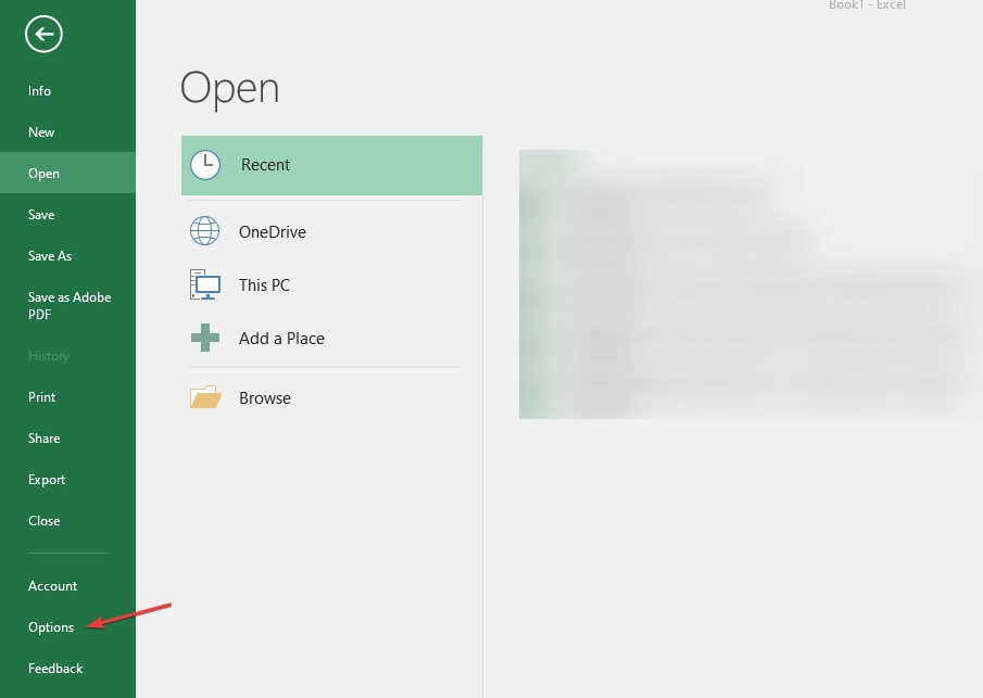
- Launch Microsoft Excel and click on Files in the top-right corner.
- Click on Options.

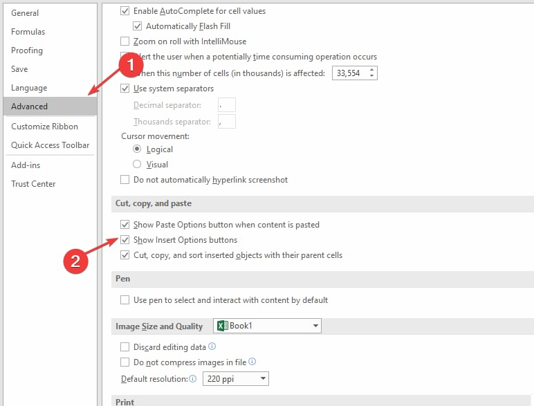
- Then select the Advanced tab on the left pane. Go to the Cut, Copy and Paste tab, then check the box for the Show Insert Options button.

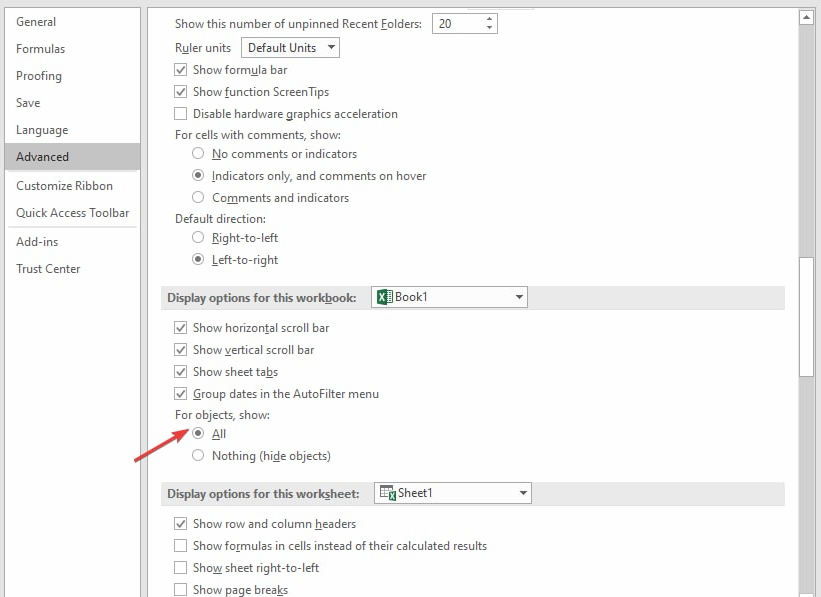
- Scroll down to the Display options for this workbook tab, check the box for All, then click the OK button.

The steps above allow you to access and use the Insert Options to cut, copy, and paste images, charts, etc., into the Excel cells.
1.2 Use the Insert feature to add an Image into a cell in Excel
- Go to the cell where you want to insert the image, click the Insert tab on the toolbar, tap the Illustration button, and select Picture.

- Select an option from the Insert Picture From section, choose the image you want, then click the Insert button.
- The picture will appear on the spreadsheet. Drag the small circles at the edges to modify the picture size until it is small enough to fit into the cell.

- Save your Excel file and continue your work.
The Insert Option allows you to access pictures and other items to add to the Excel cells you’re currently working on. Check our article on what to do if the toolbar is missing in Microsoft Excel.
- Excel Running Slow? 4 Quick Ways to Make It Faster
- Fix: Excel Stock Data Type Not Showing
2. Insert an image into an Excel cell by dragging and dropping
- Launch Microsoft Word, and create a new document.
- Navigate to the directory of the image, and copy and paste it into the Word document.

- Launch Microsoft Excel and enter the cell you want to insert the image.
- Go to Word, click and hold on to the image, drag it across to the Excel spreadsheet, then drop it into the cell.
- If needed, drag the small circles at the edges to modify the picture size until it is small enough to fit into the cell.


Since Microsoft Excel doesn’t support dragging and dropping from Windows Explorer, using Microsoft Word is the best alternative. It allows you to drag images and drop them into your desired cells easily.
Read how to fix Microsoft Word not working on Windows 11.
Our readers can also check our guide on fixing corrupt Excel cells that may cause problems with their activities on Excel. Even more, you can read about what to do if you run into too many different cell formats error in Excel.
If you have further questions or suggestions on this guide, kindly drop them in the comments section.
Still having issues? Fix them with this tool:
SPONSORED
If the advices above haven’t solved your issue, your PC may experience deeper Windows problems. We recommend downloading this PC Repair tool (rated Great on TrustPilot.com) to easily address them. After installation, simply click the Start Scan button and then press on Repair All.
![]()
Newsletter
Excel is generally said to be used for making complex calculations with formula and other functions. However, many times you may need to insert an image and picture in excel worksheet to give a visual representation of what is written in the excel. In this blog, we would learn how to insert an image or picture in an Excel cell. We would also unlock the technique to lock an image or picture into an excel cell such that when we resize or filter the cells containing the image, the picture automatically gets resized or filtered along with that cell.
This technique is very useful for creating a business product catalog with the product name in a cell and its image in the adjacent cell.
The below demonstration is the glimpse of what we are going to achieve in this blog.
Please download the practice file using ‘Download’ button below.
Let us now first unlock the technique to insert and resize the image in a cell in Excel.
Follow the below steps to add an image in excel:
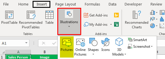
Under the excel ribbon options, click on the ‘Insert‘ tab and under the ‘Illustration‘ group, click on the ‘Pictures‘ button.
As a result, the ‘Insert Picture‘ dialog box would appear on your screen. Navigate to the path which contains the pictures, select all of them, and then click on the ‘Insert’ button. Refer to the image below:
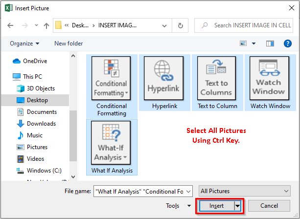
You would notice that the selected pictures gets inserted in to the excel worksheet.
The next step now is to place the pictures in the relevant cells in Excel. To do this, left-click on the picture and drag it to the relevant cell and finally release the mouse cursor. Refer to the below demonstration.
Once the pictures are put in relevant cells, the next step is to resize it to fit the image or picture in the cell. The two most common ways that almost everybody is aware of are-
- By adjusting the picture borders by using the circles on the edges and borders of the image.
- By manually entering the height and width of the picture under the ‘Format’ tab.
Interesting Way to Exactly Fit Image or Picture to Cell Borders
The third and the interesting way to exactly fit the image or picture to excel cell walls is this one –
- Click on the image, and press and hold the ALT key on your keyboard.
- Do not release the ALT press, and simply drag the image toward the top-left corner of the cell. As you come closure to the cell corner, the image would automatically stick exactly to the cell’s top-left corner.
- Again, do not release the ALT press, and drag the bottom-right corner of the image toward the bottom-right corner of cell. See the demonstration below.
With this, we have completed the technique of inserting an image into the cell in Excel.
Now, let us perform one small activity, to understand something interesting.
Simply, try to resize the column with contains the images (column B). You would notice that the image would not automatically resize along with the cell. It remains intact at the same position. Similarly, if you filter column A, the images in column B would not accordingly filter, as demonstrated below:
Reason – At this point in time, the picture is not a part of the cell, but it is placed above the cell in the worksheet.
To lock the picture into the cell in Excel, so that it can be resized and filtered along with the cell, follow the below section of the blog.
Related Post : How to Lookup on Picture in Excel
How to Lock Picture or Image Into Excel Cell
To lock the image or picture in excel cell, we need to change the properties of the image. Below steps would help you in this:
Lock Picture / Image Into Excel Cell
- Select All Images
Select any picture and press Ctrl + A to select all the images in the worksheet.
- Size and Properties
Right click on any of the image and click on the option – ‘Size and Properties’.

- Format Picture > Move and Size with Cell Option
A ‘Format Picture’ pane would appear on the right of the worksheet. Expand the ‘Properties’ section, and select the radio button ‘Move and Size with Cells‘ and that’s it, the image is now the part of the cell.

This means, if you now resize the cell, the image would also get resized accordingly. Similarly, the images in the filtered cell would also hide along with the cell.
With this, we have reached the end of this blog. Now, make your own business catalog with the images as a part of your cell. Share your views and comments in the comment section.
RELATED POSTS
-
AutoFit Column Width and Row Height in Excel
-
How to Insert Picture or Image in Excel Comment
-
How to Wrap Text in Excel Cell
-
Assign Macro to Image and CheckBox
-
Change Row Height, Column Width VBA (Autofit)
-
Apply Border to Cells using VBA in Excel
Содержание
- Insert a Picture/Image in Excel Cell
- How to Insert a Picture/Image in Excel Cell?
- Change Image Size According to Cell Size in Excel
- How to Create an Excel Dashboard with Images?
- Things to Remember
- Recommended Articles
- Excel IMAGE function — quick way to insert picture in cell with formula
- Excel IMAGE function
- IMAGE function availability
- Basic IMAGE formula in Excel
- How to insert pictures in Excel cells — formula examples
- How to make a product list with pictures in Excel
- How to return an image based on another cell value
- How to make a dropdown with pictures in Excel
- Excel IMAGE function known issues and limitations
Insert a Picture/Image in Excel Cell


How to Insert a Picture/Image in Excel Cell?
Table of contents
Inserting a picture or an image into an Excel cell is easy.
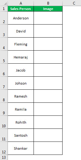
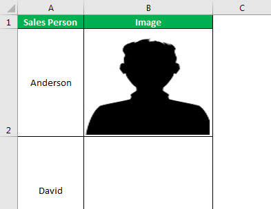
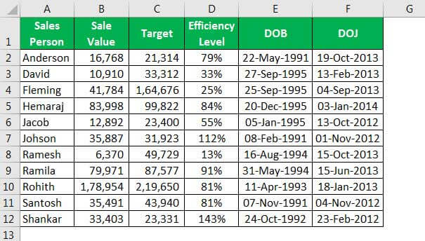
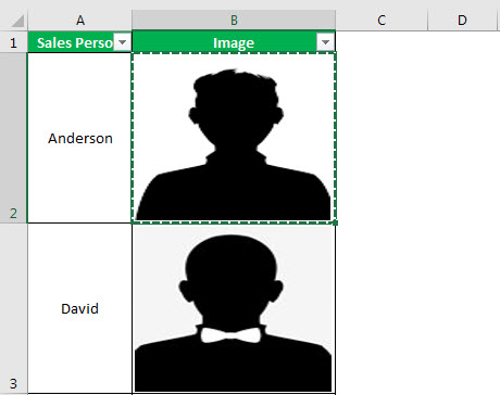
- For example, we have sales employees’ names in the Excel file. Below is the list.

We have their images on the computer hard disk.
We want to bring the image against each person’s name, respectively.
Note: All the images are dummy. We can download them from Google directly.
We must copy the above list of names and paste it into Excel. Make the row height as 36 and column width in Excel 14.3.
Go to the Insert tab and click on Pictures.
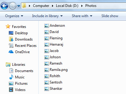
Once we click on Pictures, it asks us to choose the picture folder location from the computer. So, we must select the location and the pictures we want to insert.
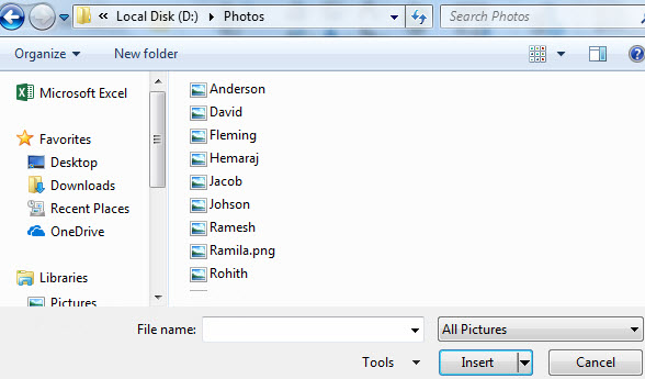
We can insert a picture one by one in an Excel cell, or we can insert it in one shot. To insert at one go, we need to be sure which represents who. So, we are going to insert them one by one. Select the image we want to insert and click on Insert.

Now, we can see the image in our Excel file.
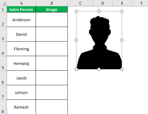
This picture is not yet ready to use. We need to resize this. We must select the picture and resize it using the drag and drop option in Excel from the corner edges of the image, or we can resize the height and width under the Format tab.
Note: Modify the row height as 118 and column width as 26.

To fit the picture to the cell size, we must hold the ALT key and drag the picture corners. After that, it will automatically fit the cell size.
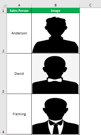
Like this, we must repeat this task for all the employees.
Change Image Size According to Cell Size in Excel
Now, we need to fit these images to the cell size. Whenever the cell width or height changes, the picture also should change accordingly.
- Step 1: First, we must select one image and press “Ctrl + A.” It will choose all the images in the active worksheet. (Make sure all the images are selected).
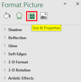
- Step 2:Now, press “Ctrl + 1.” It will open up the “Format” option on the right-hand side of the screen. Note: We are using Excel 2016 version.

- Step 3: Under “Format Picture,” select “Size & Properties.”
- Step 4: Click on “Properties” and select the option “Move and size with cells.”
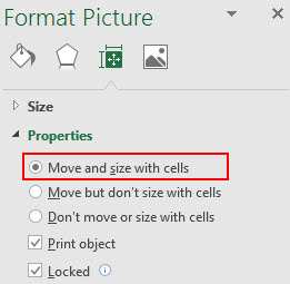
- Step 5: We have locked the images to their respective cell sizes. It is dynamic now. As the cell changes, images are also kept changing.
How to Create an Excel Dashboard with Images?
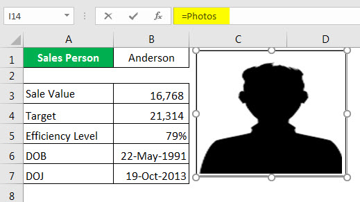
We have created a master sheet that contains all the details of the employees.
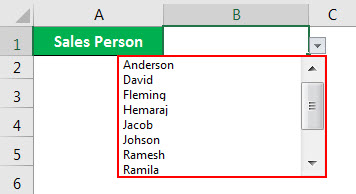
- Step 1: The sheet creates a dropdown list of employee lists in the dashboard.
- Step 2: We must Apply VLOOKUPApply VLOOKUPThe VLOOKUP excel function searches for a particular value and returns a corresponding match based on a unique identifier. A unique identifier is uniquely associated with all the records of the database. For instance, employee ID, student roll number, customer contact number, seller email address, etc., are unique identifiers.read more to get the “Sales Value,” “Target,” “Efficiency Level,” “DOB,” and “DOJ” from the “Employee Details” sheet.
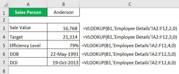
The values will be automatically updated as you change the name from the drop-down.
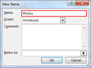
- Step 3: The big part is getting the employee’s photo selected from the drop-down. For this, we need to create a “Name Manager.”
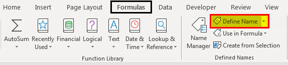
Go to “FORMULAS” > “Define Name” in Excel.
Things to Remember
- We must make the image adjustment that fits or changes the cell movement.
- Create a master sheet containing all the consolidated data to create a dashboard.
- We must use the “ALT” key to adjust the image to the extreme corners of the cell.
Recommended Articles
This article is a guide to Insert a Picture/Image in Excel Cell. We discussed inserting a picture or an image into a cell in Excel and creating a dashboard with images in Excel, an example, and a downloadable Excel sheet. You can learn more about Excel from the following articles: –
Источник
Excel IMAGE function — quick way to insert picture in cell with formula
 by Alexander Frolov, updated on March 1, 2023
Learn a new amazingly simple way to insert a picture into a cell by using the IMAGE function.
Microsoft Excel users have inserted pictures into worksheets for years, but that required quite a lot of effort and patience. Now, that’s finally over with. With the newly introduced IMAGE function, you can insert a picture in a cell with a simple formula, place images within Excel tables, move, copy, resize, sort and filter cells with pictures just like normal cells. Instead of floating on top of a spreadsheet, your images are now its integral part.
Excel IMAGE function
The IMAGE function in Excel is designed to insert pictures into cells from a URL. The following file formats are supported: BMP, JPG/JPEG, GIF, TIFF, PNG, ICO, and WEBP.
The function takes a total of 5 arguments, of which only the first one is required.
Source (required) — the URL path to the image file that uses the «https» protocol. Can be supplied in the form of a text string enclosed in double quotes or as a reference to the cell containing the URL.
Alt_text (optional) — the alternative text describing the picture.
Sizing (optional) — defines the image dimensions. Can be one of these values:
- 0 (default) — fit the picture in the cell maintaining its aspect ratio.
- 1 — fill the cell with the image ignoring its aspect ratio.
- 2 — keep the original image size, even if it goes beyond the cell boundary.
- 3 — set the image’s height and width.
Height (optional) — the image height in pixels.
Width (optional) — the image width in pixels.
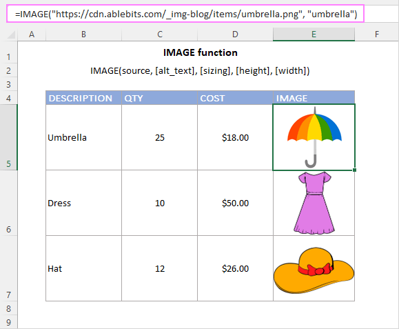
IMAGE function availability
IMAGE is a new function, which is currently available only to Microsoft 365 users for Windows, Mac and Android as well as in Excel for the web.
Basic IMAGE formula in Excel
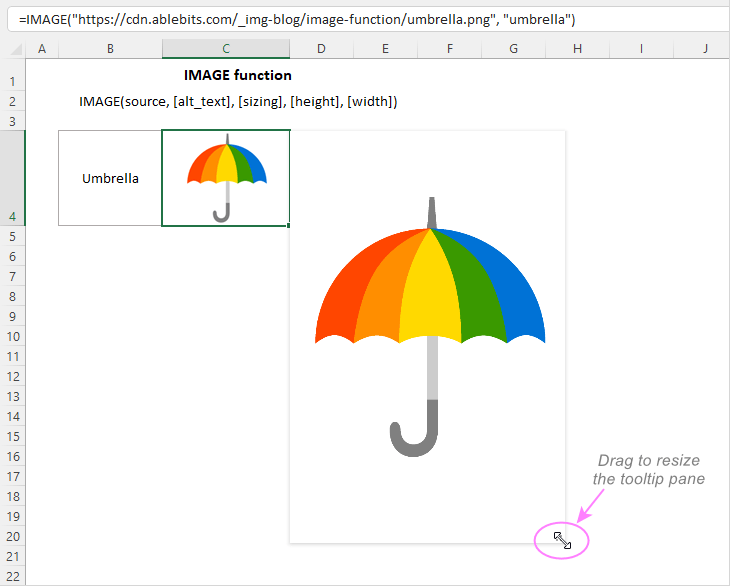
To create an IMAGE formula in its simplest form, it is sufficient to supply only the 1 st argument that specifies the URL to the image file. Please remember that only HTTPS addresses are allowed and not HTTP. A supplied URL should be enclosed in double quotes just like a regular text string. Optionally, in the 2 nd argument, you can define an alternative text describing the image.
Omitting or setting the 3rd argument to 0 forces the image to fit into the cell, maintaining the width to height ratio. The image will adjust automatically when the cell is resized:
When you hover over the cell with an IMAGE formula, the tooltip pops out. The minimum size of the tooltip pane is preset. To make it bigger, drag the lower-right corner of the pane like shown below.
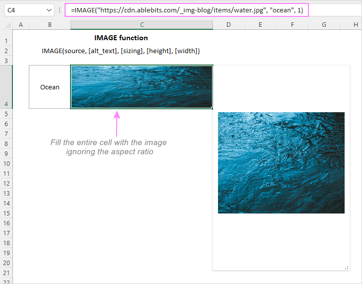
To fill the whole cell with an image, set the 3 rd argument to 1. For example:
=IMAGE(«https://cdn.ablebits.com/_img-blog/image-function/items/water.jpg», «ocean», 1)
Normally, this works nicely for abstract arts images that look well with almost any width-to-height ratio.
If you decide to set the image’s height and width (4 th and 5 th argument, respectively), make sure your cell is big enough to accommodate the original size picture. If not, only part of the image will be visible.
Once the picture is inserted, you can get it copied to another cell by simply copying the formula. Or you can reference a cell with an IMAGE formula just like any other cell in your worksheet. For example, to copy a picture from C4 to D4, enter the formula =C4 in D4.
How to insert pictures in Excel cells — formula examples
Introducing the IMAGE function in Excel has «unlocked» many new scenarios that were previously impossible or highly complicated. Below you will find a couple of such examples.
How to make a product list with pictures in Excel
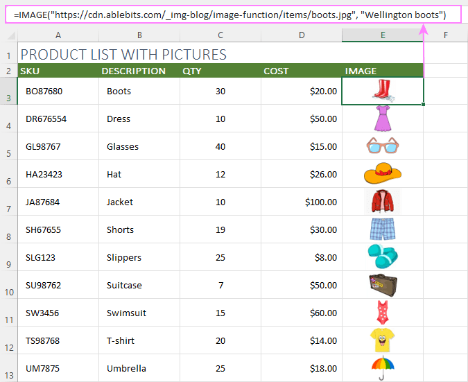
With the IMAGE function, creating a product list with pictures in Excel becomes incredibly easy. The steps are:
- Make a new product list in your worksheet. Or import an existing one from an external database as a csv file. Or use a product inventory template available in Excel.
- Upload the product images to some folder on your website.
- Construct the IMAGE formula for the first item and enter it in the topmost cell. In the formula, only the first argument (source) needs to be defined. The second argument (alt_text) is optional.
- Copy the formula across the below cells in the Image column.
- In each IMAGE formula, change the file name and the alternative text if you’ve supplied it. As all the pictures were uploaded to the same folder, this is the only change that needs to be made.
In this example, the below formula goes to E3:
=IMAGE(«https://cdn.ablebits.com/_img-blog/image-function/items/boots.jpg», «Wellington boots»)
As a result, we’ve got the following product list with pictures in Excel:
How to return an image based on another cell value
For this example, we are going to create a drop-down list of items and extract a related image into a neighboring cell. When a new item is selected from the dropdown, the corresponding picture will appear next to it.
- As we aim at a dynamic dropdown that expands automatically when new items are added, our first step is to convert the dataset to an Excel table. The fastest way is by using the Ctrl + T shortcut. Once the table is created, you can give any name you want to it. Ours is named Product_list.
- Create two named ranges for the Item and Image columns, not including the column headers:
- Items referring to =Product_list[ITEM]
- Images referring to =Product_list[IMAGE]

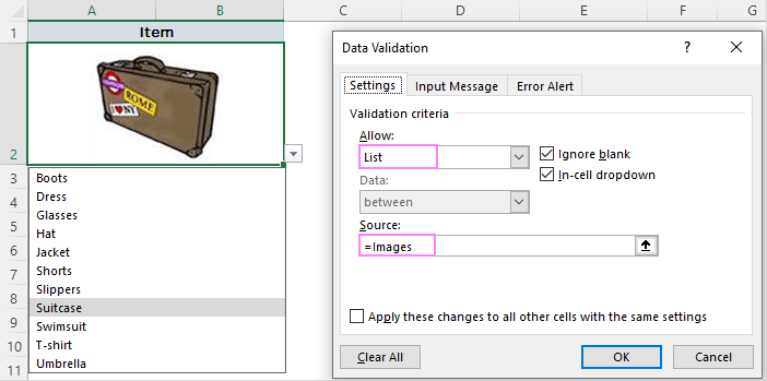
With the cell for the dropdown selected, navigate to the Data tab >Date Tools group, click Data Validation, and configure the dropdown list based on an Excel name. In our case, =Items is used for Source.

In the cell designated for an image, enter the following XLOOKUP formula:
=XLOOKUP(A2, Product_list[ITEM], Product_list[IMAGE])
Where A2 (lookup_value) is the dropdown cell.
As we look up in a table, the formula uses structured references such as:
- Lookup_array — Product_list[ITEM] which says to search for the lookup value in the column named ITEM.
- Return_array — Product_list[IMAGE]) which says to return a match from the column named IMAGE.
The result will look something like this:

And here’s our dropdown list with related pictures in action — as soon as an item is selected in A2, its image is immediately displayed in B2: 
How to make a dropdown with pictures in Excel
In earlier Excel versions, there was no way to add pictures to a drop down list. The IMAGE function has changed this. Now, you can make a dropdown of pictures in 4 quick steps:
- Start with defining the two names for your dataset. In our case, the names are:
- Product_list — the source table (A10:E20 in the screenshot below).
- Images — refers to the IMAGE column in the table, not including the header.
For detailed instructions, please see How to define a name in Excel.
Additionally, you can retrieve more information about the selected item with the help of these formulas:
Get the item name:
=XLOOKUP($A$2, Product_list[IMAGE], Product_list[ITEM])
Pull the quantity:
=XLOOKUP($A$2, Product_list[IMAGE], Product_list[QTY])
Extract the cost:
=XLOOKUP($A$2, Product_list[IMAGE], Product_list[COST])
As the source data is in a table, the references use a combination of the table and column names. Learn more about table references.
The resulting drop down with images is shown in the screenshot:

Excel IMAGE function known issues and limitations
Currently, the IMAGE function is in the beta testing stage, so having a few issues is normal and expected 🙂
- Only images saved on external «https» websites can be used.
- Pictures saved on OneDrive, SharePoint and local networks are not supported.
- If the website where the image file is stored requires authentication, the image will not render.
- Switching between Windows and Mac platforms may cause issues with image rendering.
- While the GIF file format is supported, it is displayed in a cell as a static image.
That’s how you can insert a picture in a cell using the IMAGE function. I thank you for reading and hope to see you on our blog next week!
Источник
You can download this Insert Image Excel Cell Template here – Insert Image Excel Cell Template
Table of contents
- How to Insert a Picture/Image in Excel Cell?
- Change Image Size According to Cell Size in Excel
- How to Create an Excel Dashboard with Images?
- Things to Remember
- Recommended Articles
Inserting a picture or an image into an Excel cell is easy.
- For example, we have sales employees’ names in the Excel file. Below is the list.

- We have their images on the computer hard disk.

We want to bring the image against each person’s name, respectively.Note: All the images are dummy. We can download them from Google directly.
- We must copy the above list of names and paste it into Excel. Make the row height as 36 and column width in Excel 14.3.

- Go to the Insert tab and click on Pictures.

- Once we click on Pictures, it asks us to choose the picture folder location from the computer. So, we must select the location and the pictures we want to insert.

- We can insert a picture one by one in an Excel cell, or we can insert it in one shot. To insert at one go, we need to be sure which represents who. So, we are going to insert them one by one. Select the image we want to insert and click on Insert.

- Now, we can see the image in our Excel file.

- This picture is not yet ready to use. We need to resize this. We must select the picture and resize it using the drag and drop option in Excel from the corner edges of the image, or we can resize the height and width under the Format tab.
Note: Modify the row height as 118 and column width as 26.

- To fit the picture to the cell size, we must hold the ALT key and drag the picture corners. After that, it will automatically fit the cell size.

- Like this, we must repeat this task for all the employees.

Change Image Size According to Cell Size in Excel
Now, we need to fit these images to the cell size. Whenever the cell width or height changes, the picture also should change accordingly.
- Step 1: First, we must select one image and press “Ctrl + A.” It will choose all the images in the active worksheet. (Make sure all the images are selected).
- Step 2: Now, press “Ctrl + 1.” It will open up the “Format” option on the right-hand side of the screen. Note: We are using Excel 2016 version.
- Step 3: Under “Format Picture,” select “Size & Properties.”
- Step 4: Click on “Properties” and select the option “Move and size with cells.”
- Step 5: We have locked the images to their respective cell sizes. It is dynamic now. As the cell changes, images are also kept changing.
How to Create an Excel Dashboard with Images?
We can create a dashboard using these pictures. Follow the below steps to create an excel dashboardThe dashboard in excel is an enhanced visualization tool that provides an overview of the crucial metrics and data points of a business. By converting raw data into meaningful information, a dashboard eases the process of decision-making and data analysis.read more.
We have created a master sheet that contains all the details of the employees.
- Step 1: The sheet creates a dropdown list of employee lists in the dashboard.
- Step 2: We must Apply VLOOKUPThe VLOOKUP excel function searches for a particular value and returns a corresponding match based on a unique identifier. A unique identifier is uniquely associated with all the records of the database. For instance, employee ID, student roll number, customer contact number, seller email address, etc., are unique identifiers.
read more to get the “Sales Value,” “Target,” “Efficiency Level,” “DOB,” and “DOJ” from the “Employee Details” sheet.
The values will be automatically updated as you change the name from the drop-down.
- Step 3: The big part is getting the employee’s photo selected from the drop-down. For this, we need to create a “Name Manager.”
Go to “FORMULAS” > “Define Name” in Excel.
- Step 4: Give a name to the “Name Manager.”
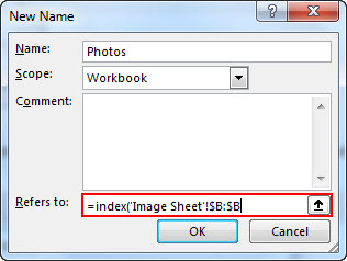
- Step 5: In “Refers to” type “equal (=) sign” and enter the INDEX formulaThe INDEX function in Excel helps extract the value of a cell, which is within a specified array (range) and, at the intersection of the stated row and column numbers.read more.
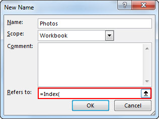
- Step 6: The first argument of the INDEX functionThe INDEX function in Excel helps extract the value of a cell, which is within a specified array (range) and, at the intersection of the stated row and column numbers.read more is to select the whole B column in the “Image Sheet.”
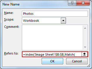
- Step 7: Now, enter comma (,) and open one more function MATCHThe MATCH function looks for a specific value and returns its relative position in a given range of cells. The output is the first position found for the given value. Being a lookup and reference function, it works for both an exact and approximate match. For example, if the range A11:A15 consists of the numbers 2, 9, 8, 14, 32, the formula “MATCH(8,A11:A15,0)” returns 3. This is because the number 8 is at the third position.
read more.
- Step 8: We must select the first argument as “Employee Name” in the “Dashboard” Sheet. (dropdown cell).

- Step 9: Next argument, select the entire first column in “Image Sheet,” enter “zero” as the next argument, and close two brackets.
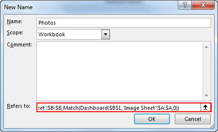
- Step 10: Click on “OK.” Now, we have created a name manager for our photos.
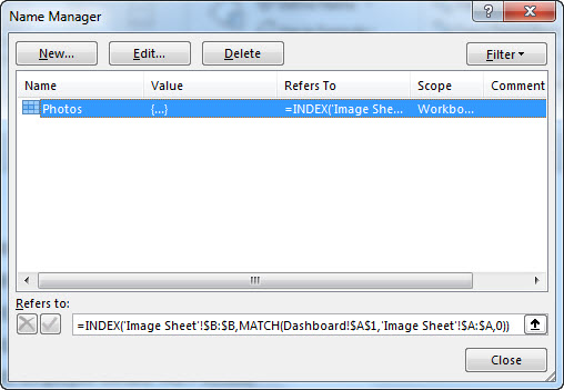
- Step 11: Now go to the “Image” sheet and copy cell B2.
- Step 12: Now go to the “Dashboard” Sheet and paste it as “Linked Picture.”
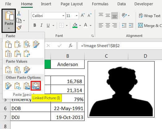
- Step 13: Now, we have an image. We must select the image in the formula and change the link to our Name ManagerThe name manager in Excel is used to create, edit, and delete named ranges. For example, we sometimes use names instead of giving cell references. By using the name manager, we can create a new reference, edit it, or delete it.read more name, Photos.
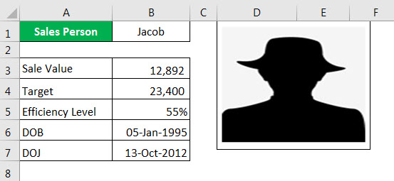
- Step 14: Press the “Enter” key to complete the process. We can change the image. It may vary according to the name we have selected.
Things to Remember
- We must make the image adjustment that fits or changes the cell movement.
- Create a master sheet containing all the consolidated data to create a dashboard.
- We must use the “ALT” key to adjust the image to the extreme corners of the cell.
Recommended Articles
This article is a guide to Insert a Picture/Image in Excel Cell. We discussed inserting a picture or an image into a cell in Excel and creating a dashboard with images in Excel, an example, and a downloadable Excel sheet. You can learn more about Excel from the following articles: –
- Excel KPI Dashboard
- VLookup with Match Formula
- Proper Formula Excel
- Examples of Flowchart in Excel