
Excel for Microsoft 365 Excel 2021 Excel 2019 Excel 2016 Excel 2013 Excel 2010 Excel 2007 More…Less
Let’s say you want to ensure that a column contains text, not numbers. Or, perhapsyou want to find all orders that correspond to a specific salesperson. If you have no concern for upper- or lowercase text, there are several ways to check if a cell contains text.
You can also use a filter to find text. For more information, see Filter data.
Find cells that contain text
Follow these steps to locate cells containing specific text:
-
Select the range of cells that you want to search.
To search the entire worksheet, click any cell.
-
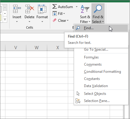
On the Home tab, in the Editing group, click Find & Select, and then click Find.

-
In the Find what box, enter the text—or numbers—that you need to find. Or, choose a recent search from the Find what drop-down box.
Note: You can use wildcard characters in your search criteria.
-
To specify a format for your search, click Format and make your selections in the Find Format popup window.
-
Click Options to further define your search. For example, you can search for all of the cells that contain the same kind of data, such as formulas.
In the Within box, you can select Sheet or Workbook to search a worksheet or an entire workbook.
-
Click Find All or Find Next.
Find All lists every occurrence of the item that you need to find, and allows you to make a cell active by selecting a specific occurrence. You can sort the results of a Find All search by clicking a header.
Note: To cancel a search in progress, press ESC.
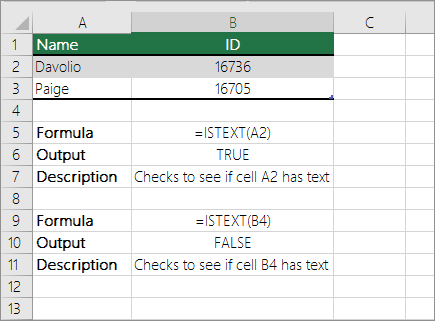
Check if a cell has any text in it
To do this task, use the ISTEXT function.
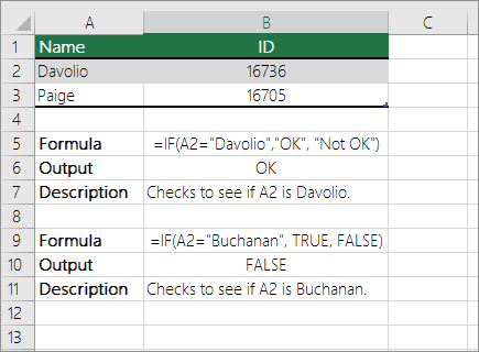
Check if a cell matches specific text
Use the IF function to return results for the condition that you specify.
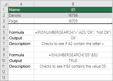
Check if part of a cell matches specific text
To do this task, use the IF, SEARCH, and ISNUMBER functions.
Note: The SEARCH function is case-insensitive.
Need more help?
A while back Vernon asked me how he could search one cell and compare it to a list of words. If any of the words in the list existed then return the matching word.
Ugh, I’ve written that 3 times and I’m not sure it’s any clearer…let’s look at an example.
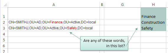
I’ve highlighted the matching words in column A red.
What we want Excel to do is to check the text string in column A to see if any of the words in our list in H1:H3 are present, if they are then return the matching word. Note: I’ve given cells H1:H3 the named range ‘list’.
There are a few ways we can tackle this so let’s take a look at our options.
Warning: this is quite an advanced topic which requires an array formula to solve it.
Update: It’s easier and more robust to use Power Query to search for text strings, including case and non-case sensitive searches.
Non-Case Sensitive Matching
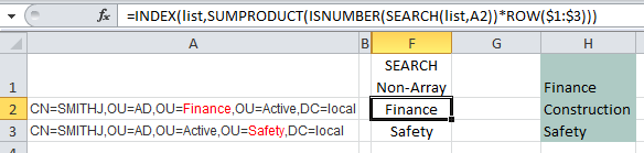
If you aren’t worried about case sensitive matches then you can use the SEARCH function with INDEX, SUMPRODUCT and ISNUMBER like this:
=INDEX(list,SUMPRODUCT(ISNUMBER(SEARCH(list,A2))*ROW($1:$3)))
In English our formula reads:
SEARCH cell A2 to see if it contains any words listed in cells H1:H3 (i.e. the named range ‘list’) and return the number of the character in cell A2 where the word starts. Our formula becomes:
=INDEX(list,SUMPRODUCT(ISNUMBER({20;#VALUE!;#VALUE!})*ROW($1:$3)))
i.e. in cell A2 the ‘F’ in the word ‘Finance’ starts in position 20.
Now using ISNUMBER test to see if the SEARCH formula returns any numbers (if it does it means there is a match). ISNUMBER will return TRUE if there is a number and FALSE if not (this gives us a list of Boolean TRUE or FALSE values). Our formula becomes:
=INDEX(list,SUMPRODUCT({TRUE;FALSE;FALSE}*ROW($1:$3)))
Use the ROW function to return an array of numbers {1;2;3} (see notes below on why I’ve used ROW in this formula). Our formula becomes:
=INDEX(list,SUMPRODUCT({TRUE;FALSE;FALSE}*{1;2;3}))
When you multiply Boolean TRUE/FALSE values they become their numeric equivalents i.e. TRUE = 1 and FALSE = 0. So our formula evaluates this ({TRUE;FALSE;FALSE}*{1;2;3}) like so: {1*1, 0*2, 0*3} and our formula becomes:
=INDEX(list,SUMPRODUCT({1;0;0}))
SUMPRODUCT simply sums the values {1+0+0} which gives us 1. Note: by using SUMPRODUCT we are avoiding the need for an array formula that requires CTRL+SHIFT+ENTER. Our formula becomes:
=INDEX(list,1)
Index can now go ahead and return the 1st value in the range of cells H1:H3 which is ‘Finance’.
Note: the above formula will not work if a match isn’t found. If you want to return an error if a match isn’t found then you can use this variation:
=INDEX(list,IF(SUMPRODUCT(--ISNUMBER(SEARCH(list,A2)))<>0,SUMPRODUCT(ISNUMBER(SEARCH(list,A2))*ROW($1:$3)),NA()))
Not as elegant, is it? In which case you might prefer one of the array formulas below.
Notes about the ROW Function:
The ROW function simply returns the row number of a reference. e.g. ROW(A2) would return 2. When used in an array formula it will return an array of numbers. e.g. ROW(A2:A4) will return {2;3;4}. We can also give just the row reference(s) to the ROW function like so ROW(2:4).
In this formula we have used ROW to simply return an array of values {1;2;3} that represent the items in our ‘list’ i.e. Finance is 1, Construction is 2 and Safety is 3. Alternatively we could have typed {1;2;3} direct in our formula, or even referenced the named range like this ROW(list).
So you see using the ROW function is just a quick and clever way to generate an array of numbers.
What you must bear in mind when using the ROW function for this purpose is that we need a list of numbers from 1 to 3 because there are 3 words in our list and we’re trying to find the position of the matching word.
In this example the formula; ROW(list) will also work because our list happens to start on row 1 but if we were to start ‘list’ on row 2 we would come unstuck because ROW(list) would return {2;3;4} i.e. ‘list’ would actually reference cells H2:H4.
So, don’t get confused into thinking the ROW part of the formula is simply referencing the list or range of cells where the list is, the important point is that the ROW formula returns an array of numbers and we’re using those numbers to represent the number of rows in the ‘list’ which must always start with 1.
Functions Used
INDEX
SEARCH or FIND
ISNUMBER
SUMPRODUCT
ROW — Explained above.
Case Sensitive Matching
[updated Dec 5, 2013]
If your search is case sensitive then you not only need to replace SEARCH with FIND, but you also need to introduce an IF formula like so:
=INDEX(list,IF(SUMPRODUCT(ISNUMBER(FIND(list,A2))*ROW($1:$3))<>0,SUMPRODUCT(ISNUMBER(FIND(list,A2))*ROW($1:$3)),NA()))
Unfortunately it’s not as simple or elegant as the first non-case sensitive search. Instead the array formulas below are nicer
Array Formula Options
Below are some array formula options to achieve the same result. They use LARGE instead of SUMPRODUCT, and as a result you need to enter these by pressing CTRL+SHIFT+ENTER.
Non-case Sensitive:
[updated Dec 5, 2013]
=INDEX(list,LARGE(IF(ISNUMBER(SEARCH(list,A2)),ROW($1:$3)),1)) Press CTRL+SHIFT+ENTER
Case sensitive:
[updated Dec 5, 2013]
=INDEX(list,LARGE(IF(ISNUMBER(FIND(list,A2)),ROW($1:$3)),1)) Press CTRL+SHIFT+ENTER
Download
Enter your email address below to download the sample workbook.
By submitting your email address you agree that we can email you our Excel newsletter.
Thanks
Special thanks to Roberto for suggesting the ‘updated’ formulas above.
Normally, If you want to write an IF formula for text values in combining with the below two logical operators in excel, such as: “equal to” or “not equal to”.
Table of Contents
- Excel IF function check if a cell contains text(case-insensitive)
- Excel IF function check if a cell contains text (case-sensitive)
- Excel IF function check if part of cell matches specific text
- Excel IF function with Wildcards text value
- Related Formulas
- Related Functions
Excel IF function check if a cell contains text(case-insensitive)
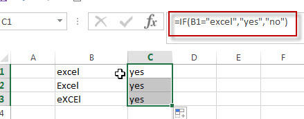
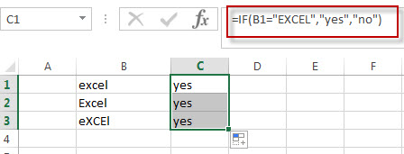
By default, IF function is case-insensitive in excel. It means that the logical text for text values will do not recognize case in the IF formulas. For example, the following two IF formulas will get the same results when checking the text values in cells.
=IF(B1="excel","yes","no")
=IF(B1="EXCEl","yes","no")
The IF formula will check the values of cell B1 if it is equal to “excel” word, If it is TRUE, then return “yes”, otherwise return “no”. And the logical test in the above IF formula will check the text values in the logical_test argument, whatever the logical_test values are “Excel”, “eXcel”, or “EXCEL”, the IF formula don’t care about that if the text values is in lowercase or uppercase, It will get the same results at last.
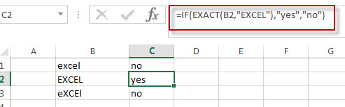
Excel IF function check if a cell contains text (case-sensitive)
If you want to check text values in cells using IF formula in excel (case-sensitive), then you need to create a case-sensitive logical test and then you can use IF function in combination with EXACT function to compare two text values. So if those two text values are exactly the same, then return TRUE. Otherwise return FALSE.
So we can write down the following IF formula combining with EXACT function:
=IF(EXACT(B1,"excel"),"yes","no")
Excel IF function check if part of cell matches specific text
If you want to check if part of text values in cell matches the specific text rather than exact match, to achieve this logic text, you can use IF function in combination with ISNUMBER and SEARCH Function in excel.
Both ISNUMBER and SEARCH functions are case-insensitive in excel.
=IF(ISNUMBER(SEARCH("x",B1)),"good","bad")
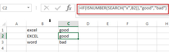
For above the IF formula, it will Check to see if B1 contain the letter x.
Also, we can use FIND function to replace the SEARCH function in the above IF formula. It will return the same results.
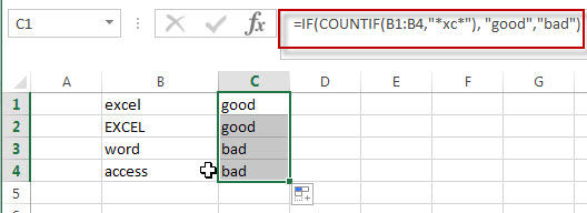
Excel IF function with Wildcards text value
If you wan to use wildcard charcter in an IF formula, for example, if any of the values in column B contains “*xc*”, then return “good”, others return “bad”. You can not directly use the wildcard characters in IF formula, and we can use IF function in combination with COUNTIF function. Let’s see the following IF formula:
=IF(COUNTIF(B1:B4,"*xc*"), "good","bad")
- Excel IF Function With Numbers
If you want to check if a cell values is between two values or checking for the range of numbers or multiple values in cells, at this time, we need to use AND or OR logical function in combination with the logical operator and IF function…
- Excel EXACT function
The Excel SEARCH function returns the number of the starting location of a substring in a text string.The syntax of the EXACT function is as below:= EXACT (text1,text2)… - Excel COUNTIF function
The Excel COUNTIF function will count the number of cells in a range that meet a given criteria.= COUNTIF (range, criteria) … - Excel ISNUMBER function
The Excel ISNUMBER function returns TRUE if the value in a cell is a numeric value, otherwise it will return FALSE. - Excel IF function
The Excel IF function perform a logical test to return one value if the condition is TRUE and return another value if the condition is FALSE…. - Excel SEARCH function
The Excel SEARCH function returns the number of the starting location of a substring in a text string.…
Getting IF Function to Work for Partial Text Match
In the dataset below, we want to write a formula in column B that will search the text in column A. Our formula will search the column A text for the text sequence “AT” and if found display “AT” in column B.

It doesn’t matter where the letters “AT” occur in the column A text, we need to see “AT” in the adjacent cell of column B. If the letters “AT” do not occur in the column A text, the formula in column B should display nothing.
Searching for Text with the IF Function
Let’s begin by selecting cell B5 and entering the following IF formula.
=IF(A5="*AT*","AT","")
Notice the formula returns nothing, even though the text in cell A5 contains the letter sequence “AT”.
The reason it fails is that Excel doesn’t work well when using wildcards directly after an equals sign in a formula.

Any function that uses an equals sign in a logical test does not like to use wildcards in this manner.
“But what about the SUMIFS function?”, I hear you saying.
If you examine a SUMIFS function, the wildcards don’t come directly after the equals sign; they instead come after an argument. As an example:
=SUMIFS($C$4:$C$18,$A$4:$A$18,"*AT*")The wildcard usage does not appear directly after an equals sign.
SEARCH Function to the Rescue
The first thing we need to understand is the syntax of the SEARCH function. The syntax is as follows:
SEARCH(find_text, within_text, [start_num])
- find_text – is a required argument that defines the text you are searching for.
- within_text – is a required argument that defines the text in which you want to search for the value defined in the find_text
- Start_num – is an option argument that defines the character number/position in the within_text argument you wish to start searching. If omitted, the default start character position is 1 (the first character on the left of the text.)
To see if the search function works properly on its own, lets perform a simple test with the following formula.
=SEARCH("AT",A5)
We are returned a character position which the letters “AT” were discovered by the SEARCH function. The first SEARCH found the letters “AT” beginning in the 1st character position of the text. The next discovery was in the 5th character position, and the last discovery was in the 4th character position.
The “#VALUE!” responses are the SEARCH function’s way of letting us know that the letters “AT” were not found in the search text.
We can use this new information to determine if the text “AT” exists in the companion text strings. If we see any number as a response, we know “AT” exists in the text string. If we receive an error response, we know the text “AT” does not exist in the text string.
NOTE: The SEARCH function is NOT case-sensitive. A search for the letters “AT” would find “AT”, “At”, “aT”, and “at”. If you wish to search for text and discriminate between different cases (case-sensitive), use the FIND function. The FIND function works the same as SEARCH, but with the added behavior of case-sensitivity.
Turning Numbers into Decisions
An interesting function in Excel is the ISNUMBER function. The purpose of the ISNUMBER function is to return “True” if something is a number and “False” if something is not a number. The syntax is as follows:
ISNUMBER(value)
- value – is a required argument that defines the data you are examining. The value can refer to a cell, a formula, or a name that refers to a cell, formula, or value.
Let’s add the ISNUMBER function to the logic of our previous SEARCH function.
=ISNUMBER(SEARCH("AT",A5))
Any cell that contained a numeric response is now reading “True” and any cell that contained an error is now reading “False”.
We are now able to use the ISNUMBER/SEARCH functions as our wildcard statement in the original IF function.
=IF(ISNUMBER(SEARCH("AT",A5)),"AT","")
This is a great way to perform logical tests in functions that do not allow for wildcards.
Let’s see another scenario
Suppose we want to search for two different sets of text (“AT” or “DE”) and return the word “Europe” if either of these text strings are discovered in the searched text. We will combine the original formula with an OR function to search for multiple text strings.
=IF(OR(ISNUMBER(SEARCH("AT",A5)),ISNUMBER(SEARCH("DE",A5))),
"Europe","")
Practice Workbook
Feel free to Download the Workbook HERE.
![]()
Published on: June 2, 2019
Last modified: March 29, 2023


Leila Gharani
I’m a 5x Microsoft MVP with over 15 years of experience implementing and professionals on Management Information Systems of different sizes and nature.
My background is Masters in Economics, Economist, Consultant, Oracle HFM Accounting Systems Expert, SAP BW Project Manager. My passion is teaching, experimenting and sharing. I am also addicted to learning and enjoy taking online courses on a variety of topics.
Home/ Formulas/ Excel IF Function Contains Text – A Partial Match in a Cell
In this post, we will look at how to use the IF function to check if a cell contains specific text.
The IF function when used to compare text values, checks for an exact match. But in this blog post we want to check for a partial match. We are interested if the cell contains the text anywhere within it.
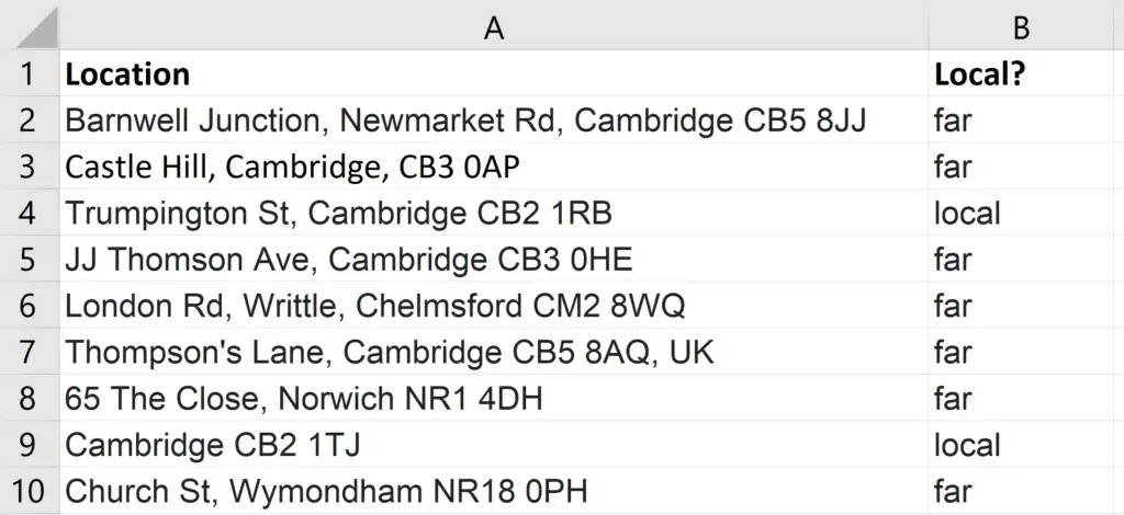
For our example, we have a list of addresses as shown below. And we want to display the word ‘local’ if the address contains the text ‘CB2’.
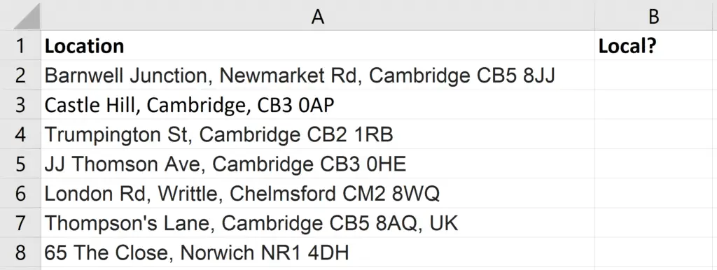
So any postcode beginning with ‘CB2’ is considered local. Anything else is not.
Watch the Video – IF Function Contains Text Match
Check If Cell Contains Text
As mentioned, the IF function always performs an exact match. Therefore we need a different function to determine if the text is in the cell or not.
The function we will use is SEARCH. This function will return the position of the text inside the cell, if it is present.
=SEARCH("CB2 ",A2)
You have to be careful when testing for partial matches. And in this example a space is added after CB2 in the string to search for. This is done to prevent it finding matches for postcodes such as CB25 or CB22.
There is also a function called FIND which could be used instead of SEARCH. The key difference between the two is that FIND is case sensitive, and SEARCH is not.
Now this function returns the position of the text if found. We are not interested in this, and simply want to know if it exists.
So we will surround the SEARCH function with ISNUMBER to return TRUE if the text is found, and otherwise return FALSE.
=ISNUMBER(SEARCH("CB2 ",A2))
We can now finally add the IF function to display the word ‘local’ if ISNUMBER reports TRUE, and the word ‘far’ if FALSE is returned.
=IF(ISNUMBER(SEARCH("CB2 ",A2)),"local","far")
How about Searching for Two Pieces of Text
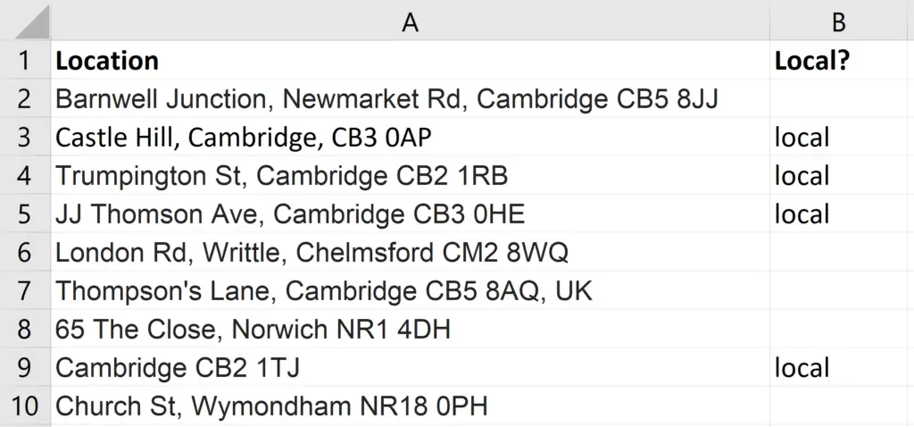
Lets take it a step further. And what if we consider an address to be local if it contains the text ‘CB2’ or ‘CB3’.
We will bring in the OR function for this. A function that can test multiple conditions and returns TRUE if any one of its tests are met.
The formula below can be used. This time the cell is made blank if it is not local.
=IF(OR(ISNUMBER(SEARCH("CB2 ",A2)),ISNUMBER(SEARCH("CB3 ",A2))),"local","")
Reader Interactions
To search a string for a matching word from another string, we use the «IF», «ISNUMBER», «FIND» and «LEFT» functions in Microsoft Excel 2010.
IF: — Checks whether a condition is met and returns one value if True and another value if False.
Syntax of “IF” function =if(logical test,[value_if_true],[value_if_false])
The logical test is performed and if true, the value_if_true output is given, else the output in the value_if_false parameter is given.
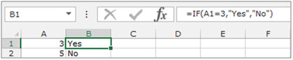
For example:Cells A2 and A3 contain the numbers 3 and 5. If the number in the cell is 3, then the formula should display “Yes”, else “No”.
=IF (A1=3,»Yes»,»No»)
ISNUMBER: — In Microsoft Excel, “ISNUMBER” function is used to check if the value in the cell contains a number or not.
Syntax of “ISNUMBER” function: =ISNUMBER (value)
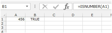
Example:Cell A2 contains the number456
=ISNUMBER (A2), function will return true
FIND:This function returns the location number of the character at which a specific character or text string is first found, reading left to right (not case-sensitive).
Syntax of “FIND” function: =FIND (find_text,within_text,[start_num])
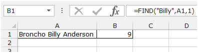
Example:Cell A1contains the text “Broncho Billy Anderson”
=FIND («Billy», A1, 1), function will return 9
LEFT: Returns the specified number of characters starting from the left-most character in the string.
Syntax of “LEFT” function: =LEFT (text,[num_chars])
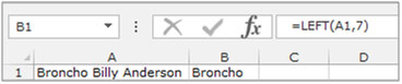
Example:Cell A1contains the text “Broncho Billy Anderson”
=LEFT (A1, 7), function will return “Broncho”
Let’s take an example to understand how we can search the string for a matching word from another string.
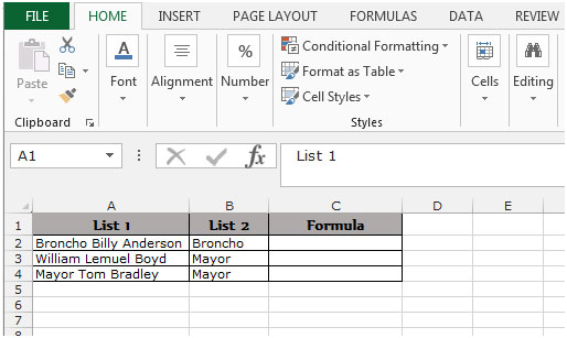
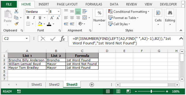
Example 1: We have 2 lists,in column A and column B. Weneed to match the first word in each cell in column A with column B.
Follow the below given steps:-
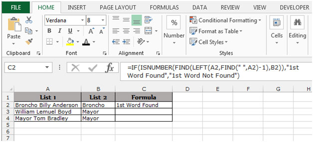
- Select the cell C2, write the formula
- =IF(ISNUMBER(FIND(LEFT(A3,FIND(» «,A3)-1),B3)),»1st Word Found»,»1st Word Not Found»)
- Press Enter on your keyboard.
- The function will search a string for a matching word from another string. It will compare the string in List 2 with List 1 and if found, it will return “1st Word Found”, else it will return “1st Word Not Found”.
- To copy the formula in all cells, press the key “CTRL + C” and select the cell C3:C4 and press the key “CTRL + V” on your keyboard.
This is how we can search a string for a matching word from another string in Microsoft Excel.
Explanation
This formula uses two named ranges: things, and results. If you are porting this formula directly, be sure to use named ranges with the same names (defined based on your data). If you don’t want to use named ranges, use absolute references instead.
The core of this formula is this snippet:
ISNUMBER(SEARCH(things,B5)
This is based on another formula (explained in detail here) that checks a cell for a single substring. If the cell contains the substring, the formula returns TRUE. If not, the formula returns FALSE.
Because we are giving the SEARCH function more than one thing to look for, in the named range things, it will give us more the one result, in an array that looks like this:
{#VALUE!;9;#VALUE!;#VALUE!}
Numbers represent matches in things, errors represent items that were not found.
To simplify the array, we use the ISNUMBER function to convert all items in the array to either TRUE or FALSE. Any valid number becomes TRUE, and any error (i.e. a thing not found) becomes FALSE. The result is an array like this:
{FALSE;TRUE;FALSE;FALSE}
which goes into the MATCH function as the lookup_array argument, with a lookup_value of TRUE:
MATCH(TRUE,{FALSE;TRUE;FALSE;FALSE},0) // returns 2
MATCH then returns the position of first TRUE found, 2 in this case.
Finally, we use the INDEX function to retrieve a result from the named range results at that same position:
=INDEX(results,2) // returns "found red"
You can customize the results range with whatever values make sense in your use case.
Preventing false matches
One problem with this approach with the ISNUMBER + SEARCH approach is you may get false matches from partial matches inside longer words. For example, if you try to match «dr» you may also find «Andrea», «drank», «drip», etc. since «dr» appears inside these words. This happens because SEARCH automatically does a «contains-type» match.
For a quick fix, you can wrap search words in space characters (i.e. » dr «, or «dr «) to avoid finding «dr» in another word. But this will fail if «dr» appears first or last in a cell.
If you need a more robust solution, one option is to normalize the text first in a helper column, and add a leading and trailing space. Then use the formula on this page on the text in the helper column, instead of the original text.
Author: Oscar Cronquist Article last updated on February 01, 2023
This article demonstrates several ways to check if a cell contains any value based on a list. The first example shows how to check if any of the values in the list is in the cell.
The remaining examples show formulas that also return the matching values. You may need different formulas based on the Excel version you are using.
Read this article If cell equals value from list to match the entire cell to any value from a list. To match a single cell to a single value read this: If cell contains text
To check if a cell contains all values in the list read this: If cell contains multiple values
What’s on this page
- Check if the cell contains any value in the list
- Display matches if cell contains text from list (Excel 2019)
- Display matches if cell contains text from list (Earlier Excel versions)
- Filter delimited values not in list (Excel 365)
1. Check if the cell contains any value in the list
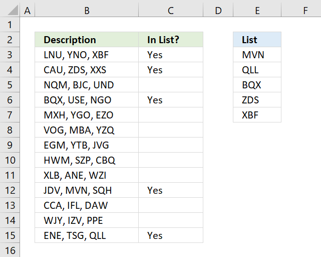
The image above shows an array formula in cell C3 that checks if cell B3 contains at least one of the values in List (E3:E7), it returns «Yes» if any of the values are found in column B and returns nothing if the cell contains none of the values.
For example, cell B3 contains XBF which is found in cell E7. Cell B4 contains text ZDS found in cell E6. Cell C5 contains no values in the list.
=IF(OR(COUNTIF(B3,»*»&$E$3:$E$7&»*»)), «Yes», «»)
You need to enter this formula as an array formula if you are not an Excel 365 subscriber. There is another formula below that doesn’t need to be entered as an array formula, however, it is slightly larger and more complicated.
- Type formula in cell C3.
- Press and hold CTRL + SHIFT simultaneously.
- Press Enter once.
- Release all keys.
Excel adds curly brackets to the formula automatically if you successfully entered the array formula. Don’t enter the curly brackets yourself.
Back to top
1.1 Explaining formula in cell C3
Step 1 — Check if the cell contains any of the values in the list
The COUNTIF function lets you count cells based on a condition, however, it also allows you to count cells based on multiple conditions if you use a cell range instead of a cell.
COUNTIF(range, criteria)
The criteria argument utilizes a beginning and ending asterisk in order to match a text string and not the entire cell value, asterisks are one of two wildcard characters that you are allowed to use.
The ampersands concatenate the asterisks to cell range E3:E7.
COUNTIF(B3,»*»&$E$3:$E$7&»*»)
becomes
COUNTIF(«LNU, YNO, XBF», {«*MVN*»; «*QLL*»; «*BQX*»; «*ZDS*»; «*XBF*»})
and returns this array
{0; 0; 0; 0; 1}
which tells us that the last value in the list is found in cell B3.
Step 2 — Return TRUE if at least one value is 1
The OR function returns TRUE if at least one of the values in the array is TRUE, the numerical equivalent to TRUE is 1.
OR({0; 0; 0; 0; 1})
returns TRUE.
Step 3 — Return Yes or nothing
The IF function then returns «Yes» if the logical test evaluates to TRUE and nothing if the logical test returns FALSE.
IF(TRUE, «Yes», «»)
returns «Yes» in cell B3.
Back to top
Regular formula
The following formula is quite similar to the formula above except that it is a regular formula and it has an additional INDEX function.
=IF(OR(INDEX(COUNTIF(B3,»*»&$E$3:$E$7&»*»),)), «Yes», «»)
Back to top
Back to top
2. Display matches if the cell contains text from a list

The image above demonstrates a formula that checks if a cell contains a value in the list and then returns that value. If multiple values match then all matching values in the list are displayed.
For example, cell B3 contains «ZDS, YNO, XBF» and cell range E3:E7 has two values that match, «ZDS» and «XBF».
Formula in cell C3:
=TEXTJOIN(«, «, TRUE, IF(COUNTIF(B3, «*»&$E$3:$E$7&»*»), $E$3:$E$7, «»))
The TEXTJOIN function is available for Office 2019 and Office 365 subscribers. You will get a #NAME error if your Excel version is missing this function. Office 2019 users may need to enter this formula as an array formula.
The next formula works with most Excel versions.
Array formula in cell C3:
=INDEX($E$3:$E$7, MATCH(1, COUNTIF(B3, «*»&$E$3:$E$7&»*»), 0))
However, it only returns the first match. There is another formula below that returns all matching values, check it out.
How to enter an array formula
Back to top
2.1 Explaining formula in cell C3
Step 1 — Count cells containing text strings
The COUNTIF function lets you count cells based on a condition, we are going to use multiple conditions. I am going to use asterisks to make the COUNTIF function check for a partial match.
The asterisk is one of two wild card characters that you can use, it matches 0 (zero) to any number of any characters.
COUNTIF(B3, «*»&$E$3:$E$7&»*»)
becomes
COUNTIF(«ZDS, YNO, XBF», {«*MVN*»; «*QLL*»; «*BQX*»; «*ZDS*»; «*XBF*»})
and returns {1; 0; 0; 0; 1}.
This array contains as many values as there values in the list, the position of each value in the array matches the position of the value in the list. This means that we can tell from the array that the first value and the last value is found in cell B3.
Step 2 — Return the actual value
The IF function returns one value if the logical test is TRUE and another value if the logical test is FALSE.
IF(logical_test, [value_if_true], [value_if_false])
This allows us to create an array containing values that exists in cell B3.
IF(COUNTIF(B3, «*»&$E$3:$E$7&»*»), $E$3:$E$7, «»)
becomes
IF(COUNTIF(«ZDS, YNO, XBF», {«*MVN*»; «*QLL*»; «*BQX*»; «*ZDS*»; «*XBF*»}), {«*MVN*»; «*QLL*»; «*BQX*»; «*ZDS*»; «*XBF*»}, «»)
and returns {«»;»»;»»;»ZDS»;»XBF»}.
Step 3 — Concatenate values in array
The TEXTJOIN function allows you to combine text strings from multiple cell ranges and also use delimiting characters if you want.
TEXTJOIN(delimiter, ignore_empty, text1, [text2], …)
TEXTJOIN(«, «, TRUE, IF(COUNTIF(B3, «*»&$E$3:$E$7&»*»), $E$3:$E$7, «»))
becomes
TEXTJOIN(«, «, TRUE, {«»;»»;»»;»ZDS»;»XBF»})
and returns text strings ZDS, XBF.
Back to top
3. Display matches if cell contains text from a list (Earlier Excel versions)

The image above demonstrates a formula that returns multiple matches if the cell contains values from a list. This array formula works with most Excel versions.
Array formula in cell C3:
=IFERROR(INDEX($G$3:$G$7, SMALL(IF(COUNTIF($B3, «*»&$G$3:$G$7&»*»), MATCH(ROW($G$3:$G$7), ROW($G$3:$G$7)), «»), COLUMNS($A$1:A1))), «»)
How to enter an array formula
Copy cell C3 and paste to cell range C3:E15.
Back to top
3.1 Explaining formula in cell C3
Step 1 — Identify matching values in cell
The COUNTIF function lets you count cells based on a condition, we are going to use a cell range instead. This will return an array of values.
COUNTIF($B3, «*»&$G$3:$G$7&»*»)
becomes
COUNTIF(«ZDS, YNO, XBF», {«*MVN*»; «*QLL*»; «*BQX*»; «*ZDS*»; «*XBF*»})
and returns {0; 0; 0; 1; 1}.
Step 2 — Calculate relative positions of matching values
The IF function returns one value if the logical test is TRUE and another value if the logical test is FALSE.
IF(logical_test, [value_if_true], [value_if_false])
This allows us to create an array containing values representing row numbers.
IF(COUNTIF($B3, «*»&$G$3:$G$7&»*»), MATCH(ROW($G$3:$G$7), ROW($G$3:$G$7)), «»)
becomes
IF({0; 0; 0; 2; 1}, MATCH(ROW($G$3:$G$7), ROW($G$3:$G$7)), «»)
becomes
IF({0; 0; 0; 2; 1}, {1; 2; 3; 4; 5}, «»)
and returns {«»; «»; «»; 4; 5}.
Step 3 — Extract the k-th smallest number
I am going to use the SMALL function to be able to extract one value in each cell in the next step.
SMALL(array, k)
SMALL(IF(COUNTIF($B3, «*»&$G$3:$G$7&»*»), MATCH(ROW($G$3:$G$7), ROW($G$3:$G$7)), «»), COLUMNS($A$1:A1)))
becomes
SMALL({«»; «»; «»; 4; 5}, COLUMNS($A$1:A1)))
The COLUMNS function calculates the number of columns in a cell range, however, the cell reference in our formula grows when you copy the cell and paste to adjacent cells to the right.
SMALL({0; 0; 0; 4; 5}, COLUMNS($A$1:A1)))
becomes
SMALL({«»; «»; «»; 4; 5}, 1)
and returns 4.
Step 4 — Return value based on row number
The INDEX function returns a value from a cell range or array, you specify which value based on a row and column number. Both the [row_num] and [column_num] are optional.
INDEX(array, [row_num], [column_num])
INDEX($G$3:$G$7, SMALL(IF(COUNTIF($B3, «*»&$G$3:$G$7&»*»), MATCH(ROW($G$3:$G$7), ROW($G$3:$G$7)), «»), COLUMNS($A$1:A1)))
becomes
INDEX($G$3:$G$7, 4)
becomes
INDEX({«MVN»;»QLL»;»BQX»;»ZDS»;»XBF»}, 4)
and returns «ZDS» in cell C3.
Step 5 — Remove error values
The IFERROR function lets you catch most errors in Excel formulas except #SPILL! errors. Be careful when using the IFERROR function, it may make it much harder spotting formula errors.
IFERROR(value, value_if_error)
There are two arguments in the IFERROR function. The value argument is returned if it is not evaluating to an error. The value_if_error argument is returned if the value argument returns an error.
IFERROR(INDEX($G$3:$G$7, SMALL(IF(COUNTIF($B3, «*»&$G$3:$G$7&»*»), MATCH(ROW($G$3:$G$7), ROW($G$3:$G$7)), «»), COLUMNS($A$1:A1))), «»)
Back to top
4. Filter delimited values not in the list (Excel 365)

The formula in cell C3 lists values in cell B3 that are not in the List specified in cell range E3:E7. The formula returns #CALC! error if all values are in the list, see cell C14 as an example.
Excel 365 dynamic array formula in cell C3:
=LET(z,TRIM(TEXTSPLIT(B3,,»,»)),TEXTJOIN(«, «,TRUE,FILTER(z,NOT(COUNTIF($E$3:$E$7,z)))))
4.1 Explaining formula
Step 1 — Split values with a delimiting character
The TEXTSPLIT function splits a string into an array based on delimiting values.
Function syntax: TEXTSPLIT(Input_Text, col_delimiter, [row_delimiter], [Ignore_Empty])
TEXTSPLIT(B3,,»,»)
becomes
TEXTSPLIT(«ZDS, VTO, XBF»,,»,»)
and returns
{«ZDS»; » VTO»; » XBF»}
Step 2 — Remove leading and trailing spaces
The TRIM function deletes all blanks or space characters except single blanks between words in a cell value.
Function syntax: TRIM(text)
TRIM(TEXTSPLIT(B3,,»,»))
becomes
TRIM({«ZDS»; » VTO»; » XBF»})
and returns
{«ZDS»; «VTO»; «XBF»}
Step 3 — Check if values are in list
The COUNTIF function calculates the number of cells that is equal to a condition.
Function syntax: COUNTIF(range, criteria)
COUNTIF($E$3:$E$7,TRIM(TEXTSPLIT(B3,,»,»)))
becomes
COUNTIF({«MVN»;»QLL»;»BQX»;»ZDS»;»XBF»},{«ZDS»; «VTO»; «XBF»})
and returns
{1; 0; 1}
These numbers indicate if a value is found in the list, zero means not in the list and 1 or higher means that the value is in the list at least once.
The number’s position corresponds to the position of the values. {1; 0; 1} — {«ZDS»; «VTO»; «XBF»} meaning «ZDS» and «XBF» are in the list and «VTO» not.
Step 4 — Not
The NOT function returns the boolean opposite to the given argument.
Function syntax: NOT(logical)
NOT(COUNTIF($E$3:$E$7,TRIM(TEXTSPLIT(B3,,»,»))))
becomes
NOT({1; 0; 1})
and returns
{FALSE; TRUE; FALSE}.
0 (zero) is equivalent to FALSE. The boolean opposite is TRUE.
Any other number than 0 (zero) is equivalent to TRUE. The boolean opposite is FALSE.
Step 5 — Filter
The FILTER function extracts values/rows based on a condition or criteria.
Function syntax: FILTER(array, include, [if_empty])
FILTER(TRIM(TEXTSPLIT(B3,,»,»)),NOT(COUNTIF($E$3:$E$7,TRIM(TEXTSPLIT(B3,,»,»)))))
becomes
FILTER({«ZDS»; «VTO»; «XBF»},{FALSE; TRUE; FALSE})
and returns
«VTO».
Step 6 — Join
The TEXTJOIN function combines text strings from multiple cell ranges.
Function syntax: TEXTJOIN(delimiter, ignore_empty, text1, [text2], …)
TEXTJOIN(«, «,TRUE,FILTER(TRIM(TEXTSPLIT(B3,,»,»)),NOT(COUNTIF($E$3:$E$7,TRIM(TEXTSPLIT(B3,,»,»))))))
becomes
TEXTJOIN(«, «,TRUE,{«VTO»})
and returns
«VTO».
Step 7 — Shorten the formula
The LET function lets you name intermediate calculation results which can shorten formulas considerably and improve performance.
Function syntax: LET(name1, name_value1, calculation_or_name2, [name_value2, calculation_or_name3…])
TEXTJOIN(«, «,TRUE,FILTER(TRIM(TEXTSPLIT(B3,,»,»)),NOT(COUNTIF($E$3:$E$7,TRIM(TEXTSPLIT(B3,,»,»))))))
z — TRIM(TEXTSPLIT(B3,,»,»))
LET(z,TRIM(TEXTSPLIT(B3,,»,»)),TEXTJOIN(«, «,TRUE,FILTER(z,NOT(COUNTIF($E$3:$E$7,z)))))
Back to top