
Explanation
Unlike several other frequently used functions, the IF function does not support wildcards. However, you can use the COUNTIF or COUNTIFS functions inside the logical test of IF for basic wildcard functionality.
In the example shown, the formula in C5 is:
=IF(COUNTIF(B5,"??-????-???"),"","invalid")
Working from the inside out, the logical test inside the IF function is based on the COUNTIF function:
COUNTIF(B5,"??-????-???")
Here, COUNTIF counts cells that match the pattern «??-????-???», but since the range is just one cell, the answer is always 1 or zero. The question mark wildcard (?) means «one character», so COUNTIF returns the number 1 when the text consists of 11 characters with two hyphens, as described by the pattern. If cell contents do not match this pattern, COUNTIF returns zero.
When the count is 1, the IF function returns an empty string («»). When the count is zero, IF returns the text «invalid». This works because of boolean logic, where the number 1 is evaluated as TRUE and the number zero is evaluated as FALSE.
Alternative with SEARCH function
Another way to use wildcards with the IF function is to combine the SEARCH and ISNUMBER functions to create a logical test. This works because the SEARCH function supports wildcards. However, SEARCH and ISNUMBER together automatically perform a «contains-type» match, so wildcards aren’t always needed. This page shows a basic example.
Getting IF Function to Work for Partial Text Match
In the dataset below, we want to write a formula in column B that will search the text in column A. Our formula will search the column A text for the text sequence “AT” and if found display “AT” in column B.

It doesn’t matter where the letters “AT” occur in the column A text, we need to see “AT” in the adjacent cell of column B. If the letters “AT” do not occur in the column A text, the formula in column B should display nothing.
Searching for Text with the IF Function
Let’s begin by selecting cell B5 and entering the following IF formula.
=IF(A5="*AT*","AT","")
Notice the formula returns nothing, even though the text in cell A5 contains the letter sequence “AT”.
The reason it fails is that Excel doesn’t work well when using wildcards directly after an equals sign in a formula.

Any function that uses an equals sign in a logical test does not like to use wildcards in this manner.
“But what about the SUMIFS function?”, I hear you saying.
If you examine a SUMIFS function, the wildcards don’t come directly after the equals sign; they instead come after an argument. As an example:
=SUMIFS($C$4:$C$18,$A$4:$A$18,"*AT*")The wildcard usage does not appear directly after an equals sign.
SEARCH Function to the Rescue
The first thing we need to understand is the syntax of the SEARCH function. The syntax is as follows:
SEARCH(find_text, within_text, [start_num])
- find_text – is a required argument that defines the text you are searching for.
- within_text – is a required argument that defines the text in which you want to search for the value defined in the find_text
- Start_num – is an option argument that defines the character number/position in the within_text argument you wish to start searching. If omitted, the default start character position is 1 (the first character on the left of the text.)
To see if the search function works properly on its own, lets perform a simple test with the following formula.
=SEARCH("AT",A5)
We are returned a character position which the letters “AT” were discovered by the SEARCH function. The first SEARCH found the letters “AT” beginning in the 1st character position of the text. The next discovery was in the 5th character position, and the last discovery was in the 4th character position.
The “#VALUE!” responses are the SEARCH function’s way of letting us know that the letters “AT” were not found in the search text.
We can use this new information to determine if the text “AT” exists in the companion text strings. If we see any number as a response, we know “AT” exists in the text string. If we receive an error response, we know the text “AT” does not exist in the text string.
NOTE: The SEARCH function is NOT case-sensitive. A search for the letters “AT” would find “AT”, “At”, “aT”, and “at”. If you wish to search for text and discriminate between different cases (case-sensitive), use the FIND function. The FIND function works the same as SEARCH, but with the added behavior of case-sensitivity.
Turning Numbers into Decisions
An interesting function in Excel is the ISNUMBER function. The purpose of the ISNUMBER function is to return “True” if something is a number and “False” if something is not a number. The syntax is as follows:
ISNUMBER(value)
- value – is a required argument that defines the data you are examining. The value can refer to a cell, a formula, or a name that refers to a cell, formula, or value.
Let’s add the ISNUMBER function to the logic of our previous SEARCH function.
=ISNUMBER(SEARCH("AT",A5))
Any cell that contained a numeric response is now reading “True” and any cell that contained an error is now reading “False”.
We are now able to use the ISNUMBER/SEARCH functions as our wildcard statement in the original IF function.
=IF(ISNUMBER(SEARCH("AT",A5)),"AT","")
This is a great way to perform logical tests in functions that do not allow for wildcards.
Let’s see another scenario
Suppose we want to search for two different sets of text (“AT” or “DE”) and return the word “Europe” if either of these text strings are discovered in the searched text. We will combine the original formula with an OR function to search for multiple text strings.
=IF(OR(ISNUMBER(SEARCH("AT",A5)),ISNUMBER(SEARCH("DE",A5))),
"Europe","")
Practice Workbook
Feel free to Download the Workbook HERE.
![]()
Published on: June 2, 2019
Last modified: March 29, 2023


Leila Gharani
I’m a 5x Microsoft MVP with over 15 years of experience implementing and professionals on Management Information Systems of different sizes and nature.
My background is Masters in Economics, Economist, Consultant, Oracle HFM Accounting Systems Expert, SAP BW Project Manager. My passion is teaching, experimenting and sharing. I am also addicted to learning and enjoy taking online courses on a variety of topics.
In this article, we will learn about how to use Wildcards with IF function in Excel.
IF function is logic test excel function. IF function tests a statement and returns values based on the result.
Syntax:
=IF(logic_test, value_if_true, value_if_false)
We will be using the below wildcards in logic test
There are three wildcard characters in Excel
- Question mark (?) : This wildcard is used to search for any single character.
- Asterisk (*): This wildcard is used to find any number of characters preceding or following any character.
- Tilde (~): This wildcard is an escape character, used preceding the question mark (?) or asterisk mark (*).
Not all functions can execute Wildcards with Excel functions.
Here is a list of functions that accepts wildcards.
- AVERAGEIF, AVERAGEIFS
- COUNTIF, COUNTIFS
- SUMIF, SUMIFS
- VLOOKUP, HLOOKUP
- MATCH
- SEARCH
Let’s understand this function using it an example.
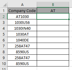
Here we have company codes on one side. And we need to find the fields where phrase AT is present anywhere in the code.
IF function doesn’t support wildcards so we will be using the SEARCH function. SEARCH function returns a number if the phrase is present within the text.
Use the formula:
SEARCH function accepts the wildcard (*) and finds the phrase “AT”, within A2. It returns a number if SEARCH finds the phrase.
ISNUMBER function finds the number and returns TRUE.
IF function logic_test results in TRUE and FALSE and returns “AT” if True or “”(empty string) if False.
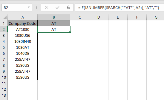
As you can see the formula catches the AT in A2 cell and returns the phrase. This shows A2 cell has “AT” pharse within text.
Now use the formula in other cells to get all fields containing the phrase “AT”.
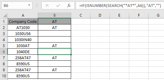
As you can see we used wildcards with IF function to get the result.
Hope you understood how to use in Excel. Explore more articles on Excel cell reference function here. Please feel free to state your query or feedback for the above article.
Related Articles:
How to use the Wildcards in Excel
IF not this or that in Microsoft Excel
IF with OR Function in Excel
Popular Articles:
How to use the VLOOKUP Function in Excel
How to use the COUNTIF function in Excel 2016
How to use the SUMIF Function in Excel
Содержание
- Excel IF Function – How to Use
- Definition of Excel IF Function
- Syntax
- Important Characteristics of IF Function in Excel
- Comparison Operators That Can Be Used With IF Statements
- Example 1: Using ‘equal to’ comparison operator within the IF function
- Example 2: Using ‘not equal to’ comparison operator within the IF function.
- Example 3: Using ‘less than’ operator within the IF function.
- Example 4: Using ‘greater than or equal to’ operator within the IF statement.
- Example 5: Using ‘greater than’ operator within the IF statement.
- Example 6: Using ‘less than or equal to’ operator within the IF statement.
- Example 7: Using an Excel Logical Function within the IF formula in Excel.
- Example 8: Using the Excel IF function to return another formula a result.
- Use Of AND & OR Functions or Logical Operators with Excel IF Statement
- Example 9: Using the IF function along with AND Function.
- Example 10: Using the IF function along with OR Function.
- Nested IF Statements
- Syntax:
- The above syntax translates to this:
- Example 11: Nested IF Statements
- Partial Matching or Wildcards with IF Function
- Example 12: Using FIND and SEARCH functions inside the IF statement
- Example 13: Using SEARCH function inside the Excel IF formula with wildcard operators
- Some Practical Examples of using the IF function
- Example 14: Using Excel IF function with dates.
- Example 15: Use an IF function-based formula to find blank cells in excel.
- Example 16: Use the Excel IF statement to show symbolic results (instead of textual results).
- IFS Function In Excel:
- Syntax for IFS function:
- Example 17: Using IFS function in Excel
- Subscribe and be a part of our 15,000+ member family!
Excel IF Function – How to Use
IF function is undoubtedly one of the most important functions in excel. In general, IF statements give the desired intelligence to a program so that it can make decisions based on given criteria and, most importantly, decide the program flow.
In Microsoft Excel terminology, IF statements are also called «Excel IF-Then statements». IF function evaluates a boolean/logical expression and returns one value if the expression evaluates to ‘TRUE’ and another value if the expression evaluates to ‘FALSE’.
Table of Contents
Definition of Excel IF Function
According to Microsoft Excel, IF function is defined as a formula which «checks whether a condition is met, returns one value if true and another value if false».
Syntax
Syntax of IF function in Excel is as follows:
‘logic_test’ (required argument) – Refers to the boolean expression or logical expression that needs to be evaluated.
‘value_if_true’ (optional argument) – Refers to the value that will be returned by the IF function if the ‘logic_test’ evaluates to TRUE.
‘value_if_false’ (optional argument) – Refers to the value that will be returned by the IF function if the ‘logic_test’ evaluates to FALSE.

Important Characteristics of IF Function in Excel
- To use the IF function, you need to provide the ‘logic_test’ or conditional statement mandatorily.
- The arguments ‘value_if_true’ and ‘value_if_false’ are optional, but you need to provide at least one of them.
- The result of the IF statement can only be any one of the two given values (either it will be ‘value_if_true’ or ‘value_if_false’ ). Both values cannot be returned at the same time.
- IF function throws a ‘#Name?’ error if the ‘logic_test’ or boolean expression you are trying to evaluate is invalid.
- Nesting of IF statements is possible, but Excel only allows this to 64 levels. Nesting of IF statement means using one if statement within another.
Comparison Operators That Can Be Used With IF Statements
Following comparison operators can be used within the ‘logic_test’ argument of the IF function:
- = (equal to)
- <> (not equal to)
- (greater than)
- >= (greater than or equal to)
- Simple Examples of Excel IF Statement
Now, let’s try to see a simple example of the Excel IF function:
Example 1: Using ‘equal to’ comparison operator within the IF function
In this example, we have a list of colors, and we aim to find the ‘Blue’ color. If we are able to find the ‘Blue’ color, then in the adjacent cell, we need to assign a ‘Yes’; otherwise, assign a ‘No’.

So, the formula would be:
This suggests that if the value present in cell A2 is ‘Blue’, then return a ‘Yes’; otherwise, return a ‘No’.
If we drag this formula down to all the rows, we will find that it returns ‘Yes’ for the cells with the value ‘Blue’ for all others; it would result in ‘No’.
Example 2: Using ‘not equal to’ comparison operator within the IF function.
Let’s take example 1, and understand how we can reverse the logic and use a ‘not equal to’ operator to construct the formula so that it still results in ‘Yes’ for ‘Blue’ color and ‘No’ for any other text.

So the formula would be:
This suggests that if the value at A2 is not equal to ‘Blue’, then return a ‘No’; otherwise, return a ‘Yes’.
When dragged down to all the below rows, this formula would find all the cells (from A2 to A8) where the value is not ‘Blue’ and marks a ‘No’ against them. Otherwise, it marks a ‘Yes’ in the adjacent cells.
Example 3: Using ‘less than’ operator within the IF function.
In this example, we have scores of some students, along with their names. We want to assign either «Pass» or «Fail» against each student in the result column.

Based on our criteria, the passing score is 50 or more.
For this, we can use the IF function as:
This suggests that if the value at B2, i.e., 37, is less than 50, then return «Fail»; otherwise, return «Pass».
As 37 is less than 50 so the result will be «Fail».
We can drag the above-given formula for the rest of the cells below and the result would be correct.
Example 4: Using ‘greater than or equal to’ operator within the IF statement.
Let’s take example 3 and see how we can reverse the logic and use a ‘greater than or equal to’ operator to construct the formula so that it still results in ‘Pass’ for scores of 50 or more and ‘Fail’ for all the other scores.

For this, we can use the Excel IF function as:
This suggests that if the value at B2, i.e., 37 is greater than or equal to 50, then return «Pass»; otherwise, return «Fail».
As 37 not greater than or equal to 50 so the result will be «Fail».
When dragged down for the rest of the cells below, this formula would assign the correct result in the adjacent rows.
Example 5: Using ‘greater than’ operator within the IF statement.
In this example, we have a small online store that gives a discount to its customers based on the amount they spend. If a customer spends $50 or more, he is applicable for a 5% discount; otherwise, no discounts are offered.

To find whether a discount is offered or not, we can use the following excel formula:
This translates to – If the value at B2 cell is greater than 50, assign a text «5% Discount» otherwise, assign a text «No Discount» against the customer.
In the first case, as 23 is not greater than 50, the output will be «No Discount».
We can drag the above-given formula for the rest of the cells below are the result would be correct.
Example 6: Using ‘less than or equal to’ operator within the IF statement.
Let’s take example 5 and see how we can reverse the logic and use a ‘less than or equal to’ operator to construct the formula so that it still results in a ‘5% Discount’ for all customers whose total spend exceeds $50 and ‘No Discount’ for all the other customers.

For this, we can use the IF-then statement as:
This means that if the value at B2, i.e., 23, is less than or equal to 50, then return «No Discount»; otherwise, return «5% Discount».
As 23 is less than or equal to 50 so the result will be «No Discount».
When dragged down for the rest of the cells below, this formula would assign the correct result in the adjacent rows.
Example 7: Using an Excel Logical Function within the IF formula in Excel.
In this example, let’s suppose we have a list of numbers, and we have to mark Even and Odd numbers. We can do this using the IF condition and the ISEVEN or ISODD inbuilt functions provided by Microsoft Excel.
ISEVEN function returns ‘true’ if the number passed to it is even; otherwise, it returns a ‘false’. Similarly, ISODD function return ‘true’ if the number passed to it is odd; otherwise, it returns a ‘false’.

For this, we can use the IF-then statement as:
This means that – If the value at A2 cell is an even number, then the result would be «Even»; otherwise, the result would be «Odd».
Alternatively, the above logic can also be written using the ISODD function along with the IF statement as:
This means that – If the value at A2 cell is an odd number, then the result would be «Odd»; otherwise, the result would be «Even».
Example 8: Using the Excel IF function to return another formula a result.
In this example, we have Employee Data from a company. The company comes up with a simple way to reward its loyal employees. They decide to give the employees an annual bonus based on the years spent by the employee within the organization.
Employees with experience of more than 5 years are given 10% of annual salary as a bonus whereas everyone else gets a 5% of annual salary as a bonus.

For this, the excel formula would be:
This means that – if the value at B2 (experience column) is greater than 5, then return a result by calculating 10% of C2 (annual salary column). However, if the logic test is evaluated to false, then return the result by calculating 5% of C2 (annual salary column)
Use Of AND & OR Functions or Logical Operators with Excel IF Statement
Excel IF Statement can also be used along with the other functions like AND, OR, NOT for analyzing complex logic. These functions (AND, OR & NOT) are called logical operators as they are used for connecting two or more logical expressions.
AND Function– AND function returns true when all the conditions inside the AND function evaluate to true. The syntax of AND Function in Excel is:
OR Function– OR function returns true when any one of the conditions inside the OR function evaluates to true. The syntax of OR Function in Excel is:
Example 9: Using the IF function along with AND Function.
In this example, we have Math and science test scores of some students, and we want to assign a ‘Pass’ or ‘Fail’ value against the students based on their scores.
Passing criteria: Students have to get more than 50 marks in Math and more than 70 marks in science to pass the test.

Based on the above conditions, the formula would be:
The formula translates to – if the value at B2 (Math score) is greater than 50 and the value at C2 (Science Score) is greater than 70, then assign the value «Pass»; otherwise, assign the value «Fail».
Example 10: Using the IF function along with OR Function.
In this example, we have two test scores of some students, and we want to assign a ‘Pass’ or ‘Fail’ value against the students based on their scores.
Passing criteria: Students have to clear either one of the two tests with more than 50 marks.

Based on the above conditions, the formula would be:
The formula translates to – if either the value at B2 (Test 1 score) is greater than 50, OR the value at C2 (Test 2 Score) is greater than 50, then assign the value «Pass»; otherwise, assign the value «Fail».
Nested IF Statements
When used alone, IF formula can only result in two outcomes, i.e., True or False. But there are many cases when we want to test multiple outcomes with IF statement.
In such cases, nesting two or more IF Then statements one inside another can be convenient in writing formulas.
Syntax:
The syntax of the Nested IF Then statements is as follows:
‘condition_1’ – Refers to the first logical test or conditional expression that needs to be evaluated by the outer IF function.
‘value_if_true_1’ – Refers to the value that will be returned by the outer IF function if the ‘condition_1’ evaluates to TRUE.
‘condition_2’ – Refers to the second logical test or conditional expression that needs to be evaluated by the inner IF function.
‘value_if_true_2’ – Refers to the value that will be returned by the inner IF function if the ‘condition_2’ evaluates to TRUE.
‘value_if_false_2’ – Refers to the value that will be returned by the inner IF function if the ‘condition_2’ evaluates to FALSE.
The above syntax translates to this:
As we can see, Nested formulas can quickly become complicated so, let’s try to understand how nesting of the IF statement works with an example.
Example 11: Nested IF Statements
In this example, we have a list of countries and their average temperatures in degree Celsius for the month of January. Our goal is to categorize the country based on the temperature range as follows:
Criteria: Temperatures below 20 °C should be marked as «Below Room Temperature», temperatures between 20°C to 25°C should be classified as «Normal Room Temperature», whereas any temperature over 25°C should be marked as «Above Room Temperature».

Based on the above conditions, the formula would be:
The formula translates to – if the value at B2 is less than 20, then the text «Below Room Temperature» is returned from the outer IF block. However, if the value at B2 is greater than or equal to 20, then the inner IF block is evaluated.
Inside the inner IF block, the value at B2 is checked. If the value at B2 is greater than or equal to 20 and less than or equal to 25. Then the inner IF block returns the text «Normal Room Temperature».
However, if the condition inside the inner IF block also evaluates to ‘false’ that means the value at B2 is greater than 25, so the result will be «Above Room Temperature».
Partial Matching or Wildcards with IF Function
Although IF function itself doesn’t accept any wildcard characters like (* or ?) while performing the logic test, thankfully, there are ways to perform partial matching and wildcard searches with the IF function.
To perform partial matching inside the IF function, we can use the FIND (case sensitive) or SEARCH (case insensitive) functions.
Let’s have a look at this with some examples.
Example 12: Using FIND and SEARCH functions inside the IF statement
In this example, we have a list of customers, and we need to find all the customers whose last name is «Flynn». If the customer name contains the text «Flynn», then we need to assign a text «Found» against their names. Otherwise, we need to assign a text «Not Found».

For this, we can make use of the FIND function within the IF function as:
Using the FIND function, we perform a case-sensitive search of the text «Flynn» within the customer name column. If the FIND function is able to find the text «Flynn», it returns a number signifying the position where it found the text.
If the number returned by the FIND function is valid, the ISNUMBER Function returns a value true. Else, it returns false. Based on the ISNUMBER function’s output, the logic test is performed and the appropriate value «Found» or «Not Found» is assigned.
Note: It should be noted that the FIND function performs a case-sensitive search.
This means in the above example if the customer name is entered in lower case (like «sean flynn» then the above function would return not found against them.
To perform a case-insensitive search, we can replace the find function with the search function, and the rest of the formula would be the same.
Example 13: Using SEARCH function inside the Excel IF formula with wildcard operators
In this example, we have the same customer list from example 12, and we need to find all the customers whose name contains «M». If the customer name contains the alphabet «M», we need to assign a text «M Found» against their names. Otherwise, we need to assign a text «M Not Found».

For this, we can use the SEARCH function with a wildcard ‘*’ operator inside the IF function as:
For more details on Search Function and wildcard, operators check out this article – Search Function In Excel
Some Practical Examples of using the IF function
Now, let’s have a look at some more practical examples of the Excel IF Function.
Example 14: Using Excel IF function with dates.
In this example, we have a task list along with the task due dates. Our goal is to show results based on the task due date.
If the task due date was in the past, we need to show «Was due <1,2,3..>day(s) back», if the task due date is today’s date, we need to show «Today» and similarly, if the task due date is in the future then we need to show «Due in <1,2,3..>day(s)»

In Microsoft Excel, we can do this with the help of the IF-then statement and TODAY function, as shown below:
This means that – compare the date present in cell B2 if the date is equal to today’s date show the text «Today». If the date in cell B2 is not equal to today’s date, then the inner IF block checks if the date in B2 is greater than today’s date. If the date in cell B2 is greater than today’s date, that means the date is in the future, so show the text «Due in <1,2,3…>days».
However, if the date in cell B2 is not greater than today’s date, that means the date was in the past; in such a case, show the text «Was due <1,2,3..>day(s) back».
You can also go a step further and apply conditional formatting on the range and highlight all the cells with the text «Today!». This will help you to clearly see
Example 15: Use an IF function-based formula to find blank cells in excel.
In this example, we will use the IF function to find the blank cells in Microsoft Excel. We have a list of customers, and in between the list, some of the cells are blank. We aim to find the blank cells and add the text «blank call found!» against them.

We can do this with the help of the IF function along with the ISBLANK function. The ISBLANK function returns a true if the cell reference passed to it is blank. Otherwise, the ISBLANK function returns false.
Let’s see the formula –
This means that – If the cell at A2 is blank, then the resultant text should be «Blank cell found!», however, if the cell at A2 is not blank, then don’t show any text.
Example 16: Use the Excel IF statement to show symbolic results (instead of textual results).
In this example, we have a list of sales employees of a company along with the number of products sold by the employees in the current month. We want to show an upward arrow symbol (↑) if the employee has done more than 50 sales and a downward arrow symbol (↓) if the employee has made less than 50 sales.

To do this, we can use the formula:
This implies – If the value at B2 is greater than 50, then, as a result, show the content in cell G6 (cell containing upward arrow) and otherwise show the content at G8 (cell containing downward arrow)
If you wonder about the ‘$’ signs used in the formula, you can check out this post – Excel Absolute References . These ‘$’ symbols are used for making excel cell references absolute.
IFS Function In Excel:
IFS Function in Microsoft Excel is a great alternative to nested IF Statements. It is very similar to a switch statement. The IFS function evaluates multiple conditions passed to it and returns the value corresponding to the first condition that evaluates to true.
IFS function is a lot simple to write and read than nested IF statements. IFS function is available in Office 2019 and higher versions.
Syntax for IFS function:
‘test1’ (required argument) – Refers to the first logical test that needs to be evaluated.
‘value1’ (required argument) – Refers to the result to be returned when ‘test1’ evaluates to TRUE.
‘test2’ (optional argument) – Refers to the second logical test that needs to be evaluated
‘value2’ (optional argument) – Refers to the result to be returned when ‘test2’ evaluates to TRUE.
Example 17: Using IFS function in Excel
In this example, we have a list of students, along with their scores, and we need to assign a grade to the students based on the scores.
The grading criteria is as follows – Grade A for a score of 90 or more, Grade B for a score between 80 to 89.99, Grade C for a score between 70 to 79.99, Grade D for a score between 60 to 69.99, Grade E for a score between 60 to 59.99, Grade F for a score lower than 50.

Let’s see how easily write such a complicated formula with the IFS function:
This implies that – If B2 is greater than or equal to 90, return A. Else if B2 is greater than or equal to 80, return B. Else if B2 is greater than or equal to 70, return C. Else if B2 is greater than or equal to 60, return D. Else if B2 is greater than or equal to 50, return E. Else if B2 is less than 50, return F.
If you would try to write the same formula using nested IF statements, see how long and complicated it becomes:
So, this was all about the IF function in excel. If you want to learn more about IF function, I would recommend you to go through this article – VBA IF Statement With Examples
Subscribe and be a part of our 15,000+ member family!
Now subscribe to Excel Trick and get a free copy of our ebook «200+ Excel Shortcuts» (printable format) to catapult your productivity.
Источник
Normally, If you want to write an IF formula for text values in combining with the below two logical operators in excel, such as: “equal to” or “not equal to”.
Table of Contents
- Excel IF function check if a cell contains text(case-insensitive)
- Excel IF function check if a cell contains text (case-sensitive)
- Excel IF function check if part of cell matches specific text
- Excel IF function with Wildcards text value
- Related Formulas
- Related Functions
Excel IF function check if a cell contains text(case-insensitive)
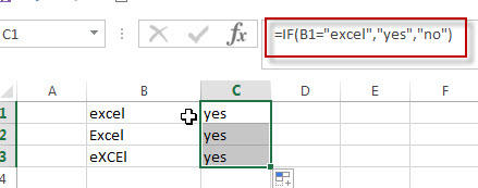
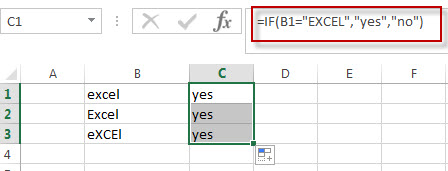
By default, IF function is case-insensitive in excel. It means that the logical text for text values will do not recognize case in the IF formulas. For example, the following two IF formulas will get the same results when checking the text values in cells.
=IF(B1="excel","yes","no")
=IF(B1="EXCEl","yes","no")
The IF formula will check the values of cell B1 if it is equal to “excel” word, If it is TRUE, then return “yes”, otherwise return “no”. And the logical test in the above IF formula will check the text values in the logical_test argument, whatever the logical_test values are “Excel”, “eXcel”, or “EXCEL”, the IF formula don’t care about that if the text values is in lowercase or uppercase, It will get the same results at last.
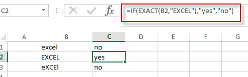
Excel IF function check if a cell contains text (case-sensitive)
If you want to check text values in cells using IF formula in excel (case-sensitive), then you need to create a case-sensitive logical test and then you can use IF function in combination with EXACT function to compare two text values. So if those two text values are exactly the same, then return TRUE. Otherwise return FALSE.
So we can write down the following IF formula combining with EXACT function:
=IF(EXACT(B1,"excel"),"yes","no")
Excel IF function check if part of cell matches specific text
If you want to check if part of text values in cell matches the specific text rather than exact match, to achieve this logic text, you can use IF function in combination with ISNUMBER and SEARCH Function in excel.
Both ISNUMBER and SEARCH functions are case-insensitive in excel.
=IF(ISNUMBER(SEARCH("x",B1)),"good","bad")
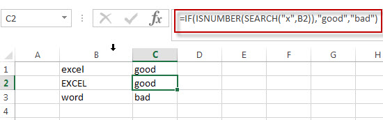
For above the IF formula, it will Check to see if B1 contain the letter x.
Also, we can use FIND function to replace the SEARCH function in the above IF formula. It will return the same results.
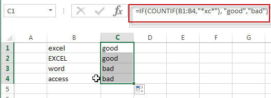
Excel IF function with Wildcards text value
If you wan to use wildcard charcter in an IF formula, for example, if any of the values in column B contains “*xc*”, then return “good”, others return “bad”. You can not directly use the wildcard characters in IF formula, and we can use IF function in combination with COUNTIF function. Let’s see the following IF formula:
=IF(COUNTIF(B1:B4,"*xc*"), "good","bad")
- Excel IF Function With Numbers
If you want to check if a cell values is between two values or checking for the range of numbers or multiple values in cells, at this time, we need to use AND or OR logical function in combination with the logical operator and IF function…
- Excel EXACT function
The Excel SEARCH function returns the number of the starting location of a substring in a text string.The syntax of the EXACT function is as below:= EXACT (text1,text2)… - Excel COUNTIF function
The Excel COUNTIF function will count the number of cells in a range that meet a given criteria.= COUNTIF (range, criteria) … - Excel ISNUMBER function
The Excel ISNUMBER function returns TRUE if the value in a cell is a numeric value, otherwise it will return FALSE. - Excel IF function
The Excel IF function perform a logical test to return one value if the condition is TRUE and return another value if the condition is FALSE…. - Excel SEARCH function
The Excel SEARCH function returns the number of the starting location of a substring in a text string.…
Excel has 3 wildcards you can use in your formulas:
- Asterisk (*) – zero or more characters.
- Question mark (?) – any one character.
- Tilde (~) – escape for literal character (~*) a literal question mark (~?), or a literal tilde (~~).
Contents
- 1 What is wildcard in Excel?
- 2 How do you use wildcard characters?
- 3 How do I use Asterisk in Excel?
- 4 How do I filter wildcards in Excel?
- 5 Why is my wildcard not working Excel?
- 6 How do I find and replace wildcard characters in Excel?
- 7 How do you use wildcards to search files and folders?
- 8 Can you use a wildcard in an Excel IF statement?
- 9 How do I filter special characters in Excel?
- 10 What does * mean in Excel formula?
- 11 How do you do a Vlookup with wildcards in Excel?
- 12 How do you use if and?
- 13 What are wildcards in Windows 10?
- 14 How many wild characters are present for searching files folder?
- 15 How do I search for an exact phrase in Windows 10?
- 16 How do I match a string in Excel?
- 17 How do you match a name in Excel where it is spelling different?
- 18 How do I write regex in Excel?
- 19 How do I get UTF 8 characters in Excel?
- 20 What is the use of * in Excel?
What is wildcard in Excel?
Wildcard characters in Excel are special characters that can be used to take the place of characters in a formula. They are employed in Excel formulas for incomplete matches. Excel supports wildcard characters in formulas to return values that share the same pattern.
How do you use wildcard characters?
The CHARLIST is enclosed in brackets ([ ]) and can be used with wildcard characters for more specific matches.
Examples of wildcard character pattern matching in expressions.
| C haracter(s) | Use to match |
|---|---|
| ? or _ (underscore) | Any single character |
| * or % | Zero or more characters |
How do I use Asterisk in Excel?
The tilde causes Excel to handle the next character literally. In this case we are using “~*” to match a literal asterisk, but this is surrounded by asterisks on either side, in order to match an asterisk anywhere in the cell. If you just want to match an asterisk at the end of a cell, use: “*~*” for the criteria.
How do I filter wildcards in Excel?
#1 Filter Data using Excel Wildcard Characters
- Select the cells that you want to filter.
- Go to Data –> Sort and Filter –> Filter (Keyboard Shortcut – Control + Shift + L).
- Click on the filter icon in the header cell.
- In the field (below the Text Filter option), type A*
- Click OK.
Why is my wildcard not working Excel?
Make sure your data doesn’t contain erroneous characters. When counting text values, make sure the data doesn’t contain leading spaces, trailing spaces, inconsistent use of straight and curly quotation marks, or nonprinting characters. In these cases, COUNTIF might return an unexpected value.
How do I find and replace wildcard characters in Excel?
Replacing a wildcard character
- Press Ctrl + H to open the Find and Replace window.
- Press Replace.
- If we didn’t use tilde and asterisk (~*), just asterisk (*) the result would be like this.
- Excel would treat asterisk as any number of characters (all the text in a cell) and convert it to a word in replace with.
How do you use wildcards to search files and folders?
You can use your own wildcards to limit search results. You can use a question mark (?) as a wildcard for a single character and an asterisk (*) as a wildcard for any number of characters. For example, *. pdf would return only files with the PDF extension.
Can you use a wildcard in an Excel IF statement?
Unlike several other frequently used functions, the IF function does not support wildcards. However, you can use the COUNTIF or COUNTIFS functions inside the logical test of IF for basic wildcard functionality.
How do I filter special characters in Excel?
Re: how to filter special characters in Excel
You can use ‘custom filter’ option available in filter option to find text with special characters. You just need to place ~ before the special character you want to filter.
What does * mean in Excel formula?
In Excel formula, the symbol “*” means multiplication. Say cell A1 contains 5 and cell A2 contains 8.
How do you do a Vlookup with wildcards in Excel?
To use wildcards with VLOOKUP, you must specify exact match mode by providing FALSE or 0 (zero) for the last argument called range_lookup. This expression joins the text in the named range value with a wildcard using the ampersand (&) to concatenate.
How do you use if and?
When you combine each one of them with an IF statement, they read like this:
- AND – =IF(AND(Something is True, Something else is True), Value if True, Value if False)
- OR – =IF(OR(Something is True, Something else is True), Value if True, Value if False)
- NOT – =IF(NOT(Something is True), Value if True, Value if False)
What are wildcards in Windows 10?
The asterisk (*) and question mark (?) are used as wildcard characters, as they are in MS-DOS and Windows. The asterisk matches any sequence of characters, whereas the question mark matches any single character.
How many wild characters are present for searching files folder?
There are two wildcard characters: asterisk (*) and question mark (?). Asterisk (*) – Use the asterisk as a substitute for zero or more characters. e.g., friend* will locate all files and folders that begin with friend. Question mark (?)- Use the question mark as a substitute for a single character in a file name.
How do I search for an exact phrase in Windows 10?
To be able to locate exact phrases, you can try entering the phrase twice in quotes. For example, type “search windows” “search windows” to get all the files containing the phrase search windows. Typing “search windows” will only give you all the files containing search or windows.
How do I match a string in Excel?
Compare two strings
- =A1=A2 // returns TRUE.
- =EXACT(A1,A2) // returns FALSE.
- =IF(EXACT(A2,A2),”Yes”,”No”)
How do you match a name in Excel where it is spelling different?
To match spelling different names, you can use the basic not equal sign ‘<>‘.
- First, select the cell where you want to show the spelling differs names.
- Here, I selected the H5 cell to place the result.
- Now, you can write the formula in the formula bar or into your selected cell.
- Type the formula. =B5<>E5.
How do I write regex in Excel?
The methods we can use are:
- Test – check if the pattern can be found in the string. Returns True if it is found, False if it isn’t.
- Execute – returns occurrences of the pattern matched against the string.
- Replace – replaces occurrences of the pattern in the string.
How do I get UTF 8 characters in Excel?
View Unicode characters in Excel:
- Open Excel from your menu or Desktop.
- Navigate to Data → Get External Data → From Text.
- Navigate to the location of the CSV file you want to import.
- Choose the Delimited option.
- Set the character encoding File Origin to 65001: Unicode (UTF-8) from the drop-down list.
What is the use of * in Excel?
Example
| Data | |
|---|---|
| Formula | Description |
| =PRODUCT(A2:A4) | Multiplies the numbers in cells A2 through A4. |
| =PRODUCT(A2:A4, 2) | Multiplies the numbers in cells A2 through A4, and then multiplies that result by 2. |
| =A2*A3*A4 | Multiplies the numbers in cells A2 through A4 by using mathematical operators instead of the PRODUCT function. |
Wildcard is a term for a special kind of a character that can represent one or more «unknown» characters, and Excel has a wildcard character support. You can use wildcards for filtering, searching, or inside the formulas. In this guide, we’re going to show you how to use Excel Wildcard characters for setting up formula criteria.
Download Workbook
Excel wildcard characters
Excel supports 3 kinds of wildcard characters:
| Asterisk (*) | Any value of zero or more |
| Question mark (?) | Any single character |
| Tilde (~) |
Escape for an actual question mark, asterisk, or tilde character.
|
You can use these characters to generate a text pattern for strings that are to be matched. Please note that wildcard characters only work with texts, and do not work with numbers.
Let’s look at some examples:
| Pattern | Meaning | Sample |
| ? | Any one character | «A», «a», «1», «-«, etc. |
| ?? | Any two characters | «A1», «9a», «9.», etc. |
| * | Any characters | «excel», «supp0rtz», «wi!d cards», etc. |
| A* | Starts with «A» | «A», «Anchor», «A string», etc. |
| ?* | At least one character | «Z», «1», «Z1», etc. |
| (???) ???-???? | 10 characters with parenthesis and a hyphen | «(123) 456-7890», «(A10) XYZ-8866», etc. |
| *lec* | Contains «lec» | «electric», dialectic», «lecture», etc. |
| *~? | Ends with a question mark (?) | «O Brother, Where Art Thou?», » Dude, Where’s My Car?», etc. |
Formulas that support using wildcard criteria
All …IFS and …IF Functions
All statistical functions in Excel that end with either «IFS» or «IF» support wildcards.
- SUMIFS
- SUMIF
- COUNTIFS
- COUNTIF
- AVERAGEIFS
- AVERAGEIF
- MAXIFS
- MINIFS
Using wildcard criteria can increase the versatility of these functions. Use strings with wildcards in criteria arguments. The following examples show the difference between using and not using wildcards.

The upper set of formulas are using the «*FIRE*» string which represents any text that contains «FIRE». Thus, the formulas calculates 3 rows of data: «FIRE», «FIRE» and «FIRE, FLYING».
On the other hand, the formulas work on only two of examples without any wildcards: «FIRE» and «FIRE».
VLOOKUP and HLOOKUP
Both VLOOKUP and HLOOKUP functions support wildcard characters. Although both functions have an approximate match mode, using them in this mode may not return the correct result every time. Wildcards gives you more precision on your search. Use a string with a wildcard for lookup value argument to search.
The following screenshot shows an example for each formula. VLOOKUP function searches the «C*n» value, and matches with «Charmeleon». On the other side, HLOOKUP function searches a two-character string that matches «HP».

MATCH
MATCH function is another lookup function that support wildcard characters. Aside from returning a value on a different column, MATCH function returns the position of the found value. Once again, use wildcard characters in the lookup value argument.

SEARCH
You can use the SEARCH function with wildcards to find a string pattern in another string. In our example, we searched for a pattern like «a?to*e» to locate a string starts with «a», followed by any single character, which is followed by «to», and any number of characters until an «e» character is found.

Watch Video on Excel Wildcard Characters
There are only 3 Excel wildcard characters (asterisk, question mark, and tilde) and a lot can be done using these.
In this tutorial, I will show you four examples where these Excel wildcard characters are absolute lifesavers.
Excel Wildcard Characters – An Introduction
Wildcards are special characters that can take any place of any character (hence the name – wildcard).
There are three wildcard characters in Excel:
- * (asterisk) – It represents any number of characters. For example, Ex* could mean Excel, Excels, Example, Expert, etc.
- ? (question mark) – It represents one single character. For example, Tr?mp could mean Trump or Tramp.
- ~ (tilde) – It is used to identify a wildcard character (~, *, ?) in the text. For example, let’s say you want to find the exact phrase Excel* in a list. If you use Excel* as the search string, it would give you any word that has Excel at the beginning followed by any number of characters (such as Excel, Excels, Excellent). To specifically look for excel*, we need to use ~. So our search string would be excel~*. Here, the presence of ~ ensures that excel reads the following character as is, and not as a wildcard.
Note: I have not come across many situations where you need to use ~. Nevertheless, it is a good to know feature.
Now let’s go through four awesome examples where wildcard characters do all the heavy lifting.
Now let’s look at four practical examples where Excel wildcard characters can be mighty useful:
- Filtering data using a wildcard character.
- Partial Lookup using wildcard character and VLOOKUP.
- Find and Replace Partial Matches.
- Count Non-blank cells that contain text.
#1 Filter Data using Excel Wildcard Characters
Excel wildcard characters come in handy when you have huge data sets and you want to filter data based on a condition.
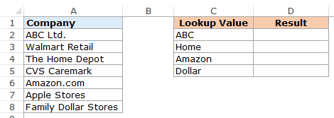
Suppose you have a dataset as shown below:

You can use the asterisk (*) wildcard character in data filter to get a list of companies that start with the alphabet A.
Here is how to do this:
This will instantly filter the results and give you 3 names – ABC Ltd., Amazon.com, and Apple Stores.

How does it work? – When you add an asterisk (*) after A, Excel would filter anything that starts with A. This is because an asterisk (being an Excel wildcard character) can represent any number of characters.
Now with the same methodology, you can use various criteria to filter results.
For example, if you want to filter companies that begin with the alphabet A and contain the alphabet C in it, use the string A*C. This will give you only 2 results – ABC Ltd. and Amazon.com.
If you use A?C instead, you will only get ABC Ltd as the result (as only one character is allowed between ‘a’ and ‘c’)
Note: The same concept can also be applied when using Excel Advanced Filters.
#2 Partial Lookup Using Wildcard Characters & VLOOKUP
Partial look-up is needed when you have to look for a value in a list and there isn’t an exact match.
For example, suppose you have a data set as shown below, and you want to look for the company ABC in a list, but the list has ABC Ltd instead of ABC.
You can not use the regular VLOOKUP function in this case as the lookup value does not have an exact match.
If you use VLOOKUP with an approximate match, it will give you the wrong results.
However, you can use a wildcard character within VLOOKUP function to get the right results:
Enter the following formula in cell D2 and drag it for other cells:
=VLOOKUP("*"&C2&"*",$A$2:$A$8,1,FALSE)
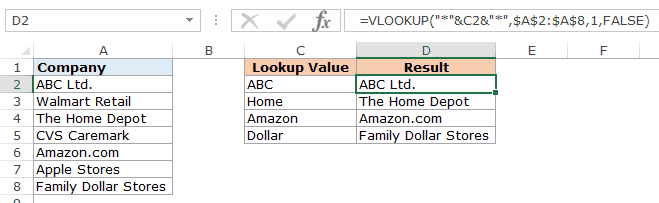
How does this formula work?
In the above formula, instead of using the lookup value as is, it is flanked on both sides with the Excel wildcard character asterisk (*) – “*”&C2&”*”
This tells excel that it needs to look for any text that contains the word in C2. It could have any number of characters before or after the text in C2.
Hence, the formula looks for a match, and as soon as it gets a match, it returns that value.
3. Find and Replace Partial Matches
Excel Wildcard characters are quite versatile.
You can use it in a complex formula as well as in basic functionality such as Find and Replace.
Suppose you have the data as shown below:

In the above data, the region has been entered in different ways (such as North-West, North West, NorthWest).
This is often the case with sales data.
To clean this data and make it consistent, we can use Find and Replace with Excel wildcard characters.
Here is how to do this:
- Select the data where you want to find and replace text.
- Go to Home –> Find & Select –> Go To. This will open the Find and Replace dialogue box. (You can also use the keyboard shortcut – Control + H).
- Enter the following text in the find and replace dialogue box:
- Find what: North*W*
- Replace with: North-West

- Click on Replace All.

This will instantly change all the different formats and make it consistent to North-West.

How does this Work?
In the Find field, we have used North*W* which will find any text that has the word North and contains the alphabet ‘W’ anywhere after it.
Hence, it covers all the scenarios (NorthWest, North West, and North-West).
Find and Replace finds all these instances and changes it to North-West and makes it consistent.
4. Count Non-blank Cells that Contain Text
I know you are smart and you thinking that Excel already has an inbuilt function to do this.
You’re absolutely right!!
This can be done using the COUNTA function.
BUT… There is one small problem with it.
A lot of times when you import data or use other people’s worksheet, you will notice that there are empty cells while that might not be the case.
These cells look blank but have =”” in it. The trouble is that the
The trouble is that the COUNTA function does not consider this as an empty cell (it counts it as text).
See the example below:

In the above example, I use the COUNTA function to find cells that are not empty and it returns 11 and not 10 (but you can clearly see only 10 cells have text).
The reason, as I mentioned, is that it doesn’t consider A11 as empty (while it should).
But that is how Excel works.
The fix is to use the Excel wildcard character within the formula.
Below is a formula using the COUNTIF function that only counts cells that have text in it:
=COUNTIF(A1:A11,"?*")
This formula tells excel to count only if the cell has at least one character.
In the ?* combo:
- ? (question mark) ensures that at least one character is present.
- * (asterisk) makes room for any number of additional characters.
Note: The above formula works when only have text values in the cells. If you have a list that has both text as well as numbers, use the following formula:
=COUNTA(A1:A11)-COUNTBLANK(A1:A11)
Similarly, you can use wildcards in a lot of other Excel functions, such as IF(), SUMIF(), AVERAGEIF(), and MATCH().
It’s also interesting to note that while you can use the wildcard characters in the SEARCH function, you can’t use it in FIND function.
Hope these examples give you a flair of the versatility and power of Excel wildcard characters.
If you have any other innovative way to use it, do share it with me in the comments section.
You May Find the Following Excel Tutorials Useful:
- Using COUNTIF and COUNTIFS with Multiple Criteria.
- Creating a Drop Down List in Excel.
- Intersect Operator in Excel
Excel IF statement for partial text match (wildcard)
Details: WebExcel IF AND formula with wildcards When you want to check if a cell contains two or more different substrings, the easiest way … how to use wildcards in excel
› Verified 6 days ago
› Url: Ablebits.com View Details
› Get more: How to use wildcards in excelDetail Excel
IF with wildcards — Excel formula Exceljet
Details: WebAnother way to use wildcards with the IF function is to combine the SEARCH and ISNUMBER functions to create a logical test. This works because the SEARCH … excel if statement with wildcard
› Verified 7 days ago
› Url: Exceljet.net View Details
› Get more: Excel if statement with wildcardDetail Excel
How to Use Wildcard with If Statement in Excel (5 …
Details: WebYou can use the COUNTIF function in the IF statement to use wildcards. The conditional function COUNTIF counts the wildcards and then returns the value for the next step. Follow the below … excel match wildcard
› Verified 4 days ago
› Url: Exceldemy.com View Details
› Get more: Excel match wildcardDetail Excel
Excel Wildcard Exceljet
Details: WebA wildcard is a special character that lets you perform «fuzzy» matching on text in your Excel formulas. For example, this formula: = COUNTIF (B5:B11,»*combo») counts all cells in the range B5:B11 that end with the … excel wildcard number only
› Verified 8 days ago
› Url: Exceljet.net View Details
› Get more: Excel wildcard number onlyDetail Excel
Excel Function to Check IF a Cell Contains Specific Text
Details: WebIf you examine a SUMIFS function, the wildcards don’t come directly after the equals sign; they instead come after an argument. As an example: =SUMIFS ($C$4:$C$18,$A$4:$A$18,”*AT*”) The wildcard … excel search wildcard number
› Verified 9 days ago
› Url: Xelplus.com View Details
› Get more: Excel search wildcard numberDetail Excel
IF function with Wildcards — Excel Tip
Details: WebIF function tests a statement and returns values based on the result. Syntax: = IF (logic_test, value_if_true, value_if_false) We will be using the below wildcards in logic … list of excel wildcard characters
› Verified 3 days ago
› Url: Exceltip.com View Details
› Get more: List of excel wildcard charactersDetail Excel
Using wildcard characters in searches — Microsoft Support
Details: WebUse wildcard characters as comparison criteria for text filters, and when you’re searching and replacing content. These can also be used in Conditional Formatting rules that use … countif with wildcard
› Verified 7 days ago
› Url: Support.microsoft.com View Details
› Get more: Countif with wildcardDetail Excel
Excel formula LIKE, AND, IF, WILDCARDS — Stack Overflow
Details: WebWildcards aren’t recognised with comparison operators like =, for example if you use this formula =A1=»*&*» that will treat the * ‘s as literal asterisks (not wildcards) …
› Verified Just Now
› Url: Stackoverflow.com View Details
› Get more: ExcelDetail Excel
Excel SUM based on Partial Text Match (SUMIFS with …
Details: WebIntroducing Wildcards. Wildcards represent “any characters” and are useful when you want to capture multiple items in a search based on a pattern of characters. …
› Verified 3 days ago
› Url: Xelplus.com View Details
› Get more: ExcelDetail Excel
Wildcard In Excel — Types, Formulas, How to Use * Character?
Details: WebLet us learn the use of wildcard in excel with the below steps. Step 1: Select the range of cells from the range A2:A10. Step 2: Go to the Home tab, and under Conditional …
› Verified 4 days ago
› Url: Excelmojo.com View Details
› Get more: LearnDetail Excel
How to use Wildcard criteria in Excel formulas
Details: WebAll statistical functions in Excel that end with either «IFS» or «IF» support wildcards. SUMIFS SUMIF COUNTIFS COUNTIF AVERAGEIFS AVERAGEIF MAXIFS MINIFS Using wildcard criteria …
› Verified 5 days ago
› Url: Spreadsheetweb.com View Details
› Get more: ExcelDetail Excel
How To Use Wildcards/Partial Match With Excel’s Filter Function
Details: WebBegins With Wildcard Search (Filter Function) To perform a begins with wildcard search (example = Ash*) you will need to rely on the LEFT Excel function. …
› Verified 4 days ago
› Url: Thespreadsheetguru.com View Details
› Get more: ExcelDetail Excel
Excel wildcard: find and replace, filter, use in formulas
Details: WebIt is sometimes stated that wildcards in Excel only work for text values, not numbers. However, this is not exactly true. With the Find and Replace feature as well as …
› Verified 8 days ago
› Url: Ablebits.com View Details
› Get more: ExcelDetail Excel
Filter Data with the Excel FILTER Function and Wildcards Excel
Details: Web👉 linktr.ee/benthompsonukWelcome to our YouTube tutorial on «Filter Data with the Excel FILTER Function and Wildcards«! In this video, we will explore how t
› Verified 3 days ago
› Url: Youtube.com View Details
› Get more: ExcelDetail Excel
How to Count Specific Items in Excel List — Contextures Excel Tips
Details: WebWith the COUNTIF function syntax, there are 2 required arguments: range — cells to check for criteria; criteria — criteria to match — typed in the formula, or refer to a …
› Verified Just Now
› Url: Contextures.com View Details
› Get more: ExcelDetail Excel
Excel IF Function with PARTIAL Text Match (IF with Wildcards)
Details: WebLearn how to combine Excel‘s IF function with wildcards for a partial text match. For example, you’d like to check IF a cell contains a specific word. If yes
› Verified 3 days ago
› Url: Youtube.com View Details
› Get more: LearnDetail Excel
How to use wildcards with the XLOOKUP() function in Excel
Details: WebSelect I4:J4. On the Home tab, click Conditional Formatting in the Styles group and choose New Rule from the resulting dropdown. In the top pane of the resulting …
› Verified 1 days ago
› Url: Techrepublic.com View Details
› Get more: ExcelDetail Excel
Can you use a wildcard in an IF(OR) function?
Details: WebAnother way without using wild card =IF (COUNT (SEARCH ( {«Alpha»,»Beta»,»Delta»,»Gamma»},A2)),TRUE,FALSE) In case you wondered how many …
› Verified 9 days ago
› Url: Mrexcel.com View Details
› Get more: ExcelDetail Excel
IFS with wildcards — Microsoft Community Hub
Details: WebIf function in Excel will not work when using wildcards directly after an equals sign in a formula. There is other way to work around with this method. This …
› Verified 6 days ago
› Url: Techcommunity.microsoft.com View Details
› Get more: ExcelDetail Excel
Guide to 20 Worksheet Functions that Use Wildcards
Details: WebExcel Functions That Use Wildcards. (Use AVERAGEIFS.) Returns the average (arithmetic mean) of all the cells in a range that meet one criteria. Returns the average of …
› Verified Just Now
› Url: Exceluser.com View Details
› Get more: ExcelDetail Excel