
Normally, If you want to write an IF formula for text values in combining with the below two logical operators in excel, such as: “equal to” or “not equal to”.
Table of Contents
- Excel IF function check if a cell contains text(case-insensitive)
- Excel IF function check if a cell contains text (case-sensitive)
- Excel IF function check if part of cell matches specific text
- Excel IF function with Wildcards text value
- Related Formulas
- Related Functions
Excel IF function check if a cell contains text(case-insensitive)
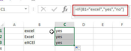
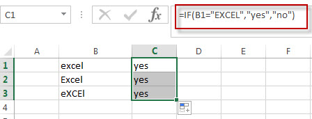
By default, IF function is case-insensitive in excel. It means that the logical text for text values will do not recognize case in the IF formulas. For example, the following two IF formulas will get the same results when checking the text values in cells.
=IF(B1="excel","yes","no")
=IF(B1="EXCEl","yes","no")
The IF formula will check the values of cell B1 if it is equal to “excel” word, If it is TRUE, then return “yes”, otherwise return “no”. And the logical test in the above IF formula will check the text values in the logical_test argument, whatever the logical_test values are “Excel”, “eXcel”, or “EXCEL”, the IF formula don’t care about that if the text values is in lowercase or uppercase, It will get the same results at last.
Excel IF function check if a cell contains text (case-sensitive)
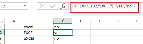
If you want to check text values in cells using IF formula in excel (case-sensitive), then you need to create a case-sensitive logical test and then you can use IF function in combination with EXACT function to compare two text values. So if those two text values are exactly the same, then return TRUE. Otherwise return FALSE.
So we can write down the following IF formula combining with EXACT function:
=IF(EXACT(B1,"excel"),"yes","no")
Excel IF function check if part of cell matches specific text
If you want to check if part of text values in cell matches the specific text rather than exact match, to achieve this logic text, you can use IF function in combination with ISNUMBER and SEARCH Function in excel.
Both ISNUMBER and SEARCH functions are case-insensitive in excel.
=IF(ISNUMBER(SEARCH("x",B1)),"good","bad")
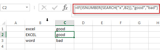
For above the IF formula, it will Check to see if B1 contain the letter x.
Also, we can use FIND function to replace the SEARCH function in the above IF formula. It will return the same results.
Excel IF function with Wildcards text value
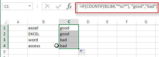
If you wan to use wildcard charcter in an IF formula, for example, if any of the values in column B contains “*xc*”, then return “good”, others return “bad”. You can not directly use the wildcard characters in IF formula, and we can use IF function in combination with COUNTIF function. Let’s see the following IF formula:
=IF(COUNTIF(B1:B4,"*xc*"), "good","bad")
- Excel IF Function With Numbers
If you want to check if a cell values is between two values or checking for the range of numbers or multiple values in cells, at this time, we need to use AND or OR logical function in combination with the logical operator and IF function…
- Excel EXACT function
The Excel SEARCH function returns the number of the starting location of a substring in a text string.The syntax of the EXACT function is as below:= EXACT (text1,text2)… - Excel COUNTIF function
The Excel COUNTIF function will count the number of cells in a range that meet a given criteria.= COUNTIF (range, criteria) … - Excel ISNUMBER function
The Excel ISNUMBER function returns TRUE if the value in a cell is a numeric value, otherwise it will return FALSE. - Excel IF function
The Excel IF function perform a logical test to return one value if the condition is TRUE and return another value if the condition is FALSE…. - Excel SEARCH function
The Excel SEARCH function returns the number of the starting location of a substring in a text string.…
IF function
The IF function is one of the most popular functions in Excel, and it allows you to make logical comparisons between a value and what you expect.
So an IF statement can have two results. The first result is if your comparison is True, the second if your comparison is False.
For example, =IF(C2=”Yes”,1,2) says IF(C2 = Yes, then return a 1, otherwise return a 2).

Use the IF function, one of the logical functions, to return one value if a condition is true and another value if it’s false.
IF(logical_test, value_if_true, [value_if_false])
For example:
-
=IF(A2>B2,»Over Budget»,»OK»)
-
=IF(A2=B2,B4-A4,»»)
|
Argument name |
Description |
|---|---|
|
logical_test (required) |
The condition you want to test. |
|
value_if_true (required) |
The value that you want returned if the result of logical_test is TRUE. |
|
value_if_false (optional) |
The value that you want returned if the result of logical_test is FALSE. |
Simple IF examples

-
=IF(C2=”Yes”,1,2)
In the above example, cell D2 says: IF(C2 = Yes, then return a 1, otherwise return a 2)

-
=IF(C2=1,”Yes”,”No”)
In this example, the formula in cell D2 says: IF(C2 = 1, then return Yes, otherwise return No)As you see, the IF function can be used to evaluate both text and values. It can also be used to evaluate errors. You are not limited to only checking if one thing is equal to another and returning a single result, you can also use mathematical operators and perform additional calculations depending on your criteria. You can also nest multiple IF functions together in order to perform multiple comparisons.

-
=IF(C2>B2,”Over Budget”,”Within Budget”)
In the above example, the IF function in D2 is saying IF(C2 Is Greater Than B2, then return “Over Budget”, otherwise return “Within Budget”)

-
=IF(C2>B2,C2-B2,0)
In the above illustration, instead of returning a text result, we are going to return a mathematical calculation. So the formula in E2 is saying IF(Actual is Greater than Budgeted, then Subtract the Budgeted amount from the Actual amount, otherwise return nothing).

-
=IF(E7=”Yes”,F5*0.0825,0)
In this example, the formula in F7 is saying IF(E7 = “Yes”, then calculate the Total Amount in F5 * 8.25%, otherwise no Sales Tax is due so return 0)
Note: If you are going to use text in formulas, you need to wrap the text in quotes (e.g. “Text”). The only exception to that is using TRUE or FALSE, which Excel automatically understands.
Common problems
|
Problem |
What went wrong |
|---|---|
|
0 (zero) in cell |
There was no argument for either value_if_true or value_if_False arguments. To see the right value returned, add argument text to the two arguments, or add TRUE or FALSE to the argument. |
|
#NAME? in cell |
This usually means that the formula is misspelled. |
Need more help?
You can always ask an expert in the Excel Tech Community or get support in the Answers community.

See Also
IF function — nested formulas and avoiding pitfalls
IFS function
Using IF with AND, OR and NOT functions
COUNTIF function
How to avoid broken formulas
Overview of formulas in Excel
Need more help?
Want more options?
Explore subscription benefits, browse training courses, learn how to secure your device, and more.
Communities help you ask and answer questions, give feedback, and hear from experts with rich knowledge.
You can use the following formulas to use an IF function with text values in Excel:
Method 1: Check if Cell is Equal to Text
=IF(A2="Starting Center", "Yes", "No")
This formula will return “Yes” if the value in cell A2 is “Starting Center” – otherwise it will return “No.”
Method 2: Check if Cell Contains Specific Text
=IF(ISNUMBER(SEARCH("Guard", A2)), "Yes", "No")
This formula will return “Yes” if the value in cell A2 contains “Guard” anywhere in the cell – otherwise it will return “No.”
Method 3: Check if Cell Contains One of Several Specific Texts
=IF(SUMPRODUCT(--ISNUMBER(SEARCH({"Backup","Guard"},A2)))>0, "Yes", "No")
This formula will return “Yes” if the value in cell A2 contains “Backup” or “Guard” anywhere in the cell – otherwise it will return “No.”
The following examples show how to use each formula in practice with the following dataset in Excel:

Example 1: Check if Cell is Equal to Text
We can type the following formula into cell C2 to return “Yes” if the value in cell A2 is equal to “Starting Center” or return “No” otherwise:
=IF(A2="Starting Center", "Yes", "No")
We can then click and drag this formula down to each remaining cell in column C:

The formula returns “Yes” for the one row where the value in column A is equal to “Starting Center” and returns “No” for all other rows.
Example 2: Check if Cell Contains Specific Text
We can type the following formula into cell C2 to return “Yes” if the value in cell A2 contains “Guard” anywhere in the cell or return “No” otherwise:
=IF(ISNUMBER(SEARCH("Guard", A2)), "Yes", "No")
We can then click and drag this formula down to each remaining cell in column C:

The formula returns “Yes” for each row that contains “Guard” in column A and returns “No” for all other rows.
Example 3: Check if Cell Contains Several Specific Texts
We can type the following formula into cell C2 to return “Yes” if the value in cell A2 contains “Backup” or “Guard” anywhere in the cell or return “No” otherwise:
=IF(SUMPRODUCT(--ISNUMBER(SEARCH({"Backup","Guard"},A2)))>0, "Yes", "No")
We can then click and drag this formula down to each remaining cell in column C:

The formula returns “Yes” for each row that contains “Backup” or “Guard” in column A and returns “No” for all other rows.
Note: Feel free to include as many text values as you’d like in the curly brackets in the formula to search for as many specific text values in a cell as you’d like.
Additional Resources
The following tutorials explain how to perform other common tasks in Excel:
Excel: How to Use IF Function with Multiple Conditions
Excel: How to Create IF Function to Return Yes or No
Excel: How to Use an IF Function with Range of Values
Содержание
- IF function
- Simple IF examples
- Common problems
- Need more help?
- Using IF with AND, OR and NOT functions
- Examples
- Using AND, OR and NOT with Conditional Formatting
- Need more help?
- See also
- Функция ЕСЛИ в Excel. Как использовать?
- Что возвращает функция
- Синтаксис
- Аргументы функции
- Дополнительная информация
- Функция Если в Excel примеры с несколькими условиями
- Пример 1. Проверяем простое числовое условие с помощью функции IF (ЕСЛИ)
- Пример 2. Использование вложенной функции IF (ЕСЛИ) для проверки условия выражения
- Пример 3. Вычисляем сумму комиссии с продаж с помощью функции IF (ЕСЛИ) в Excel
- Пример 4. Используем логические операторы (AND/OR) (И/ИЛИ) в функции IF (ЕСЛИ) в Excel
- Пример 5. Преобразуем ошибки в значения “0” с помощью функции IF (ЕСЛИ)
IF function
The IF function is one of the most popular functions in Excel, and it allows you to make logical comparisons between a value and what you expect.
So an IF statement can have two results. The first result is if your comparison is True, the second if your comparison is False.
For example, =IF(C2=”Yes”,1,2) says IF(C2 = Yes, then return a 1, otherwise return a 2).
Use the IF function, one of the logical functions, to return one value if a condition is true and another value if it’s false.
IF(logical_test, value_if_true, [value_if_false])
The condition you want to test.
The value that you want returned if the result of logical_test is TRUE.
The value that you want returned if the result of logical_test is FALSE.
Simple IF examples
In the above example, cell D2 says: IF(C2 = Yes, then return a 1, otherwise return a 2)
In this example, the formula in cell D2 says: IF(C2 = 1, then return Yes, otherwise return No)As you see, the IF function can be used to evaluate both text and values. It can also be used to evaluate errors. You are not limited to only checking if one thing is equal to another and returning a single result, you can also use mathematical operators and perform additional calculations depending on your criteria. You can also nest multiple IF functions together in order to perform multiple comparisons.
B2,”Over Budget”,”Within Budget”)» loading=»lazy»>
=IF(C2>B2,”Over Budget”,”Within Budget”)
In the above example, the IF function in D2 is saying IF(C2 Is Greater Than B2, then return “Over Budget”, otherwise return “Within Budget”)
B2,C2-B2,»»)» loading=»lazy»>
In the above illustration, instead of returning a text result, we are going to return a mathematical calculation. So the formula in E2 is saying IF(Actual is Greater than Budgeted, then Subtract the Budgeted amount from the Actual amount, otherwise return nothing).
In this example, the formula in F7 is saying IF(E7 = “Yes”, then calculate the Total Amount in F5 * 8.25%, otherwise no Sales Tax is due so return 0)
Note: If you are going to use text in formulas, you need to wrap the text in quotes (e.g. “Text”). The only exception to that is using TRUE or FALSE, which Excel automatically understands.
Common problems
What went wrong
There was no argument for either value_if_true or value_if_False arguments. To see the right value returned, add argument text to the two arguments, or add TRUE or FALSE to the argument.
This usually means that the formula is misspelled.
Need more help?
You can always ask an expert in the Excel Tech Community or get support in the Answers community.
Источник
Using IF with AND, OR and NOT functions
The IF function allows you to make a logical comparison between a value and what you expect by testing for a condition and returning a result if that condition is True or False.
=IF(Something is True, then do something, otherwise do something else)
But what if you need to test multiple conditions, where let’s say all conditions need to be True or False ( AND), or only one condition needs to be True or False ( OR), or if you want to check if a condition does NOT meet your criteria? All 3 functions can be used on their own, but it’s much more common to see them paired with IF functions.
Use the IF function along with AND, OR and NOT to perform multiple evaluations if conditions are True or False.
IF(AND()) — IF(AND(logical1, [logical2], . ), value_if_true, [value_if_false]))
IF(OR()) — IF(OR(logical1, [logical2], . ), value_if_true, [value_if_false]))
IF(NOT()) — IF(NOT(logical1), value_if_true, [value_if_false]))
The condition you want to test.
The value that you want returned if the result of logical_test is TRUE.
The value that you want returned if the result of logical_test is FALSE.
Here are overviews of how to structure AND, OR and NOT functions individually. When you combine each one of them with an IF statement, they read like this:
AND – =IF(AND(Something is True, Something else is True), Value if True, Value if False)
OR – =IF(OR(Something is True, Something else is True), Value if True, Value if False)
NOT – =IF(NOT(Something is True), Value if True, Value if False)
Examples
Following are examples of some common nested IF(AND()), IF(OR()) and IF(NOT()) statements. The AND and OR functions can support up to 255 individual conditions, but it’s not good practice to use more than a few because complex, nested formulas can get very difficult to build, test and maintain. The NOT function only takes one condition.

Here are the formulas spelled out according to their logic:
=IF(AND(A2>0,B2 0,B4 50),TRUE,FALSE)
IF A6 (25) is NOT greater than 50, then return TRUE, otherwise return FALSE. In this case 25 is not greater than 50, so the formula returns TRUE.
IF A7 (“Blue”) is NOT equal to “Red”, then return TRUE, otherwise return FALSE.
Note that all of the examples have a closing parenthesis after their respective conditions are entered. The remaining True/False arguments are then left as part of the outer IF statement. You can also substitute Text or Numeric values for the TRUE/FALSE values to be returned in the examples.
Here are some examples of using AND, OR and NOT to evaluate dates.

Here are the formulas spelled out according to their logic:
IF A2 is greater than B2, return TRUE, otherwise return FALSE. 03/12/14 is greater than 01/01/14, so the formula returns TRUE.
=IF(AND(A3>B2,A3 B2,A4 B2),TRUE,FALSE)
IF A5 is not greater than B2, then return TRUE, otherwise return FALSE. In this case, A5 is greater than B2, so the formula returns FALSE.

Using AND, OR and NOT with Conditional Formatting
You can also use AND, OR and NOT to set Conditional Formatting criteria with the formula option. When you do this you can omit the IF function and use AND, OR and NOT on their own.
From the Home tab, click Conditional Formatting > New Rule. Next, select the “ Use a formula to determine which cells to format” option, enter your formula and apply the format of your choice.
 Edit Rule dialog showing the Formula method» loading=»lazy»>
Using the earlier Dates example, here is what the formulas would be.

If A2 is greater than B2, format the cell, otherwise do nothing.
=AND(A3>B2,A3 B2,A4 B2)
If A5 is NOT greater than B2, format the cell, otherwise do nothing. In this case A5 is greater than B2, so the result will return FALSE. If you were to change the formula to =NOT(B2>A5) it would return TRUE and the cell would be formatted.
Note: A common error is to enter your formula into Conditional Formatting without the equals sign (=). If you do this you’ll see that the Conditional Formatting dialog will add the equals sign and quotes to the formula — =»OR(A4>B2,A4
Need more help?
See also
You can always ask an expert in the Excel Tech Community or get support in the Answers community.
Источник
Функция ЕСЛИ в Excel. Как использовать?
Функция ЕСЛИ в Excel — это отличный инструмент для проверки условий на ИСТИНУ или ЛОЖЬ. Если значения ваших расчетов равны заданным параметрам функции как ИСТИНА, то она возвращает одно значение, если ЛОЖЬ, то другое.
Что возвращает функция
Заданное вами значение при выполнении двух условий ИСТИНА или ЛОЖЬ.
Синтаксис
=IF(logical_test, [value_if_true], [value_if_false]) — английская версия
=ЕСЛИ(лог_выражение; [значение_если_истина]; [значение_если_ложь]) — русская версия
Аргументы функции
- logical_test (лог_выражение) — это условие, которое вы хотите протестировать. Этот аргумент функции должен быть логичным и определяемым как ЛОЖЬ или ИСТИНА. Аргументом может быть как статичное значение, так и результат функции, вычисления;
- [value_if_true] ([значение_если_истина]) — (не обязательно) — это то значение, которое возвращает функция. Оно будет отображено в случае, если значение которое вы тестируете соответствует условию ИСТИНА;
- [value_if_false] ([значение_если_ложь]) — (не обязательно) — это то значение, которое возвращает функция. Оно будет отображено в случае, если условие, которое вы тестируете соответствует условию ЛОЖЬ.
Дополнительная информация
- В функции ЕСЛИ может быть протестировано 64 условий за один раз;
- Если какой-либо из аргументов функции является массивом — оценивается каждый элемент массива;
- Если вы не укажете условие аргумента FALSE (ЛОЖЬ) value_if_false (значение_если_ложь) в функции, т.е. после аргумента value_if_true (значение_если_истина) есть только запятая (точка с запятой), функция вернет значение “0”, если результат вычисления функции будет равен FALSE (ЛОЖЬ).
На примере ниже, формула =IF(A1> 20,”Разрешить”) или =ЕСЛИ(A1>20;»Разрешить») , где value_if_false (значение_если_ложь) не указано, однако аргумент value_if_true (значение_если_истина) по-прежнему следует через запятую. Функция вернет “0” всякий раз, когда проверяемое условие не будет соответствовать условиям TRUE (ИСТИНА). |
| - Если вы не укажете условие аргумента TRUE(ИСТИНА) (value_if_true (значение_если_истина)) в функции, т.е. условие указано только для аргумента value_if_false (значение_если_ложь), то формула вернет значение “0”, если результат вычисления функции будет равен TRUE (ИСТИНА);
На примере ниже формула равна = IF (A1>20;«Отказать») или =ЕСЛИ(A1>20;»Отказать») , где аргумент value_if_true (значение_если_истина) не указан, формула будет возвращать “0” всякий раз, когда условие соответствует TRUE (ИСТИНА).
![]()
Функция Если в Excel примеры с несколькими условиями
Пример 1. Проверяем простое числовое условие с помощью функции IF (ЕСЛИ)
При использовании функции ЕСЛИ в Excel, вы можете использовать различные операторы для проверки состояния. Вот список операторов, которые вы можете использовать:
![]()
Ниже приведен простой пример использования функции при расчете оценок студентов. Если сумма баллов больше или равна «35», то формула возвращает “Сдал”, иначе возвращается “Не сдал”.
Пример 2. Использование вложенной функции IF (ЕСЛИ) для проверки условия выражения
Функция может принимать до 64 условий одновременно. Несмотря на то, что создавать длинные вложенные функции нецелесообразно, то в редких случаях вы можете создать формулу, которая множество условий последовательно.
В приведенном ниже примере мы проверяем два условия.
- Первое условие проверяет, сумму баллов не меньше ли она чем 35 баллов. Если это ИСТИНА, то функция вернет “Не сдал”;
- В случае, если первое условие — ЛОЖЬ, и сумма баллов больше 35, то функция проверяет второе условие. В случае если сумма баллов больше или равна 75. Если это правда, то функция возвращает значение “Отлично”, в других случаях функция возвращает “Сдал”.
Пример 3. Вычисляем сумму комиссии с продаж с помощью функции IF (ЕСЛИ) в Excel
Функция позволяет выполнять вычисления с числами. Хороший пример использования — расчет комиссии продаж для торгового представителя.
В приведенном ниже примере, торговый представитель по продажам:
- не получает комиссионных, если объем продаж меньше 50 тыс;
- получает комиссию в размере 2%, если продажи между 50-100 тыс
- получает 4% комиссионных, если объем продаж превышает 100 тыс.
Рассчитать размер комиссионных для торгового агента можно по следующей формуле:
=ЕСЛИ(B2 — русская версия
![]()
В формуле, использованной в примере выше, вычисление суммы комиссионных выполняется в самой функции ЕСЛИ . Если объем продаж находится между 50-100K, то формула возвращает B2 * 2%, что составляет 2% комиссии в зависимости от объема продажи.
Пример 4. Используем логические операторы (AND/OR) (И/ИЛИ) в функции IF (ЕСЛИ) в Excel
Вы можете использовать логические операторы (AND/OR) (И/ИЛИ) внутри функции для одновременного тестирования нескольких условий.
Например, предположим, что вы должны выбрать студентов для стипендий, основываясь на оценках и посещаемости. В приведенном ниже примере учащийся имеет право на участие только в том случае, если он набрал более 80 баллов и имеет посещаемость более 80%.
![]()
Вы можете использовать функцию AND (И) вместе с функцией IF (ЕСЛИ) , чтобы сначала проверить, выполняются ли оба эти условия или нет. Если условия соблюдены, функция возвращает “Имеет право”, в противном случае она возвращает “Не имеет право”.
Формула для этого расчета:
=IF(AND(B2>80,C2>80%),”Да”,”Нет”) — английская версия
=ЕСЛИ(И(B2>80;C2>80%);»Да»;»Нет») — русская версия
Пример 5. Преобразуем ошибки в значения “0” с помощью функции IF (ЕСЛИ)
С помощью этой функции вы также можете убирать ячейки содержащие ошибки. Вы можете преобразовать значения ошибок в пробелы или нули или любое другое значение.
Формула для преобразования ошибок в ячейках следующая:
=IF(ISERROR(A1),0,A1) — английская версия
=ЕСЛИ(ЕОШИБКА(A1);0;A1) — русская версия
Формула возвращает “0”, в случае если в ячейке есть ошибка, иначе она возвращает значение ячейки.
ПРИМЕЧАНИЕ. Если вы используете Excel 2007 или версии после него, вы также можете использовать функцию IFERROR для этого.
Точно так же вы можете обрабатывать пустые ячейки. В случае пустых ячеек используйте функцию ISBLANK, на примере ниже:
=IF(ISBLANK(A1),0,A1) — английская версия
=ЕСЛИ(ЕПУСТО(A1);0;A1) — русская версия
Источник
Skip to content
Рассмотрим использование функции ЕСЛИ в Excel в том случае, если в ячейке находится текст.
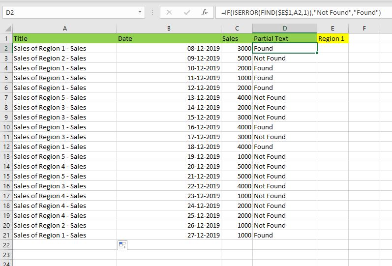
- Проверяем условие для полного совпадения текста.
- ЕСЛИ + СОВПАД
- Использование функции ЕСЛИ с частичным совпадением текста.
- ЕСЛИ + ПОИСК
- ЕСЛИ + НАЙТИ
Будьте особо внимательны в том случае, если для вас важен регистр, в котором записаны ваши текстовые значения. Функция ЕСЛИ не проверяет регистр – это делают функции, которые вы в ней используете. Поясним на примере.
Проверяем условие для полного совпадения текста.
Проверку выполнения
доставки организуем при помощи обычного оператора сравнения «=».
=ЕСЛИ(G2=»выполнено»,ИСТИНА,ЛОЖЬ)
При этом будет не важно,
в каком регистре записаны значения в вашей таблице.

Если же вас интересует
именно точное совпадение текстовых значений с учетом регистра, то можно
рекомендовать вместо оператора «=» использовать функцию СОВПАД(). Она проверяет
идентичность двух текстовых значений с учетом регистра отдельных букв.
Вот как это может
выглядеть на примере.

Обратите внимание, что
если в качестве аргумента мы используем текст, то он обязательно должен быть
заключён в кавычки.
ЕСЛИ + СОВПАД
В случае, если нас интересует полное совпадение текста с заданным условием, включая и регистр его символов, то оператор «=» нам не сможет помочь.
Но мы можем использовать функцию СОВПАД (английский аналог — EXACT).
Функция СОВПАД сравнивает два текста и возвращает ИСТИНА в случае их полного совпадения, и ЛОЖЬ — если есть хотя бы одно отличие, включая регистр букв. Поясним возможность ее использования на примере.
Формула проверки выполнения заказа в столбце Н может выглядеть следующим образом:
=ЕСЛИ(СОВПАД(G2,»Выполнено»),»Да»,»Нет»)

Как видите, варианты «ВЫПОЛНЕНО» и «выполнено» не засчитываются как правильные. Засчитываются только полные совпадения. Будет полезно, если важно точное написание текста — например, в артикулах товаров.
Использование функции ЕСЛИ с частичным совпадением текста.
Выше мы с вами
рассмотрели, как использовать текстовые значения в функции ЕСЛИ. Но часто случается,
что необходимо определить не полное, а частичное совпадение текста с каким-то
эталоном. К примеру, нас интересует город, но при этом совершенно не важно его
название.
Первое, что приходит на
ум – использовать подстановочные знаки «?» и «*» (вопросительный знак и
звездочку). Однако, к сожалению, этот простой способ здесь не проходит.
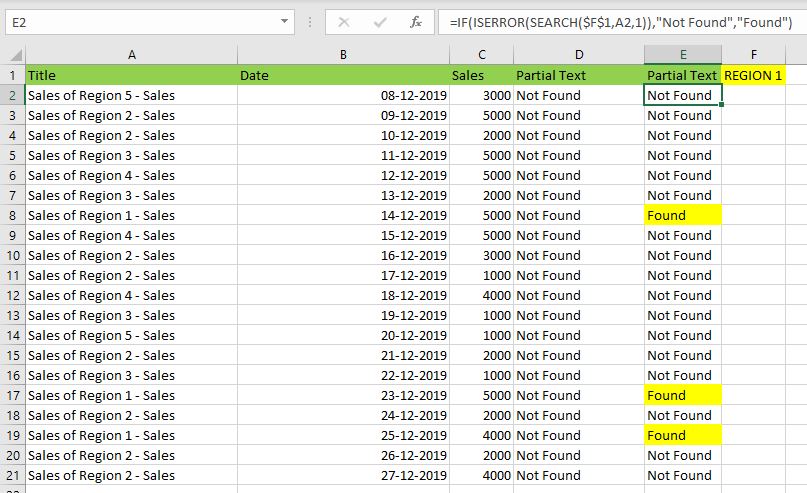
ЕСЛИ + ПОИСК
Нам поможет функция ПОИСК (в английском варианте – SEARCH). Она позволяет определить позицию, начиная с которой искомые символы встречаются в тексте. Синтаксис ее таков:
=ПОИСК(что_ищем, где_ищем, начиная_с_какого_символа_ищем)
Если третий аргумент не
указан, то поиск начинаем с самого начала – с первого символа.
Функция ПОИСК возвращает либо номер позиции, начиная с которой искомые символы встречаются в тексте, либо ошибку.
Но нам для использования в функции ЕСЛИ нужны логические значения.
Здесь нам на помощь приходит еще одна функция EXCEL – ЕЧИСЛО. Если ее аргументом является число, она возвратит логическое значение ИСТИНА. Во всех остальных случаях, в том числе и в случае, если ее аргумент возвращает ошибку, ЕЧИСЛО возвратит ЛОЖЬ.
В итоге наше выражение в
ячейке G2
будет выглядеть следующим образом:
=ЕСЛИ(ЕЧИСЛО(ПОИСК(«город»,B2)),»Город»,»»)
Еще одно важное уточнение. Функция ПОИСК не различает регистр символов.

ЕСЛИ + НАЙТИ
В том случае, если для нас важны строчные и прописные буквы, то придется использовать вместо нее функцию НАЙТИ (в английском варианте – FIND).
Синтаксис ее совершенно аналогичен функции ПОИСК: что ищем, где ищем, начиная с какой позиции.
Изменим нашу формулу в
ячейке G2
=ЕСЛИ(ЕЧИСЛО(НАЙТИ(«город»,B2)),»Да»,»Нет»)

То есть, если регистр символов для вас важен, просто замените ПОИСК на НАЙТИ.
Итак, мы с вами убедились, что простая на первый взгляд функция ЕСЛИ дает нам на самом деле много возможностей для операций с текстом.
[the_ad_group id=»48″]
Примеры использования функции ЕСЛИ:
 Функция ЕСЛИОШИБКА – примеры формул — В статье описано, как использовать функцию ЕСЛИОШИБКА в Excel для обнаружения ошибок и замены их пустой ячейкой, другим значением или определённым сообщением. Покажем примеры, как использовать функцию ЕСЛИОШИБКА с функциями визуального…
  Сравнение ячеек в Excel — Вы узнаете, как сравнивать значения в ячейках Excel на предмет точного совпадения или без учета регистра. Мы предложим вам несколько формул для сопоставления двух ячеек по их значениям, длине или количеству…
 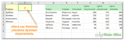 Вычисление номера столбца для извлечения данных в ВПР — Задача: Наиболее простым способом научиться указывать тот столбец, из которого функция ВПР будет извлекать данные. При этом мы не будем изменять саму формулу, поскольку это может привести в случайным ошибкам.…
 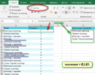 Как проверить правильность ввода данных в Excel? — Подтверждаем правильность ввода галочкой. Задача: При ручном вводе данных в ячейки таблицы проверять правильность ввода в соответствии с имеющимся списком допустимых значений. В случае правильного ввода в отдельном столбце ставить…
 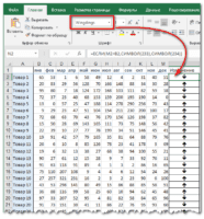 Визуализация данных при помощи функции ЕСЛИ — Функцию ЕСЛИ можно использовать для вставки в таблицу символов, которые наглядно показывают происходящие с данными изменения. К примеру, мы хотим показать в отдельной колонке таблицы, происходит рост или снижение продаж.…
 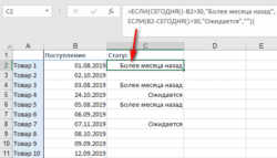 3 примера, как функция ЕСЛИ работает с датами. — На первый взгляд может показаться, что функцию ЕСЛИ для работы с датами можно применять так же, как для числовых и текстовых значений, которые мы только что обсудили. К сожалению, это…
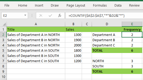
Excel has a number of formulas that help you use your data in useful ways. For example, you can get an output based on whether or not a cell meets certain specifications. Right now, we’ll focus on a function called “if cell contains, then”. Let’s look at an example.
Jump To Specific Section:
- Explanation: If Cell Contains
- If cell contains any value, then return a value
- If cell contains text/number, then return a value
- If cell contains specific text, then return a value
- If cell contains specific text, then return a value (case-sensitive)
- If cell does not contain specific text, then return a value
- If cell contains one of many text strings, then return a value
- If cell contains several of many text strings, then return a value
Excel Formula: If cell contains
Generic formula
=IF(ISNUMBER(SEARCH("abc",A1)),A1,"")
Summary
To test for cells that contain certain text, you can use a formula that uses the IF function together with the SEARCH and ISNUMBER functions. In the example shown, the formula in C5 is:
=IF(ISNUMBER(SEARCH("abc",B5)),B5,"")
If you want to check whether or not the A1 cell contains the text “Example”, you can run a formula that will output “Yes” or “No” in the B1 cell. There are a number of different ways you can put these formulas to use. At the time of writing, Excel is able to return the following variations:
- If cell contains any value
- If cell contains text
- If cell contains number
- If cell contains specific text
- If cell contains certain text string
- If cell contains one of many text strings
- If cell contains several strings
Using these scenarios, you’re able to check if a cell contains text, value, and more.
Explanation: If Cell Contains
One limitation of the IF function is that it does not support Excel wildcards like «?» and «*». This simply means you can’t use IF by itself to test for text that may appear anywhere in a cell.
One solution is a formula that uses the IF function together with the SEARCH and ISNUMBER functions. For example, if you have a list of email addresses, and want to extract those that contain «ABC», the formula to use is this:
=IF(ISNUMBER(SEARCH("abc",B5)),B5,""). Assuming cells run to B5
If «abc» is found anywhere in a cell B5, IF will return that value. If not, IF will return an empty string («»). This formula’s logical test is this bit:
ISNUMBER(SEARCH("abc",B5))
Read article: Excel efficiency: 11 Excel Formulas To Increase Your Productivity
Using “if cell contains” formulas in Excel
The guides below were written using the latest Microsoft Excel 2019 for Windows 10. Some steps may vary if you’re using a different version or platform. Contact our experts if you need any further assistance.
1. If cell contains any value, then return a value
This scenario allows you to return values based on whether or not a cell contains any value at all. For example, we’ll be checking whether or not the A1 cell is blank or not, and then return a value depending on the result.
- Select the output cell, and use the following formula: =IF(cell<>»», value_to_return, «»).
- For our example, the cell we want to check is A2, and the return value will be No. In this scenario, you’d change the formula to =IF(A2<>»», «No», «»).
- Since the A2 cell isn’t blank, the formula will return “No” in the output cell. If the cell you’re checking is blank, the output cell will also remain blank.
2. If cell contains text/number, then return a value
With the formula below, you can return a specific value if the target cell contains any text or number. The formula will ignore the opposite data types.
Check for text
- To check if a cell contains text, select the output cell, and use the following formula: =IF(ISTEXT(cell), value_to_return, «»).
- For our example, the cell we want to check is A2, and the return value will be Yes. In this scenario, you’d change the formula to =IF(ISTEXT(A2), «Yes», «»).

- Because the A2 cell does contain text and not a number or date, the formula will return “Yes” into the output cell.
Check for a number or date
- To check if a cell contains a number or date, select the output cell, and use the following formula: =IF(ISNUMBER(cell), value_to_return, «»).
- For our example, the cell we want to check is D2, and the return value will be Yes. In this scenario, you’d change the formula to =IF(ISNUMBER(D2), «Yes», «»).

- Because the D2 cell does contain a number and not text, the formula will return “Yes” into the output cell.
3. If cell contains specific text, then return a value
To find a cell that contains specific text, use the formula below.
- Select the output cell, and use the following formula: =IF(cell=»text», value_to_return, «»).
- For our example, the cell we want to check is A2, the text we’re looking for is “example”, and the return value will be Yes. In this scenario, you’d change the formula to =IF(A2=»example», «Yes», «»).

- Because the A2 cell does consist of the text “example”, the formula will return “Yes” into the output cell.
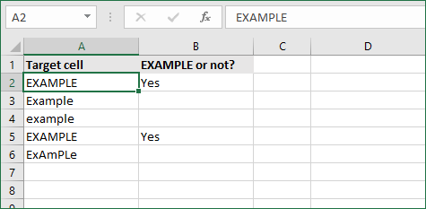
4. If cell contains specific text, then return a value (case-sensitive)
To find a cell that contains specific text, use the formula below. This version is case-sensitive, meaning that only cells with an exact match will return the specified value.
- Select the output cell, and use the following formula: =IF(EXACT(cell,»case_sensitive_text»), «value_to_return», «»).
- For our example, the cell we want to check is A2, the text we’re looking for is “EXAMPLE”, and the return value will be Yes. In this scenario, you’d change the formula to =IF(EXACT(A2,»EXAMPLE»), «Yes», «»).
- Because the A2 cell does consist of the text “EXAMPLE” with the matching case, the formula will return “Yes” into the output cell.
5. If cell does not contain specific text, then return a value
The opposite version of the previous section. If you want to find cells that don’t contain a specific text, use this formula.
- Select the output cell, and use the following formula: =IF(cell=»text», «», «value_to_return»).
- For our example, the cell we want to check is A2, the text we’re looking for is “example”, and the return value will be No. In this scenario, you’d change the formula to =IF(A2=»example», «», «No»).
- Because the A2 cell does consist of the text “example”, the formula will return a blank cell. On the other hand, other cells return “No” into the output cell.
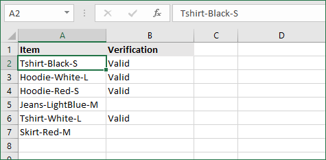
6. If cell contains one of many text strings, then return a value
This formula should be used if you’re looking to identify cells that contain at least one of many words you’re searching for.
- Select the output cell, and use the following formula: =IF(OR(ISNUMBER(SEARCH(«string1», cell)), ISNUMBER(SEARCH(«string2», cell))), value_to_return, «»).
- For our example, the cell we want to check is A2. We’re looking for either “tshirt” or “hoodie”, and the return value will be Valid. In this scenario, you’d change the formula to =IF(OR(ISNUMBER(SEARCH(«tshirt»,A2)),ISNUMBER(SEARCH(«hoodie»,A2))),»Valid «,»»).
- Because the A2 cell does contain one of the text values we searched for, the formula will return “Valid” into the output cell.
To extend the formula to more search terms, simply modify it by adding more strings using ISNUMBER(SEARCH(«string», cell)).
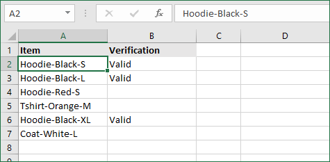
7. If cell contains several of many text strings, then return a value
This formula should be used if you’re looking to identify cells that contain several of the many words you’re searching for. For example, if you’re searching for two terms, the cell needs to contain both of them in order to be validated.
- Select the output cell, and use the following formula: =IF(AND(ISNUMBER(SEARCH(«string1»,cell)), ISNUMBER(SEARCH(«string2″,cell))), value_to_return,»»).
- For our example, the cell we want to check is A2. We’re looking for “hoodie” and “black”, and the return value will be Valid. In this scenario, you’d change the formula to =IF(AND(ISNUMBER(SEARCH(«hoodie»,A2)),ISNUMBER(SEARCH(«black»,A2))),»Valid «,»»).
- Because the A2 cell does contain both of the text values we searched for, the formula will return “Valid” to the output cell.
Final thoughts
We hope this article was useful to you in learning how to use “if cell contains” formulas in Microsoft Excel. Now, you can check if any cells contain values, text, numbers, and more. This allows you to navigate, manipulate and analyze your data efficiently.
We’re glad you’re read the article up to here  Thank you
You may also like
» How to use NPER Function in Excel
» How to Separate First and Last Name in Excel
» How to Calculate Break-Even Analysis in Excel
The IF function runs a logical test and returns one value for a TRUE result, and another value for a FALSE result. The result from IF can be a value, a cell reference, or even another formula. By combining the IF function with other logical functions like AND and OR, you can test more than one condition at a time.
Syntax
The generic syntax for the IF function looks like this:
=IF(logical_test,[value_if_true],[value_if_false])The first argument, logical_test, is typically an expression that returns either TRUE or FALSE. The second argument, value_if_true, is the value to return when logical_test is TRUE. The last argument, value_if_false, is the value to return when logical_test is FALSE. Both value_if_true and value_if_false are optional, but you must provide one or the other. For example, if cell A1 contains 80, then:
=IF(A1>75,TRUE) // returns TRUE
=IF(A1>75,"OK") // returns "OK"
=IF(A1>85,"OK") // returns FALSE
=IF(A1>75,10,0) // returns 10
=IF(A1>85,10,0) // returns 0
=IF(A1>75,"Yes","No") // returns "Yes"
=IF(A1>85,"Yes","No") // returns "No"
Notice that text values like «OK», «Yes», «No», etc. must be enclosed in double quotes («»). However, numeric values should not be enclosed in quotes.
Logical tests
The IF function supports logical operators (>,<,<>,=) when creating logical tests. Most commonly, the logical_test in IF is a complete logical expression that will evaluate to TRUE or FALSE. The table below shows some common examples:
| Goal | Logical test |
|---|---|
| If A1 is greater than 75 | A1>75 |
| If A1 equals 100 | A1=100 |
| If A1 is less than or equal to 100 | A1<=100 |
| If A1 equals «Red» | A1=»red» |
| If A1 is not equal to «Red» | A1<>»red» |
| If A1 is less than B1 | A1<B1 |
| If A1 is empty | A1=»» |
| If A1 is not empty | A1<>»» |
| If A1 is less than current date | A1<TODAY() |
Notice text values must be enclosed in double quotes («»), but numbers do not. The IF function does not support wildcards, but you can combine IF with COUNTIF to get basic wildcard functionality. To test for substrings in a cell, you can use the IF function with the SEARCH function.
Pass or Fail example
In the worksheet shown above, we want to assign either «Pass» or «Fail» based on a test score. A passing score is 70 or higher. The formula in D6, copied down, is:
=IF(C5>=70,"Pass","Fail")
Translation: If the value in C5 is greater than or equal to 70, return «Pass». Otherwise, return «Fail».
Note that the logical flow of this formula can be reversed. This formula returns the same result:
=IF(C5<70,"Fail","Pass")
Translation: If the value in C5 is less than 70, return «Fail». Otherwise, return «Pass».
Both formulas above, when copied down, will return correct results.
Note: If you are new to the idea of formula criteria, this article explains many examples.
Assign points based on color
In the worksheet below, we want to assign points based on the color in column B. If the color is «red», the result should be 100. If the color is «blue», the result should be 125. This requires that we use a formula based on two IF functions, one nested inside the other. The formula in C5, copied down, is:
=IF(B5="red",100,IF(B5="blue",125))
Translation: IF the value in B5 is «red», return 100. Else, if the value in B5 is «blue», return 125.

There are three things to notice in this example:
- The formula will return FALSE if the value in B5 is anything except «red» or «blue»
- The text values «red» and «blue» must be enclosed in double quotes («»)
- The IF function is not case-sensitive and will match «red», «Red», «RED», or «rEd».
This is a simple example of a nested IFs formula. See below for a more complex example.
Return another formula
The IF function can return another formula as a result. For example, the formula below will return A1*5% when A1 is less than 100, and A1*7% when A1 is greater than or equal to 100:
=IF(A1<100,A1*5%,A1*7%)
Nested IF statements
The IF function can be «nested». A «nested IF» refers to a formula where at least one IF function is nested inside another in order to test for more conditions and return more possible results. Each IF statement needs to be carefully «nested» inside another so that the logic is correct. For example, the following formula can be used to assign a grade rather than a pass / fail result:
=IF(C6<70,"F",IF(C6<75,"D",IF(C6<85,"C",IF(C6<95,"B","A"))))
Up to 64 IF functions can be nested. However, in general, you should consider other functions, like VLOOKUP or XLOOKUP for more complex scenarios, because they can handle more conditions in a more streamlined fashion. For a more details see this article on nested IFs.
Note: the newer IFS function is designed to handle multiple conditions without nesting. However, a lookup function like VLOOKUP or XLOOKUP is usually a better approach unless the logic for each condition is custom.
IF with AND, OR, NOT
The IF function can be combined with the AND function and the OR function. For example, to return «OK» when A1 is between 7 and 10, you can use a formula like this:
=IF(AND(A1>7,A1<10),"OK","")
Translation: if A1 is greater than 7 and less than 10, return «OK». Otherwise, return nothing («»).
To return B1+10 when A1 is «red» or «blue» you can use the OR function like this:
=IF(OR(A1="red",A1="blue"),B1+10,B1)
Translation: if A1 is red or blue, return B1+10, otherwise return B1.
=IF(NOT(A1="red"),B1+10,B1)
Translation: if A1 is NOT red, return B1+10, otherwise return B1.
IF cell contains specific text
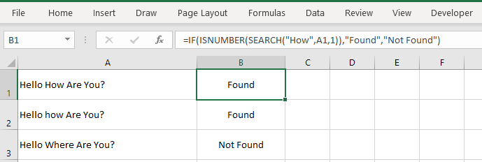
Because the IF function does not support wildcards, it is not obvious how to configure IF to check for a specific substring in a cell. A common approach is to combine the ISNUMBER function and the SEARCH function to create a logical test like this:
=ISNUMBER(SEARCH(substring,A1)) // returns TRUE or FALSEFor example, to check for the substring «xyz» in cell A1, you can use a formula like this:
=IF(ISNUMBER(SEARCH("xyz",A1)),"Yes","No")Read a detailed explanation here.
More information
- Read more about nested IFs
- Learn how to use VLOOKUP instead of nested IFs (video)
- 50 Examples of formula criteria
Notes
- The IF function is not case-sensitive.
- To count values conditionally, use the COUNTIF or the COUNTIFS functions.
- To sum values conditionally, use the SUMIF or the SUMIFS functions.
- If any of the arguments to IF are supplied as arrays, the IF function will evaluate every element of the array.
![]()
Excel If Cell Contains Text

Excel If Cell Contains Text Then Formula helps you to return the output when a cell have any text or a specific text. You can check if a cell contains a some string or text and produce something in other cell. For Example you can check if a cell A1 contains text ‘example text’ and print Yes or No in Cell B1. Following are the example Formulas to check if Cell contains text then return some thing in a Cell.
If Cell Contains Text
Here are the Excel formulas to check if Cell contains specific text then return something. This will return if there is any string or any text in given Cell. We can use this simple approach to check if a cell contains text, specific text, string, any text using Excel If formula. We can use equals to operator(=) to compare the strings .
If Cell Contains Text Then TRUE
Following is the Excel formula to return True if a Cell contains Specif Text. You can check a cell if there is given string in the Cell and return True or False.
The formula will return true if it found the match, returns False of no match found.
If Cell Contains Partial Text
We can return Text If Cell Contains Partial Text. We use formula or VBA to Check Partial Text in a Cell.
Find for Case Sensitive Match:
We can check if a Cell Contains Partial Text then return something using Excel Formula. Following is a simple example to find the partial text in a given Cell. We can use if your want to make the criteria case sensitive.
- Here, Find Function returns the finding position of the given string
- Use Find function is Case Sensitive
- IsError Function check if Find Function returns Error, that means, string not found
Search for Not Case Sensitive Match:
We can use Search function to check if Cell Contains Partial Text. Search function useful if you want to make the checking criteria Not Case Sensitive.
If Range of Cells Contains Text
We can check for the strings in a range of cells. Here is the formula to find If Range of Cells Contains Text. We can use Count If Formula to check the excel if range of cells contains specific text and return Text.
- CountIf function counts the number of cells with given criteria
- We can use If function to return the required Text
- Formula displays the Text ‘Range Contains Text” if match found
- Returns “Text Not Found in the Given Range” if match not found in the specified range
If Cells Contains Text From List
Below formulas returns text If Cells Contains Text from given List. You can use based on your requirement.
VlookUp to Check If Cell Contains Text from a List:
We can use VlookUp function to match the text in the Given list of Cells. And return the corresponding values.
- Check if a List Contains Text:
=IF(ISERR(VLOOKUP(F1,A1:B21,2,FALSE)),”False:Not Contains”,”True: Text Found”) - Check if a List Contains Text and Return Corresponding Value:
=VLOOKUP(F1,A1:B21,2,FALSE) - Check if a List Contains Partial Text and Return its Value:
=VLOOKUP(“*”&F1&”*”,A1:B21,2,FALSE)
If Cell Contains Text Then Return a Value
We can return some value if cell contains some string. Here is the the the Excel formula to return a value if a Cell contains Text. You can check a cell if there is given string in the Cell and return some string or value in another column.
The formula will return true if it found the match, returns False of no match found. can
Excel if cell contains word then assign value
You can replace any word in the following formula to check if cell contains word then assign value.
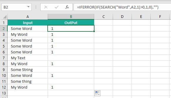
Search function will check for a given word in the required cell and return it’s position. We can use If function to check if the value is greater than 0 and assign a given value (example: 1) in the cell. search function returns #Value if there is no match found in the cell, we can handle this using IFERROR function.
Count If Cell Contains Text
We can check If Cell Contains Text Then COUNT. Here is the Excel formula to Count if a Cell contains Text. You can count the number of cells containing specific text.
The formula will Sum the values in Column B if the cells of Column A contains the given text.
Count If Cell Contains Partial Text
We can count the cells based on partial match criteria. The following Excel formula Counts if a Cell contains Partial Text.
- We can use the CountIf Function to Count the Cells if they contains given String
- Wild-card operators helps to make the CountIf to check for the Partial String
- Put Your Text between two asterisk symbols (*YourText*) to make the criteria to find any where in the given Cell
- Add Asterisk symbol at end of your text (YourText*) to make the criteria to find your text beginning of given Cell
- Place Asterisk symbol at beginning of your text (*YourText) to make the criteria to find your text end of given Cell
If Cell contains text from list then return value
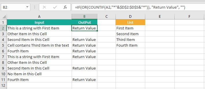
Here is the Excel Formula to check if cell contains text from list then return value. We can use COUNTIF and OR function to check the array of values in a Cell and return the given Value. Here is the formula to check the list in range D2:D5 and check in Cell A2 and return value in B2.
If Cell Contains Text Then SUM
Following is the Excel formula to Sum if a Cell contains Text. You can total the cell values if there is given string in the Cell. Here is the example to sum the column B values based on the values in another Column.
The formula will Sum the values in Column B if the cells of Column A contains the given text.

Sum If Cell Contains Partial Text
Use SumIfs function to Sum the cells based on partial match criteria. The following Excel formula Sums the Values if a Cell contains Partial Text.
- SUMIFS Function will Sum the Given Sum Range
- We can specify the Criteria Range, and wild-card expression to check for the Partial text
- Put Your Text between two asterisk symbols (*YourText*) to Sum the Cells if the criteria to find any where in the given Cell
- Add Asterisk symbol at end of your text (YourText*) to Sum the Cells if the criteria to find your text beginning of given Cell
- Place Asterisk symbol at beginning of your text (*YourText) to Sum the Cells if criteria to find your text end of given Cell
VBA to check if Cell Contains Text
Here is the VBA function to find If Cells Contains Text using Excel VBA Macros.
If Cell Contains Partial Text VBA
We can use VBA to check if Cell Contains Text and Return Value. Here is the simple VBA code match the partial text. Excel VBA if Cell contains partial text macros helps you to use in your procedures and functions.
MsgBox CheckIfCellContainsPartialText(Cells(2, 1), “Region 1”)
End Sub
Function CheckIfCellContainsPartialText(ByVal cell As Range, ByVal strText As String) As Boolean
If InStr(1, cell.Value, strText) > 0 Then CheckIfCellContainsPartialText = True
End Function
- CheckIfCellContainsPartialText VBA Function returns true if Cell Contains Partial Text
- inStr Function will return the Match Position in the given string
If Cell Contains Text Then VBA MsgBox
Here is the simple VBA code to display message box if cell contains text. We can use inStr Function to search for the given string. And show the required message to the user.
If InStr(1, Cells(2, 1), “Region 3”) > 0 Then blnMatch = True
If blnMatch = True Then MsgBox “Cell Contains Text”
End Sub
- inStr Function will return the Match Position in the given string
- blnMatch is the Boolean variable becomes True when match string
- You can display the message to the user if a Range Contains Text
Which function returns true if cell a1 contains text?
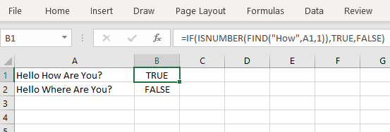
You can use the Excel If function and Find function to return TRUE if Cell A1 Contains Text. Here is the formula to return True.
Which function returns true if cell a1 contains text value?
You can use the Excel If function with Find function to return TRUE if a Cell A1 Contains Text Value. Below is the formula to return True based on the text value.
Share This Story, Choose Your Platform!
7 Comments
-
Meghana
December 27, 2019 at 1:42 pm — ReplyHi Sir,Thank you for the great explanation, covers everything and helps use create formulas if cell contains text values.
Many thanks! Meghana!!
-
Max
December 27, 2019 at 4:44 pm — ReplyPerfect! Very Simple and Clear explanation. Thanks!!
-
Mike Song
August 29, 2022 at 2:45 pm — ReplyI tried this exact formula and it did not work.
-
Theresa A Harding
October 18, 2022 at 9:51 pm — Reply -
Marko
November 3, 2022 at 9:21 pm — ReplyHi
Is possible to sum all WA11?
(A1) WA11 4
(A2) AdBlue 1, WA11 223
(A3) AdBlue 3, WA11 32, shift 4
… and everything is in one column.
Thanks you very much for your help.
Sincerely Marko
-
Mike
December 9, 2022 at 9:59 pm — ReplyThank you for the help. The formula =OR(COUNTIF(M40,”*”&Vendors&”*”)) will give “TRUE” when some part of M40 contains a vendor from “Vendors” list. But how do I get Excel to tell which vendor it found in the M40 cell?
-
PNRao
December 18, 2022 at 6:05 am — ReplyPlease describe your question more elaborately.
Thanks!
-
© Copyright 2012 – 2020 | Excelx.com | All Rights Reserved
Page load link
EXPLANATION
This tutorial shows how to test if a cell contains text and return a specified value if the test is True or False by using Excel formulas or VBA.
This tutorial provides three Excel methods that can be applied to test if a cell contains text.
The first method uses a combination of an Excel IF and ISTEXT functions. The ISTEXT function test if the selected cell contains text. If it does then the function will return a TRUE value. The IF function is then used to return a specified value if the ISTEXT function returns a value of TRUE, which in this example is «Contains Text». Alternatively, if the ISTEXT function returns a value of FALSE, then the cell does not contain text and the IF function will return the associated value, which in this example is «No Text».
The second method uses a combination of an Excel IF and ISNUMBER functions. The ISNUMBER function test if the selected cell is a numeric value. If the cell is a numeric value, meaning that there are no text values, then the function will return a TRUE value, alternatively if the cell contains a text value, the function will return a FALSE value. The IF function is then used to return a specified value if the ISNUMBER function returns a value of FALSE, which in this example is «Contains Text». Alternatively, if the ISNUMBER function returns a value of TRUE, then the cell does not contain text and the IF function will return the associated value, which in this example is «No Text».
The third method uses a combination of an Excel IF and COUNTIF functions. The COUNTIF function uses the «*» to identify if the cell contains text. If the cell contains text the COUNTIF function will return a value of 1, alternatively it will return a value of 0. The IF function is then used to return a specified value if the COUNTIF function returns a value greater than 0, which in this example is «Contains Text». Alternatively, if the COUNTIF function returns a value of 0, then the cell does not contain text and the IF function will return the associated value, which in this example is «No Text».
This tutorial provides six VBA methods that can be applied to test if a cell contains text and return a specific value. Methods 1, 3 and 5 are applied against a single cell, whilst methods 2, 4 and 6 use a For Loop to loop through all of the relevant cells, as per the example in the image, to test each of the cells in a range and return specific values. The main difference between the examples is how the code determines is the cell contains text.
FORMULA (using ISTEXT function)
=IF(ISTEXT(value)=TRUE, value_if_true, value_if_false)
FORMULA (using ISNUMBER function)
=IF(ISNUMBER(value)=FALSE, value_if_true, value_if_false)
FORMULA (using COUNTIF function)
=IF(COUNTIF(value, «*»)>0, value_if_true, value_if_false)
ARGUMENTS
value: The value or cell that is to be tested.
value_if_true: Value to be returned if the value or cell contains text.
value_if_false: Value to be returned if the value or cell does not contains text.