
Normally, If you want to write an IF formula for text values in combining with the below two logical operators in excel, such as: “equal to” or “not equal to”.
Table of Contents
- Excel IF function check if a cell contains text(case-insensitive)
- Excel IF function check if a cell contains text (case-sensitive)
- Excel IF function check if part of cell matches specific text
- Excel IF function with Wildcards text value
- Related Formulas
- Related Functions
Excel IF function check if a cell contains text(case-insensitive)
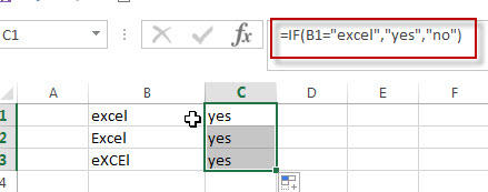
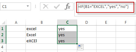
By default, IF function is case-insensitive in excel. It means that the logical text for text values will do not recognize case in the IF formulas. For example, the following two IF formulas will get the same results when checking the text values in cells.
=IF(B1="excel","yes","no")
=IF(B1="EXCEl","yes","no")
The IF formula will check the values of cell B1 if it is equal to “excel” word, If it is TRUE, then return “yes”, otherwise return “no”. And the logical test in the above IF formula will check the text values in the logical_test argument, whatever the logical_test values are “Excel”, “eXcel”, or “EXCEL”, the IF formula don’t care about that if the text values is in lowercase or uppercase, It will get the same results at last.
Excel IF function check if a cell contains text (case-sensitive)
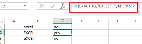
If you want to check text values in cells using IF formula in excel (case-sensitive), then you need to create a case-sensitive logical test and then you can use IF function in combination with EXACT function to compare two text values. So if those two text values are exactly the same, then return TRUE. Otherwise return FALSE.
So we can write down the following IF formula combining with EXACT function:
=IF(EXACT(B1,"excel"),"yes","no")
Excel IF function check if part of cell matches specific text
If you want to check if part of text values in cell matches the specific text rather than exact match, to achieve this logic text, you can use IF function in combination with ISNUMBER and SEARCH Function in excel.
Both ISNUMBER and SEARCH functions are case-insensitive in excel.
=IF(ISNUMBER(SEARCH("x",B1)),"good","bad")
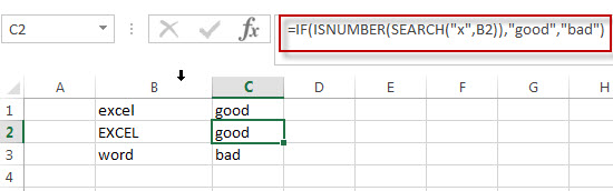
For above the IF formula, it will Check to see if B1 contain the letter x.
Also, we can use FIND function to replace the SEARCH function in the above IF formula. It will return the same results.
Excel IF function with Wildcards text value
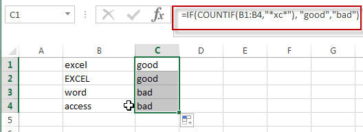
If you wan to use wildcard charcter in an IF formula, for example, if any of the values in column B contains “*xc*”, then return “good”, others return “bad”. You can not directly use the wildcard characters in IF formula, and we can use IF function in combination with COUNTIF function. Let’s see the following IF formula:
=IF(COUNTIF(B1:B4,"*xc*"), "good","bad")
- Excel IF Function With Numbers
If you want to check if a cell values is between two values or checking for the range of numbers or multiple values in cells, at this time, we need to use AND or OR logical function in combination with the logical operator and IF function…
- Excel EXACT function
The Excel SEARCH function returns the number of the starting location of a substring in a text string.The syntax of the EXACT function is as below:= EXACT (text1,text2)… - Excel COUNTIF function
The Excel COUNTIF function will count the number of cells in a range that meet a given criteria.= COUNTIF (range, criteria) … - Excel ISNUMBER function
The Excel ISNUMBER function returns TRUE if the value in a cell is a numeric value, otherwise it will return FALSE. - Excel IF function
The Excel IF function perform a logical test to return one value if the condition is TRUE and return another value if the condition is FALSE…. - Excel SEARCH function
The Excel SEARCH function returns the number of the starting location of a substring in a text string.…
Содержание
- IF function
- Simple IF examples
- Common problems
- Need more help?
- How To Use “If Cell Contains” Formulas in Excel
- Excel Formula: If cell contains
- Explanation: If Cell Contains
- Using “if cell contains” formulas in Excel
- 1. If cell contains any value, then return a value
- 2. If cell contains text/number, then return a value
- Check for text
- Check for a number or date
- 3. If cell contains specific text, then return a value
- 4. If cell contains specific text, then return a value (case-sensitive)
- 5. If cell does not contain specific text, then return a value
- 6. If cell contains one of many text strings, then return a value
- 7. If cell contains several of many text strings, then return a value
- Final thoughts
- Before you go
- Excel IF function with text values
- Excel IF function check if a cell contains text(case-insensitive)
- Excel IF function check if a cell contains text (case-sensitive)
- Excel IF function check if part of cell matches specific text
- Excel IF function with Wildcards text value
IF function
The IF function is one of the most popular functions in Excel, and it allows you to make logical comparisons between a value and what you expect.
So an IF statement can have two results. The first result is if your comparison is True, the second if your comparison is False.
For example, =IF(C2=”Yes”,1,2) says IF(C2 = Yes, then return a 1, otherwise return a 2).

Use the IF function, one of the logical functions, to return one value if a condition is true and another value if it’s false.
IF(logical_test, value_if_true, [value_if_false])
The condition you want to test.
The value that you want returned if the result of logical_test is TRUE.
The value that you want returned if the result of logical_test is FALSE.
Simple IF examples

In the above example, cell D2 says: IF(C2 = Yes, then return a 1, otherwise return a 2)

In this example, the formula in cell D2 says: IF(C2 = 1, then return Yes, otherwise return No)As you see, the IF function can be used to evaluate both text and values. It can also be used to evaluate errors. You are not limited to only checking if one thing is equal to another and returning a single result, you can also use mathematical operators and perform additional calculations depending on your criteria. You can also nest multiple IF functions together in order to perform multiple comparisons.
 B2,”Over Budget”,”Within Budget”)» loading=»lazy»>
=IF(C2>B2,”Over Budget”,”Within Budget”)
In the above example, the IF function in D2 is saying IF(C2 Is Greater Than B2, then return “Over Budget”, otherwise return “Within Budget”)
 B2,C2-B2,»»)» loading=»lazy»>
In the above illustration, instead of returning a text result, we are going to return a mathematical calculation. So the formula in E2 is saying IF(Actual is Greater than Budgeted, then Subtract the Budgeted amount from the Actual amount, otherwise return nothing).

In this example, the formula in F7 is saying IF(E7 = “Yes”, then calculate the Total Amount in F5 * 8.25%, otherwise no Sales Tax is due so return 0)
Note: If you are going to use text in formulas, you need to wrap the text in quotes (e.g. “Text”). The only exception to that is using TRUE or FALSE, which Excel automatically understands.
Common problems
What went wrong
There was no argument for either value_if_true or value_if_False arguments. To see the right value returned, add argument text to the two arguments, or add TRUE or FALSE to the argument.
This usually means that the formula is misspelled.
Need more help?
You can always ask an expert in the Excel Tech Community or get support in the Answers community.
Источник
How To Use “If Cell Contains” Formulas in Excel
Excel has a number of formulas that help you use your data in useful ways. For example, you can get an output based on whether or not a cell meets certain specifications. Right now, we’ll focus on a function called “if cell contains, then”. Let’s look at an example.

Excel Formula: If cell contains
To test for cells that contain certain text, you can use a formula that uses the IF function together with the SEARCH and ISNUMBER functions. In the example shown, the formula in C5 is:
If you want to check whether or not the A1 cell contains the text “Example”, you can run a formula that will output “Yes” or “No” in the B1 cell. There are a number of different ways you can put these formulas to use. At the time of writing, Excel is able to return the following variations:
- If cell contains any value
- If cell contains text
- If cell contains number
- If cell contains specific text
- If cell contains certain text string
- If cell contains one of many text strings
- If cell contains several strings
Using these scenarios, you’re able to check if a cell contains text, value, and more.
Explanation: If Cell Contains
One limitation of the IF function is that it does not support Excel wildcards like «?» and «*». This simply means you can’t use IF by itself to test for text that may appear anywhere in a cell.
One solution is a formula that uses the IF function together with the SEARCH and ISNUMBER functions. For example, if you have a list of email addresses, and want to extract those that contain «ABC», the formula to use is this:
If «abc» is found anywhere in a cell B5, IF will return that value. If not, IF will return an empty string («»). This formula’s logical test is this bit:
Using “if cell contains” formulas in Excel
The guides below were written using the latest Microsoft Excel 2019 for Windows 10 . Some steps may vary if you’re using a different version or platform. Contact our experts if you need any further assistance.
1. If cell contains any value, then return a value
This scenario allows you to return values based on whether or not a cell contains any value at all. For example, we’ll be checking whether or not the A1 cell is blank or not, and then return a value depending on the result.
- Select the output cell, and use the following formula: =IF(cell<>«», value_to_return, «») .
- For our example, the cell we want to check is A2 , and the return value will be No . In this scenario, you’d change the formula to =IF(A2<>«», «No», «») .
2. If cell contains text/number, then return a value
With the formula below, you can return a specific value if the target cell contains any text or number. The formula will ignore the opposite data types.
Check for text
- To check if a cell contains text, select the output cell, and use the following formula: =IF(ISTEXT(cell), value_to_return, «») .
- For our example, the cell we want to check is A2 , and the return value will be Yes . In this scenario, you’d change the formula to =IF(ISTEXT(A2), «Yes», «») .

- Because the A2 cell does contain text and not a number or date, the formula will return “ Yes ” into the output cell.
Check for a number or date
- To check if a cell contains a number or date, select the output cell, and use the following formula: =IF(ISNUMBER(cell), value_to_return, «») .
- For our example, the cell we want to check is D2 , and the return value will be Yes . In this scenario, you’d change the formula to =IF(ISNUMBER(D2), «Yes», «») .
- Because the D2 cell does contain a number and not text, the formula will return “ Yes ” into the output cell.
3. If cell contains specific text, then return a value
To find a cell that contains specific text, use the formula below.
- Select the output cell, and use the following formula: =IF(cell=»text», value_to_return, «») .
- For our example, the cell we want to check is A2 , the text we’re looking for is “ example ”, and the return value will be Yes . In this scenario, you’d change the formula to =IF(A2=»example», «Yes», «») .
- Because the A2 cell does consist of the text “ example ”, the formula will return “ Yes ” into the output cell.
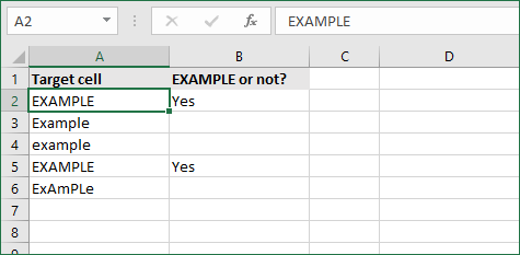
4. If cell contains specific text, then return a value (case-sensitive)
To find a cell that contains specific text, use the formula below. This version is case-sensitive, meaning that only cells with an exact match will return the specified value.
- Select the output cell, and use the following formula: =IF(EXACT(cell,»case_sensitive_text»), «value_to_return», «») .
- For our example, the cell we want to check is A2 , the text we’re looking for is “ EXAMPLE ”, and the return value will be Yes . In this scenario, you’d change the formula to =IF(EXACT(A2,»EXAMPLE»), «Yes», «») .
- Because the A2 cell does consist of the text “ EXAMPLE ” with the matching case, the formula will return “ Yes ” into the output cell.
5. If cell does not contain specific text, then return a value
The opposite version of the previous section. If you want to find cells that don’t contain a specific text, use this formula.
- Select the output cell, and use the following formula: =IF(cell=»text», «», «value_to_return») .
- For our example, the cell we want to check is A2 , the text we’re looking for is “ example ”, and the return value will be No . In this scenario, you’d change the formula to =IF(A2=»example», «», «No») .
- Because the A2 cell does consist of the text “ example ”, the formula will return a blank cell. On the other hand, other cells return “ No ” into the output cell.
6. If cell contains one of many text strings, then return a value
This formula should be used if you’re looking to identify cells that contain at least one of many words you’re searching for.
- Select the output cell, and use the following formula: =IF(OR(ISNUMBER(SEARCH(«string1», cell)), ISNUMBER(SEARCH(«string2», cell))), value_to_return, «») .
- For our example, the cell we want to check is A2 . We’re looking for either “ tshirt ” or “ hoodie ”, and the return value will be Valid . In this scenario, you’d change the formula to =IF(OR(ISNUMBER(SEARCH(«tshirt»,A2)),ISNUMBER(SEARCH(«hoodie»,A2))),»Valid «,»») .
- Because the A2 cell does contain one of the text values we searched for, the formula will return “ Valid ” into the output cell.
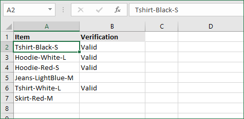
To extend the formula to more search terms, simply modify it by adding more strings using ISNUMBER(SEARCH(«string», cell)) .
7. If cell contains several of many text strings, then return a value
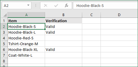
This formula should be used if you’re looking to identify cells that contain several of the many words you’re searching for. For example, if you’re searching for two terms, the cell needs to contain both of them in order to be validated.
- Select the output cell, and use the following formula: =IF(AND(ISNUMBER(SEARCH(«string1»,cell)), ISNUMBER(SEARCH(«string2″,cell))), value_to_return,»») .
- For our example, the cell we want to check is A2 . We’re looking for “ hoodie ” and “ black ”, and the return value will be Valid . In this scenario, you’d change the formula to =IF(AND(ISNUMBER(SEARCH(«hoodie»,A2)),ISNUMBER(SEARCH(«black»,A2))),»Valid «,»») .
- Because the A2 cell does contain both of the text values we searched for, the formula will return “ Valid ” to the output cell.
Final thoughts
We hope this article was useful to you in learning how to use “if cell contains” formulas in Microsoft Excel. Now, you can check if any cells contain values, text, numbers, and more. This allows you to navigate, manipulate and analyze your data efficiently.
We’re glad you’re read the article up to here 🙂 Thank you 🙂
Please share it on your socials. Someone else will benefit.
Before you go
If you need any further help with Excel, don’t hesitate to reach out to our customer service team, which is available 24/7 to assist you. Return to us for more informative articles all related to productivity and modern-day technology!
Would you like to receive promotions, deals, and discounts to get our products for the best price? Don’t forget to subscribe to our newsletter by entering your email address below! Receive the latest technology news in your inbox and be the first to read our tips to become more productive.
Источник
Excel IF function with text values
Normally, If you want to write an IF formula for text values in combining with the below two logical operators in excel, such as: “equal to” or “not equal to”.
Excel IF function check if a cell contains text(case-insensitive)
By default, IF function is case-insensitive in excel. It means that the logical text for text values will do not recognize case in the IF formulas. For example, the following two IF formulas will get the same results when checking the text values in cells.
The IF formula will check the values of cell B1 if it is equal to “excel” word, If it is TRUE, then return “yes”, otherwise return “no”. And the logical test in the above IF formula will check the text values in the logical_test argument, whatever the logical_test values are “Excel”, “eXcel”, or “EXCEL”, the IF formula don’t care about that if the text values is in lowercase or uppercase, It will get the same results at last.
Excel IF function check if a cell contains text (case-sensitive)
If you want to check text values in cells using IF formula in excel (case-sensitive), then you need to create a case-sensitive logical test and then you can use IF function in combination with EXACT function to compare two text values. So if those two text values are exactly the same, then return TRUE. Otherwise return FALSE.
So we can write down the following IF formula combining with EXACT function:
Excel IF function check if part of cell matches specific text
If you want to check if part of text values in cell matches the specific text rather than exact match, to achieve this logic text, you can use IF function in combination with ISNUMBER and SEARCH Function in excel.
Both ISNUMBER and SEARCH functions are case-insensitive in excel.
For above the IF formula, it will Check to see if B1 contain the letter x.
Also, we can use FIND function to replace the SEARCH function in the above IF formula. It will return the same results.
Excel IF function with Wildcards text value
If you wan to use wildcard charcter in an IF formula, for example, if any of the values in column B contains “*xc*”, then return “good”, others return “bad”. You can not directly use the wildcard characters in IF formula, and we can use IF function in combination with COUNTIF function. Let’s see the following IF formula:
Источник
Excel has a number of formulas that help you use your data in useful ways. For example, you can get an output based on whether or not a cell meets certain specifications. Right now, we’ll focus on a function called “if cell contains, then”. Let’s look at an example.
Jump To Specific Section:
- Explanation: If Cell Contains
- If cell contains any value, then return a value
- If cell contains text/number, then return a value
- If cell contains specific text, then return a value
- If cell contains specific text, then return a value (case-sensitive)
- If cell does not contain specific text, then return a value
- If cell contains one of many text strings, then return a value
- If cell contains several of many text strings, then return a value
Excel Formula: If cell contains
Generic formula
=IF(ISNUMBER(SEARCH("abc",A1)),A1,"")
Summary
To test for cells that contain certain text, you can use a formula that uses the IF function together with the SEARCH and ISNUMBER functions. In the example shown, the formula in C5 is:
=IF(ISNUMBER(SEARCH("abc",B5)),B5,"")
If you want to check whether or not the A1 cell contains the text “Example”, you can run a formula that will output “Yes” or “No” in the B1 cell. There are a number of different ways you can put these formulas to use. At the time of writing, Excel is able to return the following variations:
- If cell contains any value
- If cell contains text
- If cell contains number
- If cell contains specific text
- If cell contains certain text string
- If cell contains one of many text strings
- If cell contains several strings
Using these scenarios, you’re able to check if a cell contains text, value, and more.
Explanation: If Cell Contains
One limitation of the IF function is that it does not support Excel wildcards like «?» and «*». This simply means you can’t use IF by itself to test for text that may appear anywhere in a cell.
One solution is a formula that uses the IF function together with the SEARCH and ISNUMBER functions. For example, if you have a list of email addresses, and want to extract those that contain «ABC», the formula to use is this:
=IF(ISNUMBER(SEARCH("abc",B5)),B5,""). Assuming cells run to B5
If «abc» is found anywhere in a cell B5, IF will return that value. If not, IF will return an empty string («»). This formula’s logical test is this bit:
ISNUMBER(SEARCH("abc",B5))
Read article: Excel efficiency: 11 Excel Formulas To Increase Your Productivity
Using “if cell contains” formulas in Excel
The guides below were written using the latest Microsoft Excel 2019 for Windows 10. Some steps may vary if you’re using a different version or platform. Contact our experts if you need any further assistance.
1. If cell contains any value, then return a value
This scenario allows you to return values based on whether or not a cell contains any value at all. For example, we’ll be checking whether or not the A1 cell is blank or not, and then return a value depending on the result.
- Select the output cell, and use the following formula: =IF(cell<>»», value_to_return, «»).
- For our example, the cell we want to check is A2, and the return value will be No. In this scenario, you’d change the formula to =IF(A2<>»», «No», «»).
- Since the A2 cell isn’t blank, the formula will return “No” in the output cell. If the cell you’re checking is blank, the output cell will also remain blank.
2. If cell contains text/number, then return a value
With the formula below, you can return a specific value if the target cell contains any text or number. The formula will ignore the opposite data types.
Check for text
- To check if a cell contains text, select the output cell, and use the following formula: =IF(ISTEXT(cell), value_to_return, «»).
- For our example, the cell we want to check is A2, and the return value will be Yes. In this scenario, you’d change the formula to =IF(ISTEXT(A2), «Yes», «»).

- Because the A2 cell does contain text and not a number or date, the formula will return “Yes” into the output cell.
Check for a number or date
- To check if a cell contains a number or date, select the output cell, and use the following formula: =IF(ISNUMBER(cell), value_to_return, «»).
- For our example, the cell we want to check is D2, and the return value will be Yes. In this scenario, you’d change the formula to =IF(ISNUMBER(D2), «Yes», «»).

- Because the D2 cell does contain a number and not text, the formula will return “Yes” into the output cell.
3. If cell contains specific text, then return a value
To find a cell that contains specific text, use the formula below.
- Select the output cell, and use the following formula: =IF(cell=»text», value_to_return, «»).
- For our example, the cell we want to check is A2, the text we’re looking for is “example”, and the return value will be Yes. In this scenario, you’d change the formula to =IF(A2=»example», «Yes», «»).

- Because the A2 cell does consist of the text “example”, the formula will return “Yes” into the output cell.
4. If cell contains specific text, then return a value (case-sensitive)
To find a cell that contains specific text, use the formula below. This version is case-sensitive, meaning that only cells with an exact match will return the specified value.
- Select the output cell, and use the following formula: =IF(EXACT(cell,»case_sensitive_text»), «value_to_return», «»).
- For our example, the cell we want to check is A2, the text we’re looking for is “EXAMPLE”, and the return value will be Yes. In this scenario, you’d change the formula to =IF(EXACT(A2,»EXAMPLE»), «Yes», «»).
- Because the A2 cell does consist of the text “EXAMPLE” with the matching case, the formula will return “Yes” into the output cell.
5. If cell does not contain specific text, then return a value
The opposite version of the previous section. If you want to find cells that don’t contain a specific text, use this formula.
- Select the output cell, and use the following formula: =IF(cell=»text», «», «value_to_return»).
- For our example, the cell we want to check is A2, the text we’re looking for is “example”, and the return value will be No. In this scenario, you’d change the formula to =IF(A2=»example», «», «No»).
- Because the A2 cell does consist of the text “example”, the formula will return a blank cell. On the other hand, other cells return “No” into the output cell.
6. If cell contains one of many text strings, then return a value
This formula should be used if you’re looking to identify cells that contain at least one of many words you’re searching for.
- Select the output cell, and use the following formula: =IF(OR(ISNUMBER(SEARCH(«string1», cell)), ISNUMBER(SEARCH(«string2», cell))), value_to_return, «»).
- For our example, the cell we want to check is A2. We’re looking for either “tshirt” or “hoodie”, and the return value will be Valid. In this scenario, you’d change the formula to =IF(OR(ISNUMBER(SEARCH(«tshirt»,A2)),ISNUMBER(SEARCH(«hoodie»,A2))),»Valid «,»»).
- Because the A2 cell does contain one of the text values we searched for, the formula will return “Valid” into the output cell.
To extend the formula to more search terms, simply modify it by adding more strings using ISNUMBER(SEARCH(«string», cell)).
7. If cell contains several of many text strings, then return a value
This formula should be used if you’re looking to identify cells that contain several of the many words you’re searching for. For example, if you’re searching for two terms, the cell needs to contain both of them in order to be validated.
- Select the output cell, and use the following formula: =IF(AND(ISNUMBER(SEARCH(«string1»,cell)), ISNUMBER(SEARCH(«string2″,cell))), value_to_return,»»).
- For our example, the cell we want to check is A2. We’re looking for “hoodie” and “black”, and the return value will be Valid. In this scenario, you’d change the formula to =IF(AND(ISNUMBER(SEARCH(«hoodie»,A2)),ISNUMBER(SEARCH(«black»,A2))),»Valid «,»»).
- Because the A2 cell does contain both of the text values we searched for, the formula will return “Valid” to the output cell.
Final thoughts
We hope this article was useful to you in learning how to use “if cell contains” formulas in Microsoft Excel. Now, you can check if any cells contain values, text, numbers, and more. This allows you to navigate, manipulate and analyze your data efficiently.
We’re glad you’re read the article up to here  Thank you
You may also like
» How to use NPER Function in Excel
» How to Separate First and Last Name in Excel
» How to Calculate Break-Even Analysis in Excel
Range.Value returns a Variant whose subtype depends on the content of the cell.
Given a #N/A, #VALUE, #REF!, or any other cell error value, it returns a Variant/Error that can’t be coerced into anything other than a Variant — trying to compare it to a string or numeric value or expression will throw error 13 «type mismatch».
You can avoid this runtime error by evaluating whether the variant subtype is Error using the IsError function, ideally by capturing the cell’s value into a local Variant variable first, so you don’t have to access the cell twice.
Given an empty cell that has no formula, no value, no content whatsoever, it returns a Variant/Empty; the IsEmpty function can be used to validate this variant subtype.
Given a Date value, it returns a Variant/Date. Given any numeric value, it returns a Variant/Double. Given a TRUE or FALSE value, it returns a Variant/Boolean.
And given a String value, it does return a Variant/String.
Note that the default member of the Range class is a hidden [_Default] property with two optional parameters:
![Property _Default([RowIndex], [ColumnIndex]), default member of Excel.Range](https://i.stack.imgur.com/6VdbV.png)
When no parameters are provided, an explicit call to .Value is equivalent. Explicit member calls should generally be preferred over implicit default member calls, and whether implicit or explicit, the calls should be consistent:
If ws.Cells(3 + j, 3) = "SW" Then ' implicit: .Value
    wssum.Cells(3 + k, 2 + i).Value = busum
Else
    wssum.Cells(3 + k, 14 + i).Value = busum
End If
IF function
The IF function is one of the most popular functions in Excel, and it allows you to make logical comparisons between a value and what you expect.
So an IF statement can have two results. The first result is if your comparison is True, the second if your comparison is False.
For example, =IF(C2=”Yes”,1,2) says IF(C2 = Yes, then return a 1, otherwise return a 2).
Use the IF function, one of the logical functions, to return one value if a condition is true and another value if it’s false.
IF(logical_test, value_if_true, [value_if_false])
For example:
-
=IF(A2>B2,»Over Budget»,»OK»)
-
=IF(A2=B2,B4-A4,»»)
|
Argument name |
Description |
|---|---|
|
logical_test (required) |
The condition you want to test. |
|
value_if_true (required) |
The value that you want returned if the result of logical_test is TRUE. |
|
value_if_false (optional) |
The value that you want returned if the result of logical_test is FALSE. |
Simple IF examples
-
=IF(C2=”Yes”,1,2)
In the above example, cell D2 says: IF(C2 = Yes, then return a 1, otherwise return a 2)
-
=IF(C2=1,”Yes”,”No”)
In this example, the formula in cell D2 says: IF(C2 = 1, then return Yes, otherwise return No)As you see, the IF function can be used to evaluate both text and values. It can also be used to evaluate errors. You are not limited to only checking if one thing is equal to another and returning a single result, you can also use mathematical operators and perform additional calculations depending on your criteria. You can also nest multiple IF functions together in order to perform multiple comparisons.
-
=IF(C2>B2,”Over Budget”,”Within Budget”)
In the above example, the IF function in D2 is saying IF(C2 Is Greater Than B2, then return “Over Budget”, otherwise return “Within Budget”)
-
=IF(C2>B2,C2-B2,0)
In the above illustration, instead of returning a text result, we are going to return a mathematical calculation. So the formula in E2 is saying IF(Actual is Greater than Budgeted, then Subtract the Budgeted amount from the Actual amount, otherwise return nothing).
-
=IF(E7=”Yes”,F5*0.0825,0)
In this example, the formula in F7 is saying IF(E7 = “Yes”, then calculate the Total Amount in F5 * 8.25%, otherwise no Sales Tax is due so return 0)
Note: If you are going to use text in formulas, you need to wrap the text in quotes (e.g. “Text”). The only exception to that is using TRUE or FALSE, which Excel automatically understands.
Common problems
|
Problem |
What went wrong |
|---|---|
|
0 (zero) in cell |
There was no argument for either value_if_true or value_if_False arguments. To see the right value returned, add argument text to the two arguments, or add TRUE or FALSE to the argument. |
|
#NAME? in cell |
This usually means that the formula is misspelled. |
Need more help?
You can always ask an expert in the Excel Tech Community or get support in the Answers community.

See Also
IF function — nested formulas and avoiding pitfalls
IFS function
Using IF with AND, OR and NOT functions
COUNTIF function
How to avoid broken formulas
Overview of formulas in Excel
Need more help?
Want more options?
Explore subscription benefits, browse training courses, learn how to secure your device, and more.
Communities help you ask and answer questions, give feedback, and hear from experts with rich knowledge.
![]()
Excel If Cell Contains Text

Excel If Cell Contains Text Then Formula helps you to return the output when a cell have any text or a specific text. You can check if a cell contains a some string or text and produce something in other cell. For Example you can check if a cell A1 contains text ‘example text’ and print Yes or No in Cell B1. Following are the example Formulas to check if Cell contains text then return some thing in a Cell.
If Cell Contains Text
Here are the Excel formulas to check if Cell contains specific text then return something. This will return if there is any string or any text in given Cell. We can use this simple approach to check if a cell contains text, specific text, string, any text using Excel If formula. We can use equals to operator(=) to compare the strings .
If Cell Contains Text Then TRUE
Following is the Excel formula to return True if a Cell contains Specif Text. You can check a cell if there is given string in the Cell and return True or False.
The formula will return true if it found the match, returns False of no match found.
If Cell Contains Partial Text
We can return Text If Cell Contains Partial Text. We use formula or VBA to Check Partial Text in a Cell.
Find for Case Sensitive Match:
We can check if a Cell Contains Partial Text then return something using Excel Formula. Following is a simple example to find the partial text in a given Cell. We can use if your want to make the criteria case sensitive.
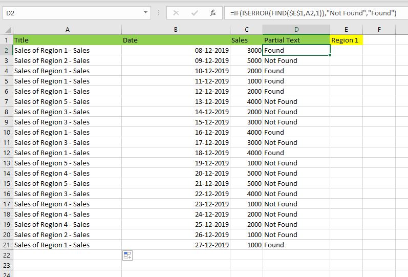
- Here, Find Function returns the finding position of the given string
- Use Find function is Case Sensitive
- IsError Function check if Find Function returns Error, that means, string not found
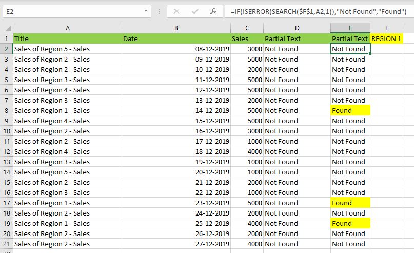
Search for Not Case Sensitive Match:
We can use Search function to check if Cell Contains Partial Text. Search function useful if you want to make the checking criteria Not Case Sensitive.
If Range of Cells Contains Text
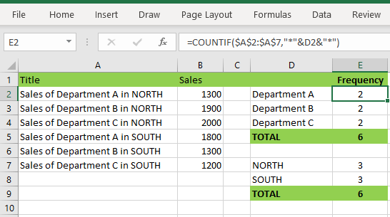
We can check for the strings in a range of cells. Here is the formula to find If Range of Cells Contains Text. We can use Count If Formula to check the excel if range of cells contains specific text and return Text.
- CountIf function counts the number of cells with given criteria
- We can use If function to return the required Text
- Formula displays the Text ‘Range Contains Text” if match found
- Returns “Text Not Found in the Given Range” if match not found in the specified range
If Cells Contains Text From List
Below formulas returns text If Cells Contains Text from given List. You can use based on your requirement.
VlookUp to Check If Cell Contains Text from a List:
We can use VlookUp function to match the text in the Given list of Cells. And return the corresponding values.
- Check if a List Contains Text:
=IF(ISERR(VLOOKUP(F1,A1:B21,2,FALSE)),”False:Not Contains”,”True: Text Found”) - Check if a List Contains Text and Return Corresponding Value:
=VLOOKUP(F1,A1:B21,2,FALSE) - Check if a List Contains Partial Text and Return its Value:
=VLOOKUP(“*”&F1&”*”,A1:B21,2,FALSE)
If Cell Contains Text Then Return a Value
We can return some value if cell contains some string. Here is the the the Excel formula to return a value if a Cell contains Text. You can check a cell if there is given string in the Cell and return some string or value in another column.
The formula will return true if it found the match, returns False of no match found. can
Excel if cell contains word then assign value
You can replace any word in the following formula to check if cell contains word then assign value.
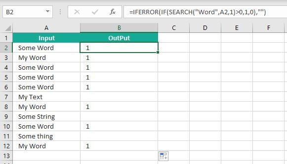
Search function will check for a given word in the required cell and return it’s position. We can use If function to check if the value is greater than 0 and assign a given value (example: 1) in the cell. search function returns #Value if there is no match found in the cell, we can handle this using IFERROR function.
Count If Cell Contains Text
We can check If Cell Contains Text Then COUNT. Here is the Excel formula to Count if a Cell contains Text. You can count the number of cells containing specific text.
The formula will Sum the values in Column B if the cells of Column A contains the given text.
Count If Cell Contains Partial Text
We can count the cells based on partial match criteria. The following Excel formula Counts if a Cell contains Partial Text.
- We can use the CountIf Function to Count the Cells if they contains given String
- Wild-card operators helps to make the CountIf to check for the Partial String
- Put Your Text between two asterisk symbols (*YourText*) to make the criteria to find any where in the given Cell
- Add Asterisk symbol at end of your text (YourText*) to make the criteria to find your text beginning of given Cell
- Place Asterisk symbol at beginning of your text (*YourText) to make the criteria to find your text end of given Cell
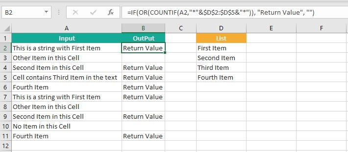
If Cell contains text from list then return value
Here is the Excel Formula to check if cell contains text from list then return value. We can use COUNTIF and OR function to check the array of values in a Cell and return the given Value. Here is the formula to check the list in range D2:D5 and check in Cell A2 and return value in B2.
If Cell Contains Text Then SUM
Following is the Excel formula to Sum if a Cell contains Text. You can total the cell values if there is given string in the Cell. Here is the example to sum the column B values based on the values in another Column.
The formula will Sum the values in Column B if the cells of Column A contains the given text.

Sum If Cell Contains Partial Text
Use SumIfs function to Sum the cells based on partial match criteria. The following Excel formula Sums the Values if a Cell contains Partial Text.
- SUMIFS Function will Sum the Given Sum Range
- We can specify the Criteria Range, and wild-card expression to check for the Partial text
- Put Your Text between two asterisk symbols (*YourText*) to Sum the Cells if the criteria to find any where in the given Cell
- Add Asterisk symbol at end of your text (YourText*) to Sum the Cells if the criteria to find your text beginning of given Cell
- Place Asterisk symbol at beginning of your text (*YourText) to Sum the Cells if criteria to find your text end of given Cell
VBA to check if Cell Contains Text
Here is the VBA function to find If Cells Contains Text using Excel VBA Macros.
If Cell Contains Partial Text VBA
We can use VBA to check if Cell Contains Text and Return Value. Here is the simple VBA code match the partial text. Excel VBA if Cell contains partial text macros helps you to use in your procedures and functions.
MsgBox CheckIfCellContainsPartialText(Cells(2, 1), “Region 1”)
End Sub
Function CheckIfCellContainsPartialText(ByVal cell As Range, ByVal strText As String) As Boolean
If InStr(1, cell.Value, strText) > 0 Then CheckIfCellContainsPartialText = True
End Function
- CheckIfCellContainsPartialText VBA Function returns true if Cell Contains Partial Text
- inStr Function will return the Match Position in the given string
If Cell Contains Text Then VBA MsgBox
Here is the simple VBA code to display message box if cell contains text. We can use inStr Function to search for the given string. And show the required message to the user.
If InStr(1, Cells(2, 1), “Region 3”) > 0 Then blnMatch = True
If blnMatch = True Then MsgBox “Cell Contains Text”
End Sub
- inStr Function will return the Match Position in the given string
- blnMatch is the Boolean variable becomes True when match string
- You can display the message to the user if a Range Contains Text
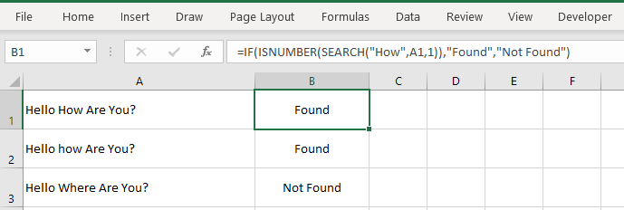
Which function returns true if cell a1 contains text?
You can use the Excel If function and Find function to return TRUE if Cell A1 Contains Text. Here is the formula to return True.
Which function returns true if cell a1 contains text value?
You can use the Excel If function with Find function to return TRUE if a Cell A1 Contains Text Value. Below is the formula to return True based on the text value.
Share This Story, Choose Your Platform!
7 Comments
-
Meghana
December 27, 2019 at 1:42 pm — ReplyHi Sir,Thank you for the great explanation, covers everything and helps use create formulas if cell contains text values.
Many thanks! Meghana!!
-
Max
December 27, 2019 at 4:44 pm — ReplyPerfect! Very Simple and Clear explanation. Thanks!!
-
Mike Song
August 29, 2022 at 2:45 pm — ReplyI tried this exact formula and it did not work.
-
Theresa A Harding
October 18, 2022 at 9:51 pm — Reply -
Marko
November 3, 2022 at 9:21 pm — ReplyHi
Is possible to sum all WA11?
(A1) WA11 4
(A2) AdBlue 1, WA11 223
(A3) AdBlue 3, WA11 32, shift 4
… and everything is in one column.
Thanks you very much for your help.
Sincerely Marko
-
Mike
December 9, 2022 at 9:59 pm — ReplyThank you for the help. The formula =OR(COUNTIF(M40,”*”&Vendors&”*”)) will give “TRUE” when some part of M40 contains a vendor from “Vendors” list. But how do I get Excel to tell which vendor it found in the M40 cell?
-
PNRao
December 18, 2022 at 6:05 am — ReplyPlease describe your question more elaborately.
Thanks!
-
© Copyright 2012 – 2020 | Excelx.com | All Rights Reserved
Page load link
To check if a cell contains specific text, use ISNUMBER and SEARCH in Excel. There’s no CONTAINS function in Excel.
1. To find the position of a substring in a text string, use the SEARCH function.

Explanation: «duck» found at position 10, «donkey» found at position 1, cell A4 does not contain the word «horse» and «goat» found at position 12.
2. Add the ISNUMBER function. The ISNUMBER function returns TRUE if a cell contains a number, and FALSE if not.

Explanation: cell A2 contains the word «duck», cell A3 contains the word «donkey», cell A4 does not contain the word «horse» and cell A5 contains the word «goat».
3. You can also check if a cell contains specific text, without displaying the substring. Make sure to enclose the substring in double quotation marks.

4. To perform a case-sensitive search, replace the SEARCH function with the FIND function.

Explanation: the formula in cell C3 returns FALSE now. Cell A3 does not contain the word «donkey» but contains the word «Donkey».
5. Add the IF function. The formula below (case-insensitive) returns «Found» if a cell contains specific text, and «Not Found» if not.

6. You can also use IF and COUNTIF in Excel to check if a cell contains specific text. However, the COUNTIF function is always case-insensitive.

Explanation: the formula in cell C2 reduces to =IF(COUNTIF(A2,»*duck*»),»Found»,»Not Found»). An asterisk (*) matches a series of zero or more characters. Visit our page about the COUNTIF function to learn all you need to know about this powerful function.
Author: Oscar Cronquist Article last updated on October 19, 2021

This article demonstrates different formulas based on if a cell contains a given text.
Formula in cell C3:
=B3=$E$3
The formula shown in the image above in cell C3 returns TRUE or FALSE based on a comparison between cell B3 and cell E3. The equal sign is a logical operator and returns boolean value TRUE or FALSE, it is not case sensitive.
Table of Contents
- If cell contains partial text
- Explaining formula
- If cell contains partial text — hardcoded asterisks
- Alternative function — SEARCH function
- If cell contains text then return value
- If cell contains text then add text in another cell
- If cell contains text then sum
- If cell contains text add 1
- Highlight cell if cell contains text (Link)
- Get Excel file
1. If cell contains partial text

The easiest way to check if a cell partially contains a specific text string is, in my opinion, the IF and COUNTIF function combined. The COUNTIF function allows you to count how many times a text string exists in a cell range.
Formula in cell D3:
=IF(COUNTIF(B3, C3), TRUE, FALSE)
The asterisk characters let you perform a wildcard match meaning that it matches any sequence of characters. Adding a beginning and ending asterisk to a text string allows you to check if a cell value contains a specific text string.
Back to top
1.1 Explaining formula in cell D3
Step 1 — Check if cell contains text condition
You can’t use asterisks with the equal sign to check if a cell contains a given text, however, the COUNTIF function can do that.
The COUNTIF function calculates the number of cells that is equal to a condition.
COUNTIF(range, criteria)
COUNTIF(B3, C3)
becomes
COUNTIF(«Green, red and blue»,»*red*»)
and returns 1.
Step 2 — Evaluate IF function
The IF function returns one value if the logical test is TRUE and another value if the logical test is FALSE.
IF(logical_test, [value_if_true], [value_if_false])
IF(COUNTIF(B3, C3), TRUE, FALSE)
becomes
IF(1, TRUE, FALSE)
The logical_test argument requires boolean values or their numerical equivalents. FALSE = 0 (zero), TRUE any number except zero.
Back to top
1.2 If cell contains partial text — hardcoded asterisks

Formula in cell D4:
=IF(COUNTIF(B4, «*»&C4&»*»), TRUE, FALSE)
You don’t have to add asterisks manually to your cell, you can easily build a formula that adds the asterisks automatically, demonstrated in cell D4. The ampersand & character lets you append the asterisks to the text string you want to use.
Note, if a text string is found twice in the same cell the COUNTIF function only returns 1. It counts cells not text strings.
Back to top
1. Alternative function — SEARCH function
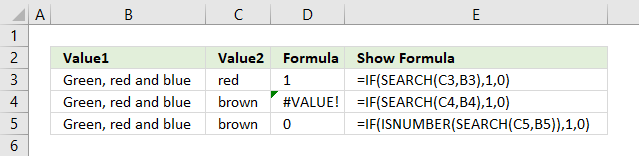
The SEARCH function returns the position of the character at which a specific text string is found. Luckily the IF function accepts any number as TRUE except 0 (zero), however, the SEARCH function returns an error #VALUE! if it can’t find the text string.
Formula in cell D5:
=IF(ISNUMBER(SEARCH(C5, B5)),1,0)
To avoid the error value I use the ISNUMBER function that returns TRUE if a number and FALSE if anything else, also formula errors.
Back to top
2. If cell contains text then return value

The formula in cell C3 checks if cell B3 contains the condition specified in cell E3. It returns the value if TRUE and a blank cell if FALSE.
Formula in cell C3:
=IF(COUNTIF(B3, «*»&$E$3&»*»), B3, «»)
Back to top
2.1 Explaining formula in cell C3
Step 1 — Concatenate strings
The asterisk is a wildcard character that matches 0 (zero) to any number of characters. The ampersand character concatenates strings in an Excel formula.
«*»&$E$3&»*»
becomes
«*»&»purple»&»*»
and returns «*purple*».
Step 2 — Check if cell contains string
The COUNTIF function calculates the number of cells that is equal to a condition.
COUNTIF(range, criteria)
COUNTIF(B3, «*»&$E$3&»*»)
becomes
COUNTIF(«Green, red and blue», «*purple*»)
and returns 0 (zero). Purple is not found in cell B3.
Step 3 — Return value if TRUE
The IF function returns one value if the logical test is TRUE and another value if the logical test is FALSE.
IF(logical_test, [value_if_true], [value_if_false])
IF(COUNTIF(B3, «*»&$E$3&»*»), B3, «»)
becomes
IF(0, B3, «»)
and returns «» in cell C3.
Back to top
3. If cell contains text then add text from another cell

The formula in cell C3 checks if cell B3 contains the condition specified in cell E3. It returns the value concatenated with a value on the same row from column if TRUE and a blank cell if FALSE.
Formula in cell C3:
=IF(COUNTIF(B3, «*»&$F$3&»*»), B3&C3, «»)
Back to top
3.1 Explaining formula in cell C4
Step 1 — Concatenate strings
The asterisk is a wildcard character that matches 0 (zero) to any number of characters. The ampersand character concatenates strings in an Excel formula.
«*»&$E$3&»*»
becomes
«*»&»purple»&»*»
and returns «*purple*».
Step 2 — Check if cell contains string
The COUNTIF function calculates the number of cells that is equal to a condition.
COUNTIF(range, criteria)
COUNTIF(B4, «*»&$E$3&»*»)
becomes
COUNTIF(«Black, purple, white», «*purple*»)
and returns 1. Purple is found in cell B4.
Step 3 — Return concatenated value if TRUE
The IF function returns one value if the logical test is TRUE and another value if the logical test is FALSE.
IF(logical_test, [value_if_true], [value_if_false])
IF(COUNTIF(B4, «*»&$E$3&»*»), B4&C4, «»)
becomes
IF(0, B4&C4, «»)
becomes
IF(0, «Black, purple, white»&»#11», «»)
and returns «Black, purple, white#11» in cell D4.
Back to top
4. If cell contains text then sum

The formula in cell F3 checks if cells in column B contain the condition specified in cell E3 and sums the corresponding values in column C.
Formula in cell C3:
=SUM(ISNUMBER(SEARCH(E3, B3:B6))*C3:C6)
Back to top
4.1 Explaining formula in cell C4
Step 1 — Search for string
The SEARCH function returns a number representing the position of character at which a specific text string is found reading left to right. It is not a case-sensitive search.
SEARCH(find_text,within_text, [start_num])
SEARCH(E3, B3:B6)
becomes
SEARCH(«North», {«North, South»; «South, East»; «West, North, South»; «South, West»})
and returns {1; #VALUE!; 7; #VALUE!}.
Step 2 — Check if value in array is an error
The ISNUMBER function checks if a value is a number, returns TRUE or FALSE.
ISNUMBER(SEARCH(E3, B3:B6))
becomes
ISNUMBER({1; #VALUE!; 7; #VALUE!})
and returns {TRUE; FALSE; TRUE; FALSE}.
Step 3 — Multiply corresponding numbers
The asterisk lets you multiply numbers in an Excel formula. We are multiplying boolean values in this example.
ISNUMBER(SEARCH(E3, B3:B6))*C3:C6
becomes
{TRUE; FALSE; TRUE; FALSE}*{10; 15; 6; 2}
TRUE equals 1 and FALSE equals 0 (zero).
{TRUE; FALSE; TRUE; FALSE}*{10; 15; 6; 2}
and returns {10; 0; 6; 0}.
Step 4 — Sum numbers
The SUM function adds numbers and returns a total.
SUM(ISNUMBER(SEARCH(E3, B3:B6))*C3:C6)
becomes
SUM({10; 0; 6; 0})
and returns 16 in cell F3.
Back to top
5. If cell contains text add 1

The formula in cell C3 counts cells containing the given text string in cell E3.
Formula in cell C3:
=IF(COUNTIF(B3,»*»&$E$3&»*»),1+MAX($C$2:C2),»»)
Back to top
5.1 Explaining formula in cell C3
Step 1 — Concatenate strings
The asterisk is a wildcard character that matches 0 (zero) to any number of characters. The ampersand character concatenates strings in an Excel formula.
«*»&$E$3&»*»
becomes
«*»&»North»&»*»
and returns «*North*».
Step 2 — Check if cell contains given string
The COUNTIF function calculates the number of cells that is equal to a condition.
COUNTIF(range, criteria)
COUNTIF(B3,»*»&$E$3&»*»)
becomes
COUNTIF(«North, South», «*North*»)
and returns 1.
Step 3 — Calculate count
The MAX function returns the largest number from a cell range or array.
Reference $C$2:C2 contains both absolute and relative cell references which makes it grow when the cell is copied to cells below.
1+MAX($C$2:C2)
becomes
1+0
and returns 1.
Step 4 — Show count if corresponding cell contains given string
The IF function returns one value if the logical test is TRUE and another value if the logical test is FALSE.
IF(logical_test, [value_if_true], [value_if_false])
IF(COUNTIF(B3,»*»&$E$3&»*»),1+MAX($C$2:C2),»»)
becomes
IF(C1,1+MAX($C$2:C2),»»)
becomes
IF(C1, 1, «»)
and returns 1.
Back to top
6. Get Excel *.xlsx file
Back to top
Getting IF Function to Work for Partial Text Match
In the dataset below, we want to write a formula in column B that will search the text in column A. Our formula will search the column A text for the text sequence “AT” and if found display “AT” in column B.

It doesn’t matter where the letters “AT” occur in the column A text, we need to see “AT” in the adjacent cell of column B. If the letters “AT” do not occur in the column A text, the formula in column B should display nothing.
Searching for Text with the IF Function
Let’s begin by selecting cell B5 and entering the following IF formula.
=IF(A5="*AT*","AT","")
Notice the formula returns nothing, even though the text in cell A5 contains the letter sequence “AT”.
The reason it fails is that Excel doesn’t work well when using wildcards directly after an equals sign in a formula.

Any function that uses an equals sign in a logical test does not like to use wildcards in this manner.
“But what about the SUMIFS function?”, I hear you saying.
If you examine a SUMIFS function, the wildcards don’t come directly after the equals sign; they instead come after an argument. As an example:
=SUMIFS($C$4:$C$18,$A$4:$A$18,"*AT*")The wildcard usage does not appear directly after an equals sign.
SEARCH Function to the Rescue
The first thing we need to understand is the syntax of the SEARCH function. The syntax is as follows:
SEARCH(find_text, within_text, [start_num])
- find_text – is a required argument that defines the text you are searching for.
- within_text – is a required argument that defines the text in which you want to search for the value defined in the find_text
- Start_num – is an option argument that defines the character number/position in the within_text argument you wish to start searching. If omitted, the default start character position is 1 (the first character on the left of the text.)
To see if the search function works properly on its own, lets perform a simple test with the following formula.
=SEARCH("AT",A5)
We are returned a character position which the letters “AT” were discovered by the SEARCH function. The first SEARCH found the letters “AT” beginning in the 1st character position of the text. The next discovery was in the 5th character position, and the last discovery was in the 4th character position.
The “#VALUE!” responses are the SEARCH function’s way of letting us know that the letters “AT” were not found in the search text.
We can use this new information to determine if the text “AT” exists in the companion text strings. If we see any number as a response, we know “AT” exists in the text string. If we receive an error response, we know the text “AT” does not exist in the text string.
NOTE: The SEARCH function is NOT case-sensitive. A search for the letters “AT” would find “AT”, “At”, “aT”, and “at”. If you wish to search for text and discriminate between different cases (case-sensitive), use the FIND function. The FIND function works the same as SEARCH, but with the added behavior of case-sensitivity.
Turning Numbers into Decisions
An interesting function in Excel is the ISNUMBER function. The purpose of the ISNUMBER function is to return “True” if something is a number and “False” if something is not a number. The syntax is as follows:
ISNUMBER(value)
- value – is a required argument that defines the data you are examining. The value can refer to a cell, a formula, or a name that refers to a cell, formula, or value.
Let’s add the ISNUMBER function to the logic of our previous SEARCH function.
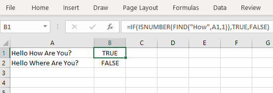
=ISNUMBER(SEARCH("AT",A5))
Any cell that contained a numeric response is now reading “True” and any cell that contained an error is now reading “False”.
We are now able to use the ISNUMBER/SEARCH functions as our wildcard statement in the original IF function.
=IF(ISNUMBER(SEARCH("AT",A5)),"AT","")
This is a great way to perform logical tests in functions that do not allow for wildcards.
Let’s see another scenario
Suppose we want to search for two different sets of text (“AT” or “DE”) and return the word “Europe” if either of these text strings are discovered in the searched text. We will combine the original formula with an OR function to search for multiple text strings.
=IF(OR(ISNUMBER(SEARCH("AT",A5)),ISNUMBER(SEARCH("DE",A5))),
"Europe","")
Practice Workbook
Feel free to Download the Workbook HERE.
![]()
Published on: June 2, 2019
Last modified: March 29, 2023


Leila Gharani
I’m a 5x Microsoft MVP with over 15 years of experience implementing and professionals on Management Information Systems of different sizes and nature.
My background is Masters in Economics, Economist, Consultant, Oracle HFM Accounting Systems Expert, SAP BW Project Manager. My passion is teaching, experimenting and sharing. I am also addicted to learning and enjoy taking online courses on a variety of topics.