
The IF function allows you to make a logical comparison between a value and what you expect by testing for a condition and returning a result if that condition is True or False.
-
=IF(Something is True, then do something, otherwise do something else)
But what if you need to test multiple conditions, where let’s say all conditions need to be True or False (AND), or only one condition needs to be True or False (OR), or if you want to check if a condition does NOT meet your criteria? All 3 functions can be used on their own, but it’s much more common to see them paired with IF functions.
Use the IF function along with AND, OR and NOT to perform multiple evaluations if conditions are True or False.
Syntax
-
IF(AND()) — IF(AND(logical1, [logical2], …), value_if_true, [value_if_false]))
-
IF(OR()) — IF(OR(logical1, [logical2], …), value_if_true, [value_if_false]))
-
IF(NOT()) — IF(NOT(logical1), value_if_true, [value_if_false]))
|
Argument name |
Description |
|
|
logical_test (required) |
The condition you want to test. |
|
|
value_if_true (required) |
The value that you want returned if the result of logical_test is TRUE. |
|
|
value_if_false (optional) |
The value that you want returned if the result of logical_test is FALSE. |
|
Here are overviews of how to structure AND, OR and NOT functions individually. When you combine each one of them with an IF statement, they read like this:
-
AND – =IF(AND(Something is True, Something else is True), Value if True, Value if False)
-
OR – =IF(OR(Something is True, Something else is True), Value if True, Value if False)
-
NOT – =IF(NOT(Something is True), Value if True, Value if False)
Examples
Following are examples of some common nested IF(AND()), IF(OR()) and IF(NOT()) statements. The AND and OR functions can support up to 255 individual conditions, but it’s not good practice to use more than a few because complex, nested formulas can get very difficult to build, test and maintain. The NOT function only takes one condition.

Here are the formulas spelled out according to their logic:
|
Formula |
Description |
|---|---|
|
=IF(AND(A2>0,B2<100),TRUE, FALSE) |
IF A2 (25) is greater than 0, AND B2 (75) is less than 100, then return TRUE, otherwise return FALSE. In this case both conditions are true, so TRUE is returned. |
|
=IF(AND(A3=»Red»,B3=»Green»),TRUE,FALSE) |
If A3 (“Blue”) = “Red”, AND B3 (“Green”) equals “Green” then return TRUE, otherwise return FALSE. In this case only the first condition is true, so FALSE is returned. |
|
=IF(OR(A4>0,B4<50),TRUE, FALSE) |
IF A4 (25) is greater than 0, OR B4 (75) is less than 50, then return TRUE, otherwise return FALSE. In this case, only the first condition is TRUE, but since OR only requires one argument to be true the formula returns TRUE. |
|
=IF(OR(A5=»Red»,B5=»Green»),TRUE,FALSE) |
IF A5 (“Blue”) equals “Red”, OR B5 (“Green”) equals “Green” then return TRUE, otherwise return FALSE. In this case, the second argument is True, so the formula returns TRUE. |
|
=IF(NOT(A6>50),TRUE,FALSE) |
IF A6 (25) is NOT greater than 50, then return TRUE, otherwise return FALSE. In this case 25 is not greater than 50, so the formula returns TRUE. |
|
=IF(NOT(A7=»Red»),TRUE,FALSE) |
IF A7 (“Blue”) is NOT equal to “Red”, then return TRUE, otherwise return FALSE. |
Note that all of the examples have a closing parenthesis after their respective conditions are entered. The remaining True/False arguments are then left as part of the outer IF statement. You can also substitute Text or Numeric values for the TRUE/FALSE values to be returned in the examples.
Here are some examples of using AND, OR and NOT to evaluate dates.

Here are the formulas spelled out according to their logic:
|
Formula |
Description |
|---|---|
|
=IF(A2>B2,TRUE,FALSE) |
IF A2 is greater than B2, return TRUE, otherwise return FALSE. 03/12/14 is greater than 01/01/14, so the formula returns TRUE. |
|
=IF(AND(A3>B2,A3<C2),TRUE,FALSE) |
IF A3 is greater than B2 AND A3 is less than C2, return TRUE, otherwise return FALSE. In this case both arguments are true, so the formula returns TRUE. |
|
=IF(OR(A4>B2,A4<B2+60),TRUE,FALSE) |
IF A4 is greater than B2 OR A4 is less than B2 + 60, return TRUE, otherwise return FALSE. In this case the first argument is true, but the second is false. Since OR only needs one of the arguments to be true, the formula returns TRUE. If you use the Evaluate Formula Wizard from the Formula tab you’ll see how Excel evaluates the formula. |
|
=IF(NOT(A5>B2),TRUE,FALSE) |
IF A5 is not greater than B2, then return TRUE, otherwise return FALSE. In this case, A5 is greater than B2, so the formula returns FALSE. |

Using AND, OR and NOT with Conditional Formatting
You can also use AND, OR and NOT to set Conditional Formatting criteria with the formula option. When you do this you can omit the IF function and use AND, OR and NOT on their own.
From the Home tab, click Conditional Formatting > New Rule. Next, select the “Use a formula to determine which cells to format” option, enter your formula and apply the format of your choice.

Using the earlier Dates example, here is what the formulas would be.

|
Formula |
Description |
|---|---|
|
=A2>B2 |
If A2 is greater than B2, format the cell, otherwise do nothing. |
|
=AND(A3>B2,A3<C2) |
If A3 is greater than B2 AND A3 is less than C2, format the cell, otherwise do nothing. |
|
=OR(A4>B2,A4<B2+60) |
If A4 is greater than B2 OR A4 is less than B2 plus 60 (days), then format the cell, otherwise do nothing. |
|
=NOT(A5>B2) |
If A5 is NOT greater than B2, format the cell, otherwise do nothing. In this case A5 is greater than B2, so the result will return FALSE. If you were to change the formula to =NOT(B2>A5) it would return TRUE and the cell would be formatted. |
Note: A common error is to enter your formula into Conditional Formatting without the equals sign (=). If you do this you’ll see that the Conditional Formatting dialog will add the equals sign and quotes to the formula — =»OR(A4>B2,A4<B2+60)», so you’ll need to remove the quotes before the formula will respond properly.
Need more help?

See also
You can always ask an expert in the Excel Tech Community or get support in the Answers community.
Learn how to use nested functions in a formula
IF function
AND function
OR function
NOT function
Overview of formulas in Excel
How to avoid broken formulas
Detect errors in formulas
Keyboard shortcuts in Excel
Logical functions (reference)
Excel functions (alphabetical)
Excel functions (by category)
Purpose
Test multiple conditions with OR
Return value
TRUE if any arguments evaluate TRUE; FALSE if not.
Usage notes
The OR function returns TRUE if any given argument evaluates to TRUE, and returns FALSE only if all supplied arguments evaluate to FALSE. The OR function can be used as the logical test inside the IF function to avoid nested IFs, and can be combined with the AND function.
The OR function is used to check more than one logical condition at the same time, up to 255 conditions, supplied as arguments. Each argument (logical1, logical2, etc.) must be an expression that returns TRUE or FALSE or a value that can be evaluated as TRUE or FALSE. The arguments provided to the OR function can be constants, cell references, arrays, or logical expressions.
The purpose of the OR function is to evaluate more than one logical test at the same time and return TRUE if any result is TRUE. For example, if A1 contains the number 50, then:
=OR(A1>0,A1>75,A1>100) // returns TRUE
=OR(A1<0,A1=25,A1>100) // returns FALSE
The OR function will evaluate all values supplied and return TRUE if any value evaluates to TRUE. If all logicals evaluate to FALSE, the OR function will return FALSE. Note: Excel will evaluate any number except zero (0) as TRUE.
Both the AND function and the OR function will aggregate results to a single value. This means they can’t be used in array operations that need to deliver an array of results. To work around this limitation, you can use Boolean logic. For more information, see: Array formulas with AND and OR logic.
Examples
For example, to test if the value in A1 OR the value in B1 is greater than 75, use the following formula:
=OR(A1>75,B1>75)
OR can be used to extend the functionality of functions like the IF function. Using the above example, you can supply OR as the logical_test for an IF function like so:
=IF(OR(A1>75,B1>75), "Pass", "Fail")
This formula will return «Pass» if the value in A1 is greater than 75 OR the value in B1 is greater than 75.
Array form
If you enter OR as an array formula, you can test all values in a range against a condition. For example, this array formula will return TRUE if any cell in A1:A100 is greater than 15:
=OR(A1:A100>15)
Note: In Legacy Excel, this is an array formula and must be entered with control + shift + enter.
Notes
- Each logical condition must evaluate to TRUE or FALSE, or be arrays or references that contain logical values.
- Text values or empty cells supplied as arguments are ignored.
- The OR function will return #VALUE if no logical values are found
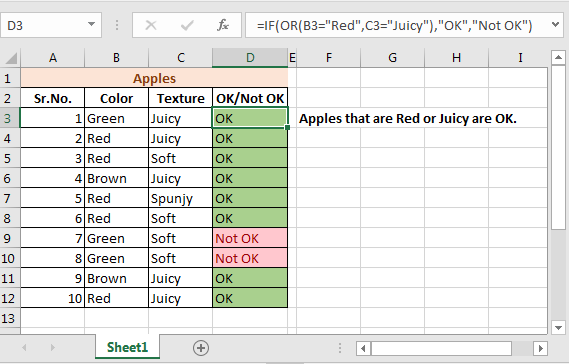
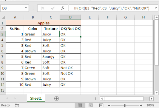
A fruit seller is selling apples. You will buy apples only if they are Red or Juicy. If an apple is not Red nor Juicy, you will not buy it.
Here we have two conditions and at least one of them need to be true to make you happy. Let’s write an IF OR formula for this in Excel 2016.
Implementation of IF with OR
Generic Formula
=IF(OR(condition1, condition2,…),value if true, value if false)
Example
Let’s consider the example we discussed in the beginning.
We have this table of apple’s colour and type.
If the colour is “Red” or type is “Juicy” then write OK in column D. If the color is not “Red”, nor the type is “Juicy” then type Not OK.

Write this IF OR formula in D2 column and drag it down.
=IF(OR(B3=»Red»,C3=»Juicy»),»OK»,»Not OK»)
And you can see now that only apples that are Red or Juicy are marked OK.
How It Works
IF Statement : You know how IF function in Excel works. It takes a boolean expression as first argument and returns one expression if TRUE and another if FALSE. Learn more about The Excel IF function.
=IF(TRUE or FALSE, statement if True, statement if false)
OR Function: Checks multiple conditions. Returns TRUE only if at least one of the conditions is TRUE else returns FALSE.
=OR(condition1, condition2,….) ==> TRUE/FALSE
In the end, OR function provides IF function TRUE or FALSE argument and based on that IF prints the result.
Alternate Solution:
Another way to do this is to use nested IFs for Multiple Conditions.
=IF(B3=»Red», “OK”, IF(C3=»Juicy»,”OK”,”Not OK”),”Not OK”)
Nested IF is good when we want different results but not when only one result. It will work but for multiple conditions, it will make your excel formula too long.
So here we learned about how to use IF with OR to check multiple conditions and show results if at least one of all conditions is TRUE. But what if you want to show results only if all condition is true. We will use AND function with IF in excel to do so.
Related Articles:
Excel OR function
Excel AND Function
IF with AND Function in Excel
Excel TRUE Function
Excel NOT function
IF not this or that in Microsoft Excel
IF with AND and OR function in Excel
Popular Articles:
The VLOOKUP Function in Excel
COUNTIF in Excel 2016
How to Use SUMIF Function in Excel
What is IF Function in Excel?
IF function in Excel evaluates whether a given condition is met and returns a value depending on whether the result is “true” or “false”. It is a conditional function of Excel, which returns the result based on the fulfillment or non-fulfillment of the given criteria.
For example, the IF formula in Excel can be applied as follows:
“=IF(condition A,“value B”,“value C”)”
The IF excel function returns “value B” if condition A is met and returns “value C” if condition A is not met.
It is often used to make logical interpretations which help in decision-making.
Table of contents
- What is IF Function in Excel?
- Syntax of the IF Excel Function
- How to Use IF Function in Excel?
- Example #1
- Example #2
- Example #3
- Example #4
- Example #5
- Guidelines for the Multiple IF Statements
- Frequently Asked Question
- IF Excel Function Video
- Recommended Articles
Syntax of the IF Excel Function
The syntax of the IF function is shown in the following image:

The IF excel function accepts the following arguments:
- Logical_test: It refers to the condition to be evaluated. The condition can be a value or a logical expression.
- Value_if_true: It is the value returned as a result when the condition is “true”.
- Value_if_false: It is the value returned as a result when the condition is “false”.
In the formula, the “logical_test” is a required argument, whereas the “value_if_true” and “value_if_false” are optional arguments.
The IF formula uses logical operators to evaluate the values in a range of cells. The following table shows the different logical operatorsLogical operators in excel are also known as the comparison operators and they are used to compare two or more values, the return output given by these operators are either true or false, we get true value when the conditions match the criteria and false as a result when the conditions do not match the criteria.read more and their meaning.
| Operator | Meaning |
|---|---|
| = | Equal to |
| > | Greater than |
| >= | Greater than or equal to |
| < | Less than |
| <= | Less than or equal to |
| <> | Not equal to |
How to Use IF Function in Excel?
Let us understand the working of the IF function with the help of the following examples in Excel.
You can download this IF Function Excel Template here – IF Function Excel Template
Example #1
If there is no oxygen on a planet, life is impossible. If oxygen is available on a planet, then life is possible. The following table shows a list of planets in column A and the information on the availability of oxygen in column B. We have to find the planets where life is possible, based on the condition of oxygen availability.

Let us apply the IF formula to cell C2 to find out whether life is possible on the planets listed in the table.
The IF formula is stated as follows:
“=IF(B2=“Yes”, “Life is Possible”, “Life is Not Possible”)
The succeeding image shows the IF formula applied to cell C2.

The subsequent image shows how the IF formula is applied to the range of cells C2:C5.

Drag the cells to view the output of all the planets.

The output in the below worksheet shows life is possible on the planet Earth.
Flow Chart of Generic IF Excel Function

The IF Function Flow Chart for Mars (Example #1)

The flow of IF function flowchart for Jupiter and Venus is the same as the IF function flowchart for Mars (Example #1).
The IF Function Flow Chart for Earth

Hence, the IF excel function allows making logical comparisons between values. The modus operandi of the IF function is stated as: If something is true, then do something; otherwise, do something else.
Example #2
The following table shows a list of years. We want to find out if the given year is a leap year or not.
A leap year has 366 days; the extra day is the 29th of February. The criteria for a leap year are stated as follows:
- The year will be exactly divisible by 4 and not exactly be divisible by 100 or
- The year will be exactly divisible by 400.

In this example, we will use the IF function along with the AND, OR, and MOD functions to find the leap years.
We use the MOD function to find a remainder after a dividend is divided by a divisor.
The AND functionThe AND function in Excel is classified as a logical function; it returns TRUE if the specified conditions are met, otherwise it returns FALSE.read more evaluates both the conditions of the leap years for the value “true”. The OR functionThe OR function in Excel is used to test various conditions, allowing you to compare two values or statements in Excel. If at least one of the arguments or conditions evaluates to TRUE, it will return TRUE. Similarly, if all of the arguments or conditions are FALSE, it will return FASLE.read more evaluates either of the condition for the value “true”.
We will apply the MOD function to the conditions as follows:
If MOD(year,4)=0 and MOD(year,100)<>(is not equal to) 0, then the year is a leap year.
or
If MOD(year,400)=0, then the year is a leap year; otherwise, the year is not a leap year.
The IF formula is stated as follows:
“=IF(OR(AND((MOD(year,4)=0),(MOD(year,100)<>0)),(MOD(year,400)=0)),“Leap Year”, “Not A Leap Year”)”
The argument “year” refers to a reference value.
The following images show the output of the IF formula applied in the range of cells.


The following image shows how the IF formula is applied to the range of cells B2:B18.

The succeeding table shows the years 1960, 2028, and 2148 as leap years and the remaining as non-leap years.

The result of the IF excel formula is displayed for the range of cells B2:B18 in the following image.

Example #3
The succeeding table shows a list of drivers and the directions they undertook to reach the destination. It is preceded by an image of the road intersection explaining the turns taken by the drivers and their destinations. The right turn leads to town B, and the left turn leads to town C. Identify the driver’s destination to town B and town C.
Road Intersection Image


Let us apply the IF excel function to find the destination. Here, the condition is mentioned as follows:
- If the driver turns right, he/she reaches town B.
- If the driver turns left, he/she reaches town C.
We use the following IF formula to find the destination:
“=IF(B2=“Left”, “Town C”, “Town B”)”
The succeeding image shows the output of the IF formula applied to cell C2.

Drag the cells to use the formula in the range C2:C11. Finally, we get the destinations of each driver for their turning movements.
The below image displays the IF formula applied to the range.

The output of the IF formula and the destinations are displayed in the succeeding image.

The result shows that six drivers reached town C, and the remaining four have reached town B.
Example #4
The following table shows a list of items and their inventory levels. We want to check if the specific item is available in the inventory or not using the IF function.

Let us list the name of items in column A and the number of items in column B. The list of data to be validated for the entire items list is shown in the cell E2 of the below image.

We use the Excel IF along with the VLOOKUP functionThe VLOOKUP excel function searches for a particular value and returns a corresponding match based on a unique identifier. A unique identifier is uniquely associated with all the records of the database. For instance, employee ID, student roll number, customer contact number, seller email address, etc., are unique identifiers.
read more to check the availability of the items in the inventory.
The VLOOKUP function looks up the values referring to the number of items, and the IF function will check whether the item number is greater than zero or not.
We will apply the following IF formula in the F2 cell:
“=IF(VLOOKUP(E2,A2:B11,2,0)=0, “Item Not Available”,“Item Available”)”
If the lookup value of an item is equal to 0, then the item is not available; else, the item is available.
The succeeding image shows the result of the IF formula in the cell F2.

Select “bat” in the E2 item cell to know whether the item is available or not in the inventory (as shown in the following image).

Example #5
The following table shows the list of students and their marks. The grade criteria are provided based on the marks obtained by the students. We want to find the grade of each student in the list.

We apply the Nested IF in Excel since we have multiple criteria to find and decide each student’s grade.
The Nesting of IF function uses the IF function inside another IF formula when multiple conditions are to be fulfilled.
The syntax of Nesting of IF function is stated as follows:
“=IF( condition1, value_if_true1, IF( condition2, value_if_true2, value_if_false2 ))”
The succeeding table represents the range of scores and the grades, respectively.

Let us apply the multiple IF conditions with AND function in the below-nested formula to find out the grade of the students:
“=IF((B2>=95),“A”,IF(AND(B2>=85,B2<=94),“B”,IF(AND(B2>=75,B2<=84),“C”,IF(AND(B2>=61,B2<=74),“D”,“F”))))”
The IF function checks the logical condition as shown in the formula below:
“=IF(logical_test, [value_if_true],[value_if_false])”
We will split the above-mentioned nested formula and check the IF statements as shown below:
First Logical Test: B2>=95
If the formula returns,
- Value_if_true, execute: “A” (Grade A) else(comma) enter value_if_false
- Value_if_false, then the formula finds another IF condition and enter IF condition
Second Logical Test: B2>=85(logical expression 1) and B2<=94(logical expression 2)
(We use AND function to check the multiple logical expressions as the two given conditions are to be evaluated for “true.”)
If the formula returns,
- Value_if_true, execute: “B” (Grade B) else(comma) enter value_if_false
- Value_if_false, then the formula finds another IF condition and enter IF condition
Third Logical Test: B2>=75(logical expression 1) and B2<=84(logical expression 2)
(We use AND function to check the multiple logical expressions as the two given conditions are to be evaluated for “true.”)
If the formula returns,
- Value_if_true, execute: “C” (Grade C) else(comma) enter value_if_false
- value_if_false, then the formula finds another IF condition and enter IF condition
Fourth Logical Test: B2>=61(logical expression 1) and B2<=74(logical expression 2)
(We use AND function to check the multiple logical expressions as the two given conditions are to be evaluated for “true.”)
If the formula returns,
- Value_if_true, execute: “D” (Grade D) else(comma) enter value_if_false
- Value_if_false, execute: “F” (Grade F)
- Finally, close the parenthesis.
The below image displays the output of the IF formula applied to the range.

The succeeding image shows the IF nested formula applied to the range.

The grades of the students are listed in the following table.

Guidelines for the Multiple IF Statements
The guidelines for the multiple IF statements are listed as follows:
- Use nested IF function to a limited extent as multiple IF statements require a great deal of thought to be accurate.
- Multiple IF statementsIn Excel, multiple IF conditions are IF statements that are contained within another IF statement. They are used to test multiple conditions at the same time and return distinct values. Additional IF statements can be included in the ‘value if true’ and ‘value if false’ arguments of a standard IF formula.read more require multiple parentheses (), which is often difficult to manage. Excel provides a way to check the color of each opening and closing parenthesis to avoid this situation. The last closing parenthesis color will always be black, denoting the end of the formula statement.
- Whenever we pass a string value for the arguments “value_if_true” and “value_if_false” or test a reference against a string value, enclose the string value in double quotes. Passing a string value without quotes will result in “#NAME?” error.
Frequently Asked Question
1. What is the IF function in Excel?
The Excel IF function is a logical function that checks the given criteria and returns one value for a “true” and another value for a “false” result.
The syntax of the IF function is stated as follows:
“=IF(logical_test, [value_if_true], [value_if_false])”
The arguments are as follows:
1. Logical_test – It refers to a value or condition that is tested.
2. Value_if_true – It is the value returned when the condition logical_test is “true.”
3. Value_if_false – It is the value returned when the condition logical_test is “false.”
The “logical_test” is a required argument, whereas the “value_if_true” and “value_if_false” are optional arguments.
2. How to use the IF Excel function with multiple conditions?
The IF Excel statement for multiple conditions is created by using multiple IF functions in a single formula.
The syntax of IF function with multiple conditions is stated as follows:
“=IF (condition 1_“true”, do something, IF (condition 2_“true”, do something, IF (condition 3_ “true”, do something, else do something)))”
3. How to use the function IFERROR in Excel?
IF Excel Function Video
Recommended Articles
This has been a guide to the IF function in Excel. Here we discuss how to use the IF function along with examples and downloadable templates. You may also look at these useful functions –
- What is the Logical Test in Excel?A logical test in Excel results in an analytical output, either true or false. The equals to operator, “=,” is the most commonly used logical test.read more
- “Not Equal to” in Excel“Not Equal to” argument in excel is inserted with the expression <>. The two brackets posing away from each other command excel of the “Not Equal to” argument, and the user then makes excel checks if two values are not equal to each other.read more
- Data Validation ExcelThe data validation in excel helps control the kind of input entered by a user in the worksheet.read more
Excel IF AND OR functions on their own aren’t very exciting, but mix them up with the IF Statement and you’ve got yourself a formula that’s much more powerful.
In this tutorial we’re going to take a look at the basics of the AND and OR functions and then put them to work with an IF Statement. If you aren’t familiar with IF Statements, click here to read that tutorial first.
IF Formula Builder
Our IF Formula Builder does the hard work of creating IF formulas.
You just need to enter a few pieces of information, and the workbook creates the formula for you.
AND Function
The AND function belongs to the logic family of formulas, along with IF, OR and a few others. It’s useful when you have multiple conditions that must be met.
In Excel language on its own the AND formula reads like this:
=AND(logical1,[logical2]....)
Now to translate into English:
=AND(is condition 1 true, AND condition 2 true (add more conditions if you want)
OR Function
The OR function is useful when you are happy if one, OR another condition is met.
In Excel language on its own the OR formula reads like this:
=OR(logical1,[logical2]....)
Now to translate into English:
=OR(is condition 1 true, OR condition 2 true (add more conditions if you want)
See, I did say they weren’t very exciting, but let’s mix them up with IF and put AND and OR to work.
IF AND Formula
First let’s set the scene of our challenge for the IF, AND formula:
In our spreadsheet below we want to calculate a bonus to pay the children’s TV personalities listed. The rules, as devised by my 4 year old son, are:
1) If the TV personality is Popular AND
2) If they earn less than $100k per year they get a 10% bonus (my 4 year old will write them an IOU, he’s good for it though).

In cell D2 we will enter our IF AND formula as follows:
In English first
=IF(Spider Man is Popular, AND he earns <$100k), calculate his salary x 10%, if not put "Nil" in the cell)
Now in Excel’s language:
=IF(AND(B2="Yes",C2<100),C2x$H$1,"Nil")
You’ll notice that the two conditions are typed in first, and then the outcomes are entered. You can have more than two conditions; in fact you can have up to 30 by simply separating each condition with a comma (see warning below about going overboard with this though).
IF OR Formula
Again let’s set the scene of our challenge for the IF, OR formula:
The revised rules, as devised by my 4 year old son, are:
1) If the TV personality is Popular OR
2) If they earn less than $100k per year they get a 10% bonus.

In cell D2 we will enter our IF OR formula as follows:
In English first
=IF(Spider Man is Popular, OR he earns <$100k), calculate his salary x 10%, if not put “Nil” in the cell)
Now in Excel’s language:
=IF(OR(B2="Yes",C2<100),C2x$H$1,"Nil")
Notice how a subtle change from the AND function to the OR function has a significant impact on the bonus figure.
Just like the AND function, you can have up to 30 OR conditions nested in the one formula, again just separate each condition with a comma.
Try other operators
You can set your conditions to test for specific text, as I have done in this example with B2=»Yes», just put the text you want to check between inverted comas “ ”.
Alternatively you can test for a number and because the AND and OR functions belong to the logic family, you can employ different tests other than the less than (<) operator used in the examples above.
Other operators you could use are:
- = Equal to
- > Greater Than
- <= Less than or equal to
- >= Greater than or equal to
- <> Less than or greater than
Warning: Don’t go overboard with nesting IF, AND, and OR’s, as it will be painful to decipher if you or someone else ever needs to update the formula in months or years to come.
Note: These formulas work in all versions of Excel, however versions pre Excel 2007 are limited to 7 nested IF’s.
Download the Workbook
Enter your email address below to download the sample workbook.
By submitting your email address you agree that we can email you our Excel newsletter.
Excel IF AND OR Practice Questions
IF AND Formula Practice
In the embedded Excel workbook below insert a formula (in the grey cells in column E), that returns the text ‘Yes’, when a product SKU should be reordered, based on the following criteria:
- If Stock on hand is less than 20,000 AND
- Demand level is ‘High’
If the above conditions are met, return ‘Yes’, otherwise, return ‘No’.
Tips for working with the embedded workbook:
- Use arrow keys to move around the worksheet when you can’t click on the cells with your mouse
- Use shortcut keys CTRL+C to copy and CTRL+V to paste
- Don’t forget to absolute cell references where applicable
- Do not enter anything in column F
- Double click to edit a cell
- Refresh the page to reset the embedded workbook
IF OR Formula Practice
In the embedded Excel workbook below insert a formula (in the grey cells in column E) that calculates the bonus due for each salesperson. A $500 bonus is paid if a salesperson meets either target in cells C24 and C25, otherwise they earn $0 bonus.
Want More Excel Formulas
Why not visit our list of Excel formulas. You’ll find a huge range all explained in plain English, plus PivotTables and other Excel tools and tricks. Enjoy 🙂
Logical functions are designed to test one or several conditions, and perform the actions prescribed for each of the two possible results. Such results can only be logical TRUE or FALSE.
Excel contains several logical functions such as IF, IFERROR, SUMIF, AND, OR, and others. The last two are not used in practice, as a rule, because the result of their calculations may be one of only two possible options (TRUE, FALSE). When combined with the IF function, they are able to significantly expand its functionality.
Examples of using formulas with IF, AND, OR functions in Excel
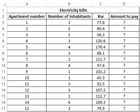
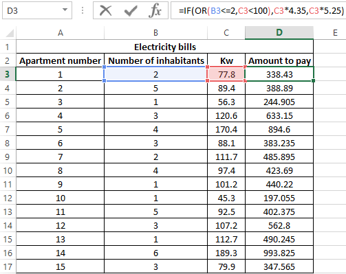
Example 1. When calculating the cost of the amount of consumed kW of electricity for subscribers, the following conditions are taken into account:
- If less than 3 people live in the apartment or less than 100 kW of electricity was consumed per month, the rate per 1 kW is 4.35$.
- In other cases, the rate for 1 kW is 5.25$.
Calculate the amount payable per month for several subscribers.
View source data table:
Perform the calculation according to the formula:
Argument Description:
- OR (B3<=2,C3<100) is a logical expression that verifies two conditions: do less than 3 people live in the apartment or does the total amount of energy consumed less than 100 kW? The result of the test will be TRUE if either of these two conditions is true;
- C3 * 4.35 — the amount to be paid, if the OR function returns TRUE;
- C3 * 5.25 is the amount to be paid if OR returns FALSE.
We stretch the formula for the remaining cells using the autocomplete function. The result of the calculation for each subscriber:
Using the AND function in the formula in the first argument in the IF function, we check the conformity of the values by two conditions at once.
Formula with IF and AVERAGE functions for selecting of values by conditions
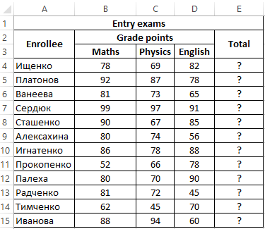
Example 2. Applicants entering the university for the specialty «mechanical engineer» are required to pass 3 exams in mathematics, physics and English. The maximum score for each exam is 100. The average passing score for 3 exams is 75, while the minimum score in physics must be at least 70 points, and in mathematics it is 80. Determine applicants who have successfully passed the exams.
View source table:
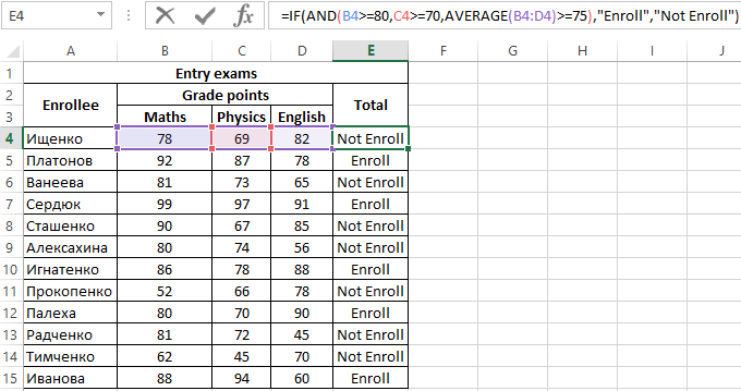
To determine the enrolled students use the formula:
Argument Description:
- AND(B4>=80,C4>=70,AVERAGE(B4:D4)>=75) — checked logical expressions according to the condition of the problem;
- «Enroll» — the result, if the function AND returned the value TRUE (all expressions represented as its arguments, as a result of the calculations returned the value TRUE);
- «Not Enroll» — the result if AND returned FALSE.
Using the autocomplete function (double-click on the cursor marker in the lower right corner), we get the rest of the results:
Formula with logical functions AND IF OR in excel
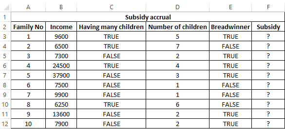
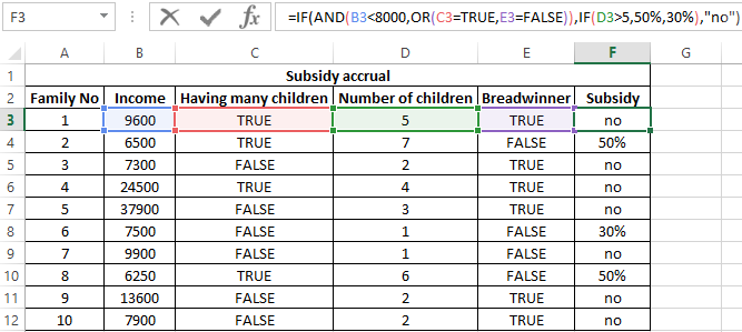
Example 3. Subsidies in the amount of 30% are charged to families with an average income below 8,000$, which are large or there is no main breadwinner. If the number of children is over 5, the amount of the subsidy is 50%. Determine who should receive subsidies and who should not.
View source table:
To check the criteria according to the condition of the problem, we write the formula:
Argument Description:
- AND(B3<8000,OR(C3=TRUE,E3=FALSE)) is the checked expression according to the condition of the problem. In this case, the AND function returns the TRUE value, if B3 <8000 is true and at least one of the expressions passed as arguments to the OR function also returns the TRUE value.
- The nested IF function performs a check on the number of children in the family, which rely on subsidies.
- If the main condition returned the result is FALSE, the main function IF returns the text string “no”.
Perform the calculation for the first family and stretch the formula to the remaining cells using the autocomplete function. Results:
Features of using logical functions IF, AND, OR in Excel
The IF function has the following syntax notation:
=IF(Logical_test,[ Value_if_True ],[ Value_if_False])
As you can see, by default, you can check only one condition, for example, is e3 more than 20? Using the IF function, this check can be done as follows:
=IF(EXP(3)>20,»more»,»less»)
As a result, the text string “more” will be returned. If we need to find out if any value belongs to the specified interval, we will need to compare this value with the upper and lower limits of the intervals, respectively. For example, is the result of calculating e3 in the range from 20 to 25? When using the IF function alone, you must enter the following entry:
=IF(EXP(3)>20,IF(EXP(3)<25,»belongs»,»does not belong»),»does not belong»)
We have a nested function IF as one of the possible results of the implementation of the main function IF, and therefore the syntax looks somewhat cumbersome. If you also need to know, for example, whether the square root e3 is equal to a numeric value from a fractional number range from 4 to 5, the final formula will look cumbersome and unreadable.
It is much easier to use as a condition a complex expression that can be written using AND and OR functions. For example, the above function can be rewritten as follows:
=IF(AND(EXP(3)>20,EXP(3)<25),»belongs»,»does not belong»)
The result of the execution of the AND expression (EXP(3)>20,EXP(3)<25) can be a logical value TRUE only if the result of checking each of the specified conditions is a logical value TRUE. In other words, the function AND allows you to test one, two or more hypotheses on their truth, and returns the result FALSE if at least one of them is incorrect.
Sometimes you want to know if at least one assumption is true. In this case, it is convenient to use the OR function, which performs the check of one or several logical expressions and returns a logical TRUE, if the result of the calculations of at least one of them is a logical TRUE. For example, you want to know if e3 is an integer or a number that is less than 100? To test this condition, you can use the following formula:
=IF(OR(MOD(EXP(3),1)<>0,EXP(3)<100),»true»,»false»)
The “<>” means inequality, that is, more or less than some value. In this case, both expressions return the value TRUE, and the result of the execution of the IF function is the text string «true.» However, if an OR test was performed (MOD(EXP (3),1)<>0,EXP(3)<20, while EXP(3) <20 will return FALSE, the result of the calculation of the IF function will not change, since MOD(EXP(3),1) <> 0 returns TRUE.
Download examples using the functions OR AND IF in Excel
In practice, often used bundles IF + AND, IF + OR, or all three functions at once. Consider examples of similar use of these functions.
When you work with data and formulas in Excel, you’re bound to encounter errors.
To handle errors, Excel has provided a useful function – the IFERROR function.
Before we get into the mechanics of using the IFERROR function in Excel, let’s first go through the different kinds of errors you can encounter when working with formulas.
Types of Errors in Excel
Knowing the errors in Excel will better equip you to identify the possible reason and the best way to handle these.
Below are the types of errors you might find in Excel.
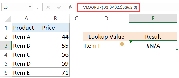
#N/A Error
This is called the ‘Value Not Available’ error.
You will see this when you use a lookup formula and it can’t find the value (hence Not Available).
Below is an example where I use the VLOOKUP formula to find the price of an item, but it returns an error when it can’t find that item in the table array.
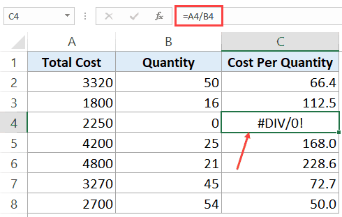
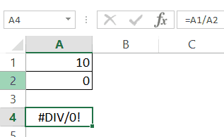
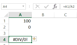
#DIV/0! Error
You’re likely to see this error when a number is divided by 0.
This is called the division error. In the below example, it gives a #DIV/0! error as the quantity value (the divisor in the formula) is 0.
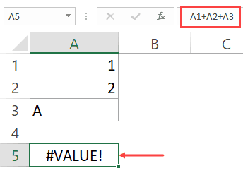
#VALUE! Error
The value error occurs when you use an incorrect data type in a formula.
For example, in the below example, when I try to add cells that have numbers and character A, it gives the value error.
This happens as you can only add numeric values, but instead, I tried adding a number with a text character.
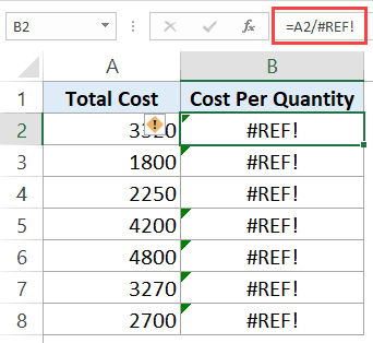
#REF! Error
This is called the reference error and you will see this when the reference in the formula is no longer valid. This could be the case when the formula refers to a cell reference and that cell reference does not exist (happens when you delete a row/column or worksheet that was referred to in the formula).
In the below example, while the original formula was =A2/B2, when I deleted Column B, all the references to it became #REF! and it also gave the #REF! error as the result of the formula.
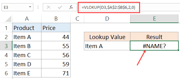
#NAME ERROR
This error is likely to a result of a misspelled function.
For example, if instead of VLOOKUP, you by mistake use VLOKUP, it will give a name error.
#NUM ERROR
Num error can occur if you try and calculate a very large value in Excel. For example, =187^549 will return a number error.
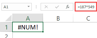
Another situation where you can get the NUM error is when you give a non-valid number argument to a formula. For example, if you’re calculating the Square Root if a number and you give a negative number as the argument, it will return a number error.
For example, in the case of Square Root function, if you give a negative number as the argument, it will return a number error (as shown below).
While I have shown only a couple of examples here, there can be many other reasons that can lead to errors in Excel. When you get errors in Excel, you can’t just leave it there. If the data is further used in calculations, you need to make sure the errors are handled the right way.
Excel IFERROR function is a great way to handle all types of errors in Excel.
Excel IFERROR Function – An Overview
Using the IFERROR function, you can specify what you want the formula to return instead of the error. If the formula does not return an error, then its own result is returned.
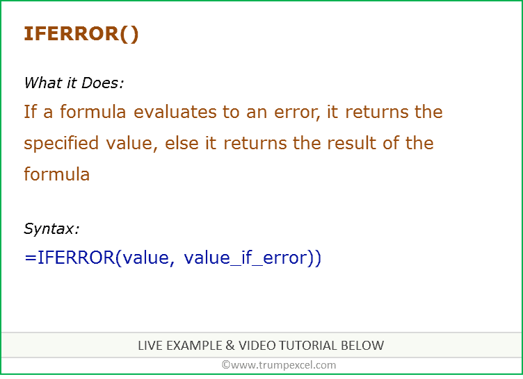
IFERROR Function Syntax
=IFERROR(value, value_if_error)
Input Arguments
- value – this is the argument that is checked for the error. In most cases, it is either a formula or a cell reference.
- value_if_error – this is the value that is returned if there is an error. The following error types evaluated: #N/A, #REF!, #DIV/0!, #VALUE!, #NUM!, #NAME?, and #NULL!.
Additional Notes:
- If you use “” as the value_if_error argument, the cell displays nothing in case of an error.
- If the value or value_if_error argument refers to an empty cell, it is treated as an empty string value by the Excel IFERROR function.
- If the value argument is an array formula, IFERROR will return an array of results for each item in the range specified in value.
Excel IFERROR Function – Examples
Here are three examples of using IFERROR function in Excel.
Example 1 – Return Blank Cell Instead of Error
If you have functions that may return an error, you can wrap it within the IFERROR function and specify blank as the value to return in case of an error.
In the example shown below, the result in D4 is the #DIV/0! error as the divisor is 0.
In this case, you can use the following formula to return blank instead of the ugly DIV error.
=IFERROR(A1/A2,””)
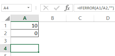
This IFERROR function would check whether the calculation leads to an error. If it does, it simply returns a blank as specified in the formula.
Here, you can also specify any other string or formula to display instead of the blank.
For example, the below formula would return the text “Error”, instead of the blank cell.
=IFERROR(A1/A2,”Error”)

Note: If you are using Excel 2003 or a prior version, you will not find the IFERROR function in it. In such cases, you need to use the combination of IF function and ISERROR function.
Example 2 – Return ‘Not Found’ when VLOOKUP Can’t Find a Value
When you use the Excel VLOOKUP Function, and it can’t find the lookup value in the specified range, it would return the #N/A error.
For example, below is a data set of student names and their marks. I have used the VLOOKUP function to fetch the marks of three students (in D2, D3, and D4).
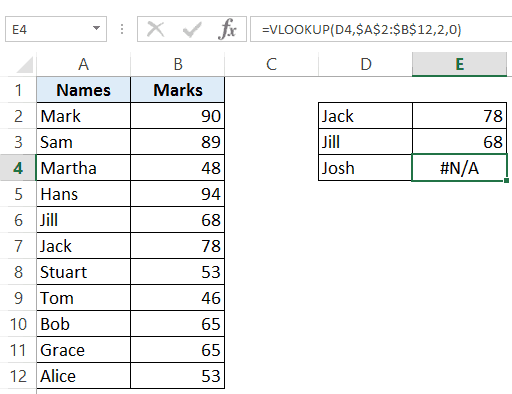
While the VLOOKUP formula in the above example finds the names of first two students, it can’t find Josh’s name on the list and hence it returns the #N/A error.
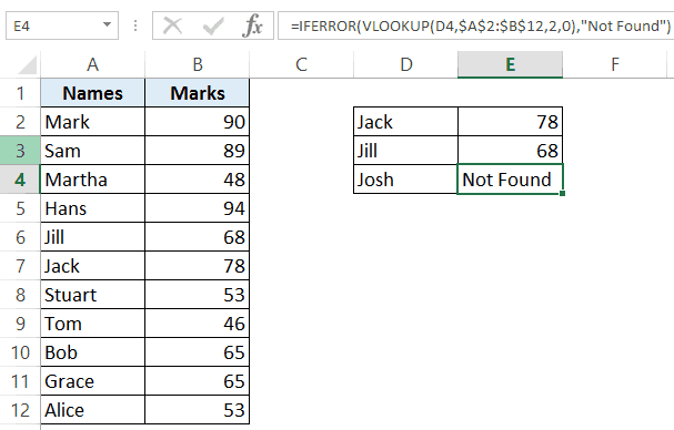
Here, we can use the IFERROR function to return a blank or some meaningful text instead of the error.
Below is the formula that will return ‘Not Found’ instead of the error.
=IFERROR(VLOOKUP(D2,$A$2:$B$12,2,0),”Not Found”)
Note that you can also use IFNA instead of IFERROR with VLOOKUP. While IFERROR would treat all kinds of error values, IFNA would only work on the #N/A errors and wouldn’t work with other errors.
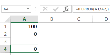
Example 3 – Return 0 in case of an Error
If you don’t specify the value to return by IFERROR in the case of an error, it would automatically return 0.
For example, if I divide 100 with 0 as shown below, it would return an error.
However, if I use the below IFERROR function, it would return a 0 instead. Note that you still need to use a comma after the first argument.
Example 4 – Using Nested IFERROR with VLOOKUP
Sometimes when using VLOOKUP, you may have to look through the fragmented table of arrays. For example, suppose you have the sales transaction records in 2 separate worksheets and you want to look-up an item number and see it’s value.
Doing this requires using nested IFERROR with VLOOKUP.
Suppose you have a dataset as shown below:
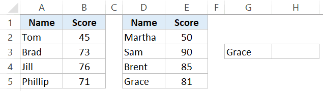
In this case, to find the score for Grace, you need to use the below nested IFERROR formula:
=IFERROR(VLOOKUP(G3,$A$2:$B$5,2,0),IFERROR(VLOOKUP(G3,$D$2:$E$5,2,0),"Not Found"))
This kind of formula nesting ensure that you get the value from either of the table and any error returned is handled.
Note that in case the tables are on the same worksheet, however, in a real-life example, it likely to be on different worksheets.
Excel IFERROR Function – VIDEO
Related Excel Functions:
- Excel AND Function.
- Excel OR Function.
- Excel NOT Function.
- Excel IF Function.
- Excel IFS Function.
- Excel FALSE Function.
- Excel TRUE Function.
You May Also Like the Following Excel Tutorials:
- Use IFERROR with VLOOKUP to Get Rid of #N/A Errors.
- Identify Errors Using Excel Formula Debugging.
IF function is undoubtedly one of the most important functions in excel. In general, IF statements give the desired intelligence to a program so that it can make decisions based on given criteria and, most importantly, decide the program flow.
In Microsoft Excel terminology, IF statements are also called «Excel IF-Then statements». IF function evaluates a boolean/logical expression and returns one value if the expression evaluates to ‘TRUE’ and another value if the expression evaluates to ‘FALSE’.
Definition of Excel IF Function
According to Microsoft Excel, IF function is defined as a formula which «checks whether a condition is met, returns one value if true and another value if false».
Syntax
Syntax of IF function in Excel is as follows:
=IF(logic_test, [value_if_true], [value_if_false])
'logic_test' (required argument) – Refers to the boolean expression or logical expression that needs to be evaluated.'value_if_true' (optional argument) – Refers to the value that will be returned by the IF function if the 'logic_test' evaluates to TRUE.'value_if_false' (optional argument) – Refers to the value that will be returned by the IF function if the 'logic_test' evaluates to FALSE.

Important Characteristics of IF Function in Excel
- To use the IF function, you need to provide the
'logic_test'or conditional statement mandatorily. - The arguments
'value_if_true'and'value_if_false'are optional, but you need to provide at least one of them. - The result of the IF statement can only be any one of the two given values (either it will be
'value_if_true'or'value_if_false'). Both values cannot be returned at the same time. - IF function throws a ‘#Name?’ error if the
'logic_test'or boolean expression you are trying to evaluate is invalid. - Nesting of IF statements is possible, but Excel only allows this to 64 levels. Nesting of IF statement means using one if statement within another.
Comparison Operators That Can Be Used With IF Statements
Following comparison operators can be used within the 'logic_test' argument of the IF function:
- = (equal to)
- <> (not equal to)
- < (less than)
- > (greater than)
- >= (greater than or equal to)
- <= (less than or equal to)
- Apart from these, you can also use any other function that returns a boolean result (either ‘true’ or ‘false’). For example – ISBLANK, ISERROR, ISEVEN, ISODD, etc
Now, let’s see some simple examples to use these comparison operators within the IF Function:
Simple Examples of Excel IF Statement
Now, let’s try to see a simple example of the Excel IF function:
Example 1: Using ‘equal to’ comparison operator within the IF function
In this example, we have a list of colors, and we aim to find the ‘Blue’ color. If we are able to find the ‘Blue’ color, then in the adjacent cell, we need to assign a ‘Yes’; otherwise, assign a ‘No’.

So, the formula would be:
=IF(A2="Blue", "No", "Yes")
This suggests that if the value present in cell A2 is ‘Blue’, then return a ‘Yes’; otherwise, return a ‘No’.
If we drag this formula down to all the rows, we will find that it returns ‘Yes’ for the cells with the value ‘Blue’ for all others; it would result in ‘No’.
Example 2: Using ‘not equal to’ comparison operator within the IF function.
Let’s take example 1, and understand how we can reverse the logic and use a ‘not equal to’ operator to construct the formula so that it still results in ‘Yes’ for ‘Blue’ color and ‘No’ for any other text.

So the formula would be:
=IF(A2<>"Blue", "No", "Yes")
This suggests that if the value at A2 is not equal to ‘Blue’, then return a ‘No’; otherwise, return a ‘Yes’.
When dragged down to all the below rows, this formula would find all the cells (from A2 to A8) where the value is not ‘Blue’ and marks a ‘No’ against them. Otherwise, it marks a ‘Yes’ in the adjacent cells.
Example 3: Using ‘less than’ operator within the IF function.
In this example, we have scores of some students, along with their names. We want to assign either «Pass» or «Fail» against each student in the result column.

Based on our criteria, the passing score is 50 or more.
For this, we can use the IF function as:
=IF(B2<50,"Fail","Pass")
This suggests that if the value at B2, i.e., 37, is less than 50, then return «Fail»; otherwise, return «Pass».
As 37 is less than 50 so the result will be «Fail».
We can drag the above-given formula for the rest of the cells below and the result would be correct.
Example 4: Using ‘greater than or equal to’ operator within the IF statement.
Let’s take example 3 and see how we can reverse the logic and use a ‘greater than or equal to’ operator to construct the formula so that it still results in ‘Pass’ for scores of 50 or more and ‘Fail’ for all the other scores.

For this, we can use the Excel IF function as:
=IF(B2>=50,"Pass","Fail")
This suggests that if the value at B2, i.e., 37 is greater than or equal to 50, then return «Pass»; otherwise, return «Fail».
As 37 not greater than or equal to 50 so the result will be «Fail».
When dragged down for the rest of the cells below, this formula would assign the correct result in the adjacent rows.
Example 5: Using ‘greater than’ operator within the IF statement.
In this example, we have a small online store that gives a discount to its customers based on the amount they spend. If a customer spends $50 or more, he is applicable for a 5% discount; otherwise, no discounts are offered.

To find whether a discount is offered or not, we can use the following excel formula:
=IF(B2>50,"5% Discount","No Discount")
This translates to – If the value at B2 cell is greater than 50, assign a text «5% Discount» otherwise, assign a text «No Discount» against the customer.
In the first case, as 23 is not greater than 50, the output will be «No Discount».
We can drag the above-given formula for the rest of the cells below are the result would be correct.
Example 6: Using ‘less than or equal to’ operator within the IF statement.
Let’s take example 5 and see how we can reverse the logic and use a ‘less than or equal to’ operator to construct the formula so that it still results in a ‘5% Discount’ for all customers whose total spend exceeds $50 and ‘No Discount’ for all the other customers.

For this, we can use the IF-then statement as:
=IF(B2<=50,"No Discount","5% Discount")
This means that if the value at B2, i.e., 23, is less than or equal to 50, then return «No Discount»; otherwise, return «5% Discount».
As 23 is less than or equal to 50 so the result will be «No Discount».
When dragged down for the rest of the cells below, this formula would assign the correct result in the adjacent rows.
Example 7: Using an Excel Logical Function within the IF formula in Excel.
In this example, let’s suppose we have a list of numbers, and we have to mark Even and Odd numbers. We can do this using the IF condition and the ISEVEN or ISODD inbuilt functions provided by Microsoft Excel.
ISEVEN function returns ‘true’ if the number passed to it is even; otherwise, it returns a ‘false’. Similarly, ISODD function return ‘true’ if the number passed to it is odd; otherwise, it returns a ‘false’.

For this, we can use the IF-then statement as:
=IF(ISEVEN(A2),"Even","Odd")
This means that – If the value at A2 cell is an even number, then the result would be «Even»; otherwise, the result would be «Odd».
Alternatively, the above logic can also be written using the ISODD function along with the IF statement as:
=IF(ISODD(A2),"Odd","Even")
This means that – If the value at A2 cell is an odd number, then the result would be «Odd»; otherwise, the result would be «Even».
Example 8: Using the Excel IF function to return another formula a result.
In this example, we have Employee Data from a company. The company comes up with a simple way to reward its loyal employees. They decide to give the employees an annual bonus based on the years spent by the employee within the organization.
Employees with experience of more than 5 years are given 10% of annual salary as a bonus whereas everyone else gets a 5% of annual salary as a bonus.

For this, the excel formula would be:
=IF(B2>5,C2*10%,C2*5%)
This means that – if the value at B2 (experience column) is greater than 5, then return a result by calculating 10% of C2 (annual salary column). However, if the logic test is evaluated to false, then return the result by calculating 5% of C2 (annual salary column)
Use Of AND & OR Functions or Logical Operators with Excel IF Statement
Excel IF Statement can also be used along with the other functions like AND, OR, NOT for analyzing complex logic. These functions (AND, OR & NOT) are called logical operators as they are used for connecting two or more logical expressions.
AND Function– AND function returns true when all the conditions inside the AND function evaluate to true. The syntax of AND Function in Excel is:
=AND(Logic1, Logic2, logic_n)
OR Function– OR function returns true when any one of the conditions inside the OR function evaluates to true. The syntax of OR Function in Excel is:
=OR(Logic1, Logic2, logic_n)
Example 9: Using the IF function along with AND Function.
In this example, we have Math and science test scores of some students, and we want to assign a ‘Pass’ or ‘Fail’ value against the students based on their scores.
Passing criteria: Students have to get more than 50 marks in Math and more than 70 marks in science to pass the test.

Based on the above conditions, the formula would be:
=IF(AND(B2>50,C2>70),"Pass","Fail")
The formula translates to – if the value at B2 (Math score) is greater than 50 and the value at C2 (Science Score) is greater than 70, then assign the value «Pass»; otherwise, assign the value «Fail».
Example 10: Using the IF function along with OR Function.
In this example, we have two test scores of some students, and we want to assign a ‘Pass’ or ‘Fail’ value against the students based on their scores.
Passing criteria: Students have to clear either one of the two tests with more than 50 marks.

Based on the above conditions, the formula would be:
=IF(OR(B2>50,C2>50),"Pass","Fail")
The formula translates to – if either the value at B2 (Test 1 score) is greater than 50, OR the value at C2 (Test 2 Score) is greater than 50, then assign the value «Pass»; otherwise, assign the value «Fail».
Recommended Reading: Excel NOT Function
Nested IF Statements
When used alone, IF formula can only result in two outcomes, i.e., True or False. But there are many cases when we want to test multiple outcomes with IF statement.
In such cases, nesting two or more IF Then statements one inside another can be convenient in writing formulas.
Syntax:
The syntax of the Nested IF Then statements is as follows:
=IF(condition_1,value_if_true_1,IF(condition_2,value_if_true_2,value_if_false_2))
'condition_1' – Refers to the first logical test or conditional expression that needs to be evaluated by the outer IF function.'value_if_true_1' – Refers to the value that will be returned by the outer IF function if the 'condition_1' evaluates to TRUE.'condition_2' – Refers to the second logical test or conditional expression that needs to be evaluated by the inner IF function.'value_if_true_2' – Refers to the value that will be returned by the inner IF function if the 'condition_2' evaluates to TRUE.'value_if_false_2' – Refers to the value that will be returned by the inner IF function if the 'condition_2' evaluates to FALSE.
The above syntax translates to this:
IF Condition1 = true THEN value_if_true1 'If Condition1 is true
ELSE IF Condition2 = true THEN value_if_true2 'Elseif Clause Condition2 is true
ELSE value_if_false2 'If both conditions are false
END IF 'End of IF Statement
As we can see, Nested formulas can quickly become complicated so, let’s try to understand how nesting of the IF statement works with an example.
Recommended Reading: VBA Select Case Statement
Example 11: Nested IF Statements
In this example, we have a list of countries and their average temperatures in degree Celsius for the month of January. Our goal is to categorize the country based on the temperature range as follows:
Criteria: Temperatures below 20 °C should be marked as «Below Room Temperature», temperatures between 20°C to 25°C should be classified as «Normal Room Temperature», whereas any temperature over 25°C should be marked as «Above Room Temperature».

Based on the above conditions, the formula would be:
=IF(B2<20,"Below Room Temperature",IF(AND(B2>=20,B2<=25),"Normal Room Temperature", "Above Room Temperature"))
The formula translates to – if the value at B2 is less than 20, then the text «Below Room Temperature» is returned from the outer IF block. However, if the value at B2 is greater than or equal to 20, then the inner IF block is evaluated.
Inside the inner IF block, the value at B2 is checked. If the value at B2 is greater than or equal to 20 and less than or equal to 25. Then the inner IF block returns the text «Normal Room Temperature».
However, if the condition inside the inner IF block also evaluates to ‘false’ that means the value at B2 is greater than 25, so the result will be «Above Room Temperature».
Recommended Reading: SWITCH Function in Excel
Partial Matching or Wildcards with IF Function
Although IF function itself doesn’t accept any wildcard characters like (* or ?) while performing the logic test, thankfully, there are ways to perform partial matching and wildcard searches with the IF function.
To perform partial matching inside the IF function, we can use the FIND (case sensitive) or SEARCH (case insensitive) functions.
Let’s have a look at this with some examples.
Example 12: Using FIND and SEARCH functions inside the IF statement
In this example, we have a list of customers, and we need to find all the customers whose last name is «Flynn». If the customer name contains the text «Flynn», then we need to assign a text «Found» against their names. Otherwise, we need to assign a text «Not Found».

For this, we can make use of the FIND function within the IF function as:
=IF(ISNUMBER(FIND("Flynn",A2)),"Found","Not Found")
Using the FIND function, we perform a case-sensitive search of the text «Flynn» within the customer name column. If the FIND function is able to find the text «Flynn», it returns a number signifying the position where it found the text.
If the number returned by the FIND function is valid, the ISNUMBER Function returns a value true. Else, it returns false. Based on the ISNUMBER function’s output, the logic test is performed and the appropriate value «Found» or «Not Found» is assigned.
Note: It should be noted that the FIND function performs a case-sensitive search.
This means in the above example if the customer name is entered in lower case (like «sean flynn» then the above function would return not found against them.
To perform a case-insensitive search, we can replace the find function with the search function, and the rest of the formula would be the same.
=IF(ISNUMBER(SEARCH("Flynn",A2)),"Found","Not Found")
Example 13: Using SEARCH function inside the Excel IF formula with wildcard operators
In this example, we have the same customer list from example 12, and we need to find all the customers whose name contains «M». If the customer name contains the alphabet «M», we need to assign a text «M Found» against their names. Otherwise, we need to assign a text «M Not Found».

For this, we can use the SEARCH function with a wildcard ‘*’ operator inside the IF function as:
=IF(ISNUMBER(SEARCH("M*",A2)),"M Found","M Not Found")
For more details on Search Function and wildcard, operators check out this article – Search Function In Excel
Some Practical Examples of using the IF function
Now, let’s have a look at some more practical examples of the Excel IF Function.
Example 14: Using Excel IF function with dates.
In this example, we have a task list along with the task due dates. Our goal is to show results based on the task due date.
If the task due date was in the past, we need to show «Was due {1,2,3..} day(s) back», if the task due date is today’s date, we need to show «Today» and similarly, if the task due date is in the future then we need to show «Due in {1,2,3..} day(s)»

In Microsoft Excel, we can do this with the help of the IF-then statement and TODAY function, as shown below:
=IF(B2=TODAY(),"Today", IF(B2>TODAY(),CONCAT("Due in ",B2-TODAY()," day(s)"), CONCAT("Was due ",TODAY()-B2," day(s) back")))
This means that – compare the date present in cell B2 if the date is equal to today’s date show the text «Today». If the date in cell B2 is not equal to today’s date, then the inner IF block checks if the date in B2 is greater than today’s date. If the date in cell B2 is greater than today’s date, that means the date is in the future, so show the text «Due in {1,2,3…} days».
However, if the date in cell B2 is not greater than today’s date, that means the date was in the past; in such a case, show the text «Was due {1,2,3..} day(s) back».
You can also go a step further and apply conditional formatting on the range and highlight all the cells with the text «Today!». This will help you to clearly see
Example 15: Use an IF function-based formula to find blank cells in excel.
In this example, we will use the IF function to find the blank cells in Microsoft Excel. We have a list of customers, and in between the list, some of the cells are blank. We aim to find the blank cells and add the text «blank call found!» against them.

We can do this with the help of the IF function along with the ISBLANK function. The ISBLANK function returns a true if the cell reference passed to it is blank. Otherwise, the ISBLANK function returns false.
Let’s see the formula –
=IF(ISBLANK(A2), "Blank cell found!"," ")
This means that – If the cell at A2 is blank, then the resultant text should be «Blank cell found!», however, if the cell at A2 is not blank, then don’t show any text.
Example 16: Use the Excel IF statement to show symbolic results (instead of textual results).
In this example, we have a list of sales employees of a company along with the number of products sold by the employees in the current month. We want to show an upward arrow symbol (↑) if the employee has done more than 50 sales and a downward arrow symbol (↓) if the employee has made less than 50 sales.

To do this, we can use the formula:
=IF(B2>50,$G$6,$G$8)
This implies – If the value at B2 is greater than 50, then, as a result, show the content in cell G6 (cell containing upward arrow) and otherwise show the content at G8 (cell containing downward arrow)
If you wonder about the ‘$’ signs used in the formula, you can check out this post – Excel Absolute References. These ‘$’ symbols are used for making excel cell references absolute.
Recommended Reading: CHOOSE Function in Excel
IFS Function In Excel:
IFS Function in Microsoft Excel is a great alternative to nested IF Statements. It is very similar to a switch statement. The IFS function evaluates multiple conditions passed to it and returns the value corresponding to the first condition that evaluates to true.
IFS function is a lot simple to write and read than nested IF statements. IFS function is available in Office 2019 and higher versions.
Syntax for IFS function:
=IFS (test1, value1, [test2, value2], ...)
'test1' (required argument) – Refers to the first logical test that needs to be evaluated.
'value1' (required argument) – Refers to the result to be returned when 'test1'evaluates to TRUE.
'test2' (optional argument) – Refers to the second logical test that needs to be evaluated
'value2' (optional argument) – Refers to the result to be returned when 'test2'evaluates to TRUE.
Example 17: Using IFS function in Excel
In this example, we have a list of students, along with their scores, and we need to assign a grade to the students based on the scores.
The grading criteria is as follows – Grade A for a score of 90 or more, Grade B for a score between 80 to 89.99, Grade C for a score between 70 to 79.99, Grade D for a score between 60 to 69.99, Grade E for a score between 60 to 59.99, Grade F for a score lower than 50.

Let’s see how easily write such a complicated formula with the IFS function:
=IFS(B2 >= 90,"A",B2 >= 80,"B",B2 >= 70,"C",B2 >= 60,"D",B2 >= 50,"E",B2 < 50,"F")
This implies that – If B2 is greater than or equal to 90, return A. Else if B2 is greater than or equal to 80, return B. Else if B2 is greater than or equal to 70, return C. Else if B2 is greater than or equal to 60, return D. Else if B2 is greater than or equal to 50, return E. Else if B2 is less than 50, return F.
If you would try to write the same formula using nested IF statements, see how long and complicated it becomes:
=IF(B2 >= 90,"A",IF(B2 >= 80, "B",IF(B2 >= 70, "C",IF(B2 >= 60, "D",IF(B2 >= 50, "E",IF(B2 < 50, "F"))))))
So, this was all about the IF function in excel. If you want to learn more about IF function, I would recommend you to go through this article – VBA IF Statement With Examples
Как использовать функцию IF
Функция IF — это основная логическая функция в Excel, и поэтому она должна быть понятна первой. Он появится много раз на протяжении всей этой статьи.
Давайте посмотрим на структуру функции IF, а затем посмотрим несколько примеров ее использования.
Функция IF принимает 3 бита информации:
= IF (логический_тест, [value_if_true], [value_if_false])
- логический_тест: это условие для функции для проверки.
- value_if_true: действие, которое выполняется, если условие выполнено или является истинным.
- value_if_false: действие, которое нужно выполнить, если условие не выполнено или имеет значение false.
Операторы сравнения для использования с логическими функциями
При выполнении логического теста со значениями ячеек вы должны быть знакомы с операторами сравнения. Вы можете увидеть их в таблице ниже.

Теперь давайте посмотрим на некоторые примеры в действии.
Пример функции IF 1: текстовые значения
В этом примере мы хотим проверить, равна ли ячейка определенной фразе. Функция IF не учитывает регистр, поэтому не учитывает прописные и строчные буквы.
Следующая формула используется в столбце C для отображения «Нет», если столбец B содержит текст «Завершено» и «Да», если он содержит что-либо еще.
= ЕСЛИ (B2 = "Завершено", "Нет", "Да")

Хотя функция IF не чувствительна к регистру, текст должен точно соответствовать.
Пример функции IF 2: Числовые значения
Функция IF также отлично подходит для сравнения числовых значений.
В приведенной ниже формуле мы проверяем, содержит ли ячейка B2 число, большее или равное 75. Если это так, то мы отображаем слово «Pass», а если не слово «Fail».
= ЕСЛИ (В2> = 75, "Проход", "Сбой")

Функция IF — это намного больше, чем просто отображение разного текста в результате теста. Мы также можем использовать его для запуска различных расчетов.
В этом примере мы хотим предоставить скидку 10%, если клиент тратит определенную сумму денег. Мы будем использовать £ 3000 в качестве примера.
= ЕСЛИ (В2> = 3000, В2 * 90%, В2)

Часть формулы B2 * 90% позволяет вычесть 10% из значения в ячейке B2. Есть много способов сделать это.
Важно то, что вы можете использовать любую формулу в разделах value_if_true или value_if_false . И запускать различные формулы, зависящие от значений других ячеек, — очень мощный навык.
Пример функции IF 3: значения даты
В этом третьем примере мы используем функцию IF для отслеживания списка сроков исполнения. Мы хотим отобразить слово «Просрочено», если дата в столбце B уже в прошлом. Но если дата наступит в будущем, рассчитайте количество дней до даты исполнения.
Приведенная ниже формула используется в столбце C. Мы проверяем, меньше ли срок оплаты в ячейке B2, чем сегодняшний день (функция TODAY возвращает сегодняшнюю дату с часов компьютера).
= ЕСЛИ (В2 <СЕГОДНЯ (), "Просроченные", В2-СЕГОДНЯ ())

Что такое вложенные формулы IF?
Возможно, вы слышали о термине «вложенные IF» раньше. Это означает, что мы можем написать функцию IF внутри другой функции IF. Мы можем захотеть сделать это, если нам нужно выполнить более двух действий.
Одна функция IF способна выполнять два действия ( value_if_true и value_if_false ). Но если мы вставим (или вложим) другую функцию IF в раздел value_if_false , то мы можем выполнить другое действие.
Возьмите этот пример, где мы хотим отобразить слово «Отлично», если значение в ячейке B2 больше или равно 90, отобразить «Хорошо», если значение больше или равно 75, и отобразить «Плохо», если что-либо еще ,
= ЕСЛИ (В2> = 90, "Отлично", ЕСЛИ (В2> = 75, "Хорошо", "Плохо"))

Теперь мы расширили нашу формулу за пределы того, что может сделать только одна функция IF. И вы можете вложить больше функций IF, если это необходимо.
Обратите внимание на две закрывающие скобки в конце формулы — по одной для каждой функции IF.
Существуют альтернативные формулы, которые могут быть чище, чем этот вложенный подход IF. Одной из очень полезных альтернатив является функция SWITCH в Excel .
Логические функции AND и OR
Функции AND и OR используются, когда вы хотите выполнить более одного сравнения в своей формуле. Одна только функция IF может обрабатывать только одно условие или сравнение.
Возьмите пример, где мы дисконтируем значение на 10% в зависимости от суммы, которую тратит клиент, и сколько лет они были клиентом.
Сами функции AND и OR возвращают значение TRUE или FALSE.
Функция AND возвращает TRUE, только если выполняется каждое условие, а в противном случае возвращает FALSE. Функция OR возвращает TRUE, если выполняется одно или все условия, и возвращает FALSE, только если условия не выполняются.
Эти функции могут тестировать до 255 условий, поэтому они не ограничены только двумя условиями, как показано здесь.
Ниже приведена структура функций И и ИЛИ. Они написаны одинаково. Просто замените имя И на ИЛИ. Это просто их логика, которая отличается.
= И (логический1, [логический2] ...)
Давайте посмотрим на пример того, как они оба оценивают два условия.
Пример функции AND
Функция AND используется ниже, чтобы проверить, потратил ли клиент не менее 3000 фунтов стерлингов и был ли он клиентом не менее трех лет.
= И (В2> = 3000, С2> = 3)

Вы можете видеть, что он возвращает FALSE для Мэтта и Терри, потому что, хотя они оба соответствуют одному из критериев, они должны соответствовать обеим функциям AND.
Пример функции OR
Функция ИЛИ используется ниже, чтобы проверить, потратил ли клиент не менее 3000 фунтов стерлингов или был клиентом не менее трех лет.
= ИЛИ (В2> = 3000, С2> = 3)
В этом примере формула возвращает TRUE для Matt и Terry. Только Джули и Джиллиан не выполняют оба условия и возвращают значение FALSE.
Использование AND и OR с функцией IF
Поскольку функции И и ИЛИ возвращают значение ИСТИНА или ЛОЖЬ, когда используются по отдельности, они редко используются сами по себе.
Вместо этого вы обычно будете использовать их с функцией IF или внутри функции Excel, такой как условное форматирование или проверка данных, чтобы выполнить какое-либо ретроспективное действие, если формула имеет значение TRUE.
В приведенной ниже формуле функция AND вложена в логический тест функции IF. Если функция AND возвращает TRUE, тогда скидка 10% от суммы в столбце B; в противном случае скидка не предоставляется, а значение в столбце B повторяется в столбце D.
= ЕСЛИ (И (В2> = 3000, С2> = 3), В2 * 90%, В2)
Функция XOR
В дополнение к функции ИЛИ, есть также эксклюзивная функция ИЛИ. Это называется функцией XOR. Функция XOR была представлена в версии Excel 2013.
Эта функция может потребовать некоторых усилий, чтобы понять, поэтому практический пример показан.
Структура функции XOR такая же, как у функции OR.
= XOR (логический1, [логический2] ...)
При оценке только двух условий функция XOR возвращает:
- ИСТИНА, если любое условие оценивается как ИСТИНА.
- FALSE, если оба условия TRUE или ни одно из условий TRUE.
Это отличается от функции ИЛИ, потому что она вернула бы ИСТИНА, если оба условия были ИСТИНА.
Эта функция становится немного более запутанной, когда добавляется больше условий. Затем функция XOR возвращает:
- TRUE, если нечетное число условий возвращает TRUE.
- ЛОЖЬ, если четное число условий приводит к ИСТИНА, или если все условия ЛОЖЬ.
Давайте посмотрим на простой пример функции XOR.
В этом примере продажи делятся на две половины года. Если продавец продает 3000 и более фунтов стерлингов в обеих половинах, ему назначается Золотой стандарт. Это достигается с помощью функции AND с IF, как ранее в этой статье.
Но если они продают 3000 фунтов или более в любой половине, мы хотим присвоить им Серебряный статус. Если они не продают 3000 и более фунтов стерлингов в обоих случаях, то ничего.
Функция XOR идеально подходит для этой логики. Приведенная ниже формула вводится в столбец E и показывает функцию XOR с IF для отображения «Да» или «Нет», только если выполняется любое из условий.
= IF (XOR (В2> = 3000, С2> = 3000), "Да", "Нет")
Функция НЕ
Последняя логическая функция для обсуждения в этой статье — это функция NOT, и мы оставим самую простую последнюю. Хотя иногда поначалу бывает трудно увидеть использование этой функции в реальном мире.
Функция NOT меняет значение своего аргумента. Так что, если логическое значение ИСТИНА, тогда оно возвращает ЛОЖЬ. И если логическое значение ЛОЖЬ, оно вернет ИСТИНА.
Это будет легче объяснить на некоторых примерах.
Структура функции НЕ имеет вид;
= НЕ (логическое)
НЕ Функциональный Пример 1
В этом примере представьте, что у нас есть головной офис в Лондоне, а затем много других региональных сайтов. Мы хотим отобразить слово «Да», если на сайте есть что-то, кроме Лондона, и «Нет», если это Лондон.
Функция NOT была вложена в логический тест функции IF ниже, чтобы сторнировать ИСТИННЫЙ результат.
= ЕСЛИ (НЕ (B2 = "London"), "Да", "Нет")
Это также может быть достигнуто с помощью логического оператора NOT <>. Ниже приведен пример.
= ЕСЛИ (В2 <> "Лондон", "Да", "Нет")
НЕ Функциональный Пример 2
Функция NOT полезна при работе с информационными функциями в Excel. Это группа функций в Excel, которые что-то проверяют и возвращают TRUE, если проверка прошла успешно, и FALSE, если это не так.
Например, функция ISTEXT проверит, содержит ли ячейка текст, и вернет TRUE, если она есть, и FALSE, если нет. Функция NOT полезна, потому что она может отменить результат этих функций.
В приведенном ниже примере мы хотим заплатить продавцу 5% от суммы, которую он продает. Но если они ничего не перепродали, в ячейке есть слово «Нет», и это приведет к ошибке в формуле.
Функция ISTEXT используется для проверки наличия текста. Это возвращает TRUE, если текст есть, поэтому функция NOT переворачивает это на FALSE. И если ИФ выполняет свой расчет.
= ЕСЛИ (НЕ (ISTEXT (В2)), В2 * 5%, 0)
Овладение логическими функциями даст вам большое преимущество как пользователю Excel. Очень полезно иметь возможность проверять и сравнивать значения в ячейках и выполнять различные действия на основе этих результатов.
В этой статье рассматриваются лучшие логические функции, используемые сегодня. В последних версиях Excel появилось больше функций, добавленных в эту библиотеку, таких как функция XOR, упомянутая в этой статье. Будьте в курсе этих новых дополнений, вы будете впереди толпы.