Excel if with named range - Word и Excel - помощь в работе с программами

Содержание

How to use Excel If Statement with Multiple Conditions Range [AND/OR]
Excel If Statement Multiple Conditions range
1) Excel If Statement
2) Nested If Statement
3) Excel If with Logical Test
How to apply IF & AND function in Excel
How to use If with Or function in Excel
How to Use If with And & Or function
4) Excel If Statement with other functions
VBA Named Range most efficient way to check if name exists
named range using an if statement with array formula for dependent dropdown
2 Answers 2
How to Create Named Ranges in Excel (A Step-by-step Guide)
Named Ranges in Excel – An Introduction
Benefits of Creating Named Ranges in Excel
Use Names instead of Cell References
No Need to Go Back to the Dataset to Select Cells
Named Ranges Make Formulas Dynamic
How to Create Named Ranges in Excel
Method #1 – Using Define Name
Method #2: Using the Name Box
Method #3: Using Create From Selection Option
Naming Convention for Named Ranges in Excel
Too Many Named Ranges in Excel? Don’t Worry
Getting the Names of All the Named Ranges
Displaying the Matching Named Ranges
How to Edit Named Ranges in Excel
Useful Named Range Shortcuts (the Power of F3)
Creating Dynamic Named Ranges in Excel
How does Dynamic Named Ranges Work?

How to use Excel If Statement with Multiple Conditions Range [AND/OR]

To perform complicated and powerful data analysis, you need to test various conditions at a single point in time. The data analysis might require logical tests also within these multiple conditions.

For this, you need to perform Excel if statement with multiple conditions or ranges that include various If functions in a single formula.

Those who use Excel daily are well versed with Excel If statement as it is one of the most-used formula. Here you can check various Excel If or statement, Nested If, AND function, Excel IF statements, and how to use them. We have also provided a VIDEO TUTORIAL for different If Statements.

Table of Contents

Excel If Statement Multiple Conditions range

There are various If statements available in Excel. You have to know which of the Excel If you will work at what condition. Here you can check multiple conditions where you can use Excel If statement.

1) Excel If Statement

If you want to test a condition to get two outcomes then you can use this Excel If statement.

2) Nested If Statement

Let’s take an example that met the below-mentioned condition

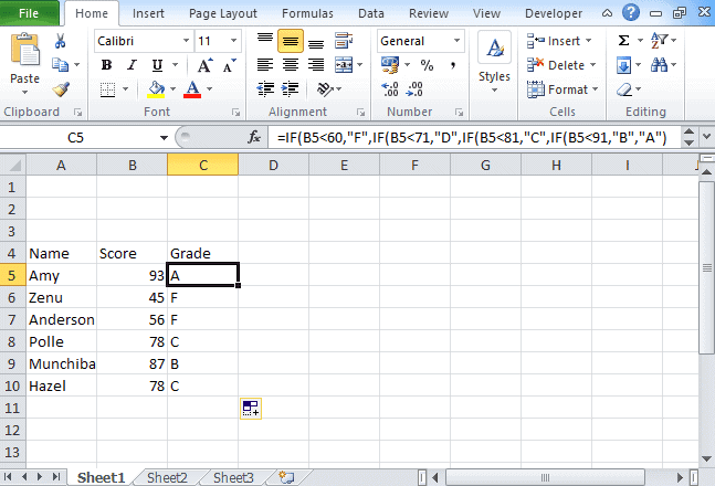
If the score is between 0 to 60, then Grade F
If the score is between 61 to 70, then Grade D
If the score is between 71 to 80, then Grade C
If the score is between 81 to 90, then Grade B
If the score is between 91 to 100, then Grade A

Then to test the condition the syntax of the formula becomes,

3) Excel If with Logical Test

There are 2 different types of conditions AND and OR. You can use the IF statement in excel between two values in both these conditions to perform the logical test.

AND Function: If you are performing the logical test based on AND function, then excel will give you TRUE as an outcome in every condition else it will return false.

OR Function: If you are using OR condition for the logical test, then excel will give you an outcome as TRUE if any of the situations match else it returns false.

For this, multiple testing is to be done using AND and OR function, you should gain expertise in using either or both of these with IF statement. Here we have used if the function with 3 conditions.

How to apply IF & AND function in Excel

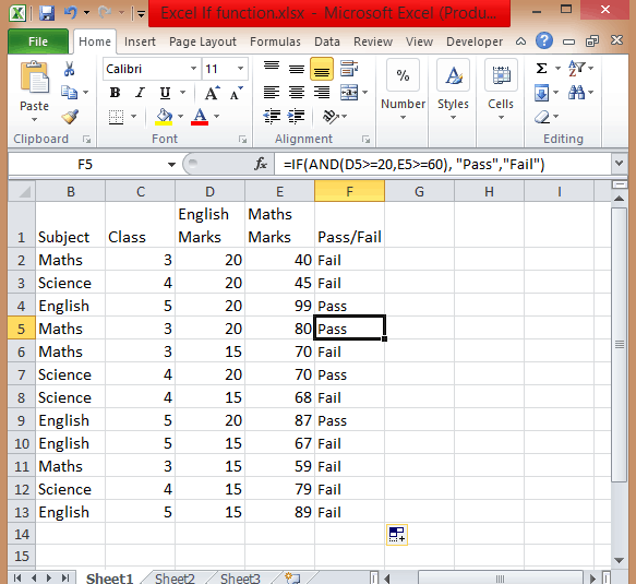
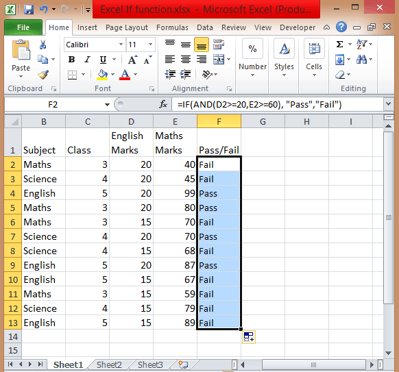
To perform this multiple if and statements in excel, we will take the data set for the student’s marks that contain fields such as English and Math’s Marks.
The score of the English subject is stored in the D column whereas the Maths score is stored in column E.
Let say a student passes the class if his or her score in English is greater than or equal to 20 and he or she scores more than 60 in Maths.
To create a report in matters of seconds, if formula combined with AND can suffice.
Type =IF( Excel will display the logical hint just below the cell F2. The parameters of this function are logical_test, value_if_true, value_if_false.
The first parameter contains the condition to be matched. You can use multiple If and AND conditions combined in this logical test.
In the second parameter, type the value that you want Excel to display if the condition is true. Similarly, in the third parameter type the value that will be displayed if your condition is false.

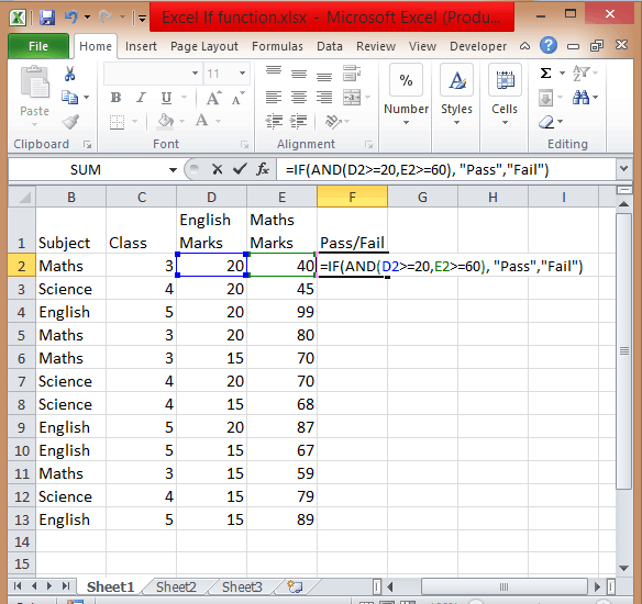
Apply If & And formula, you will get =IF(AND(D2>=20,E2>=60),”Pass”,”Fail”).

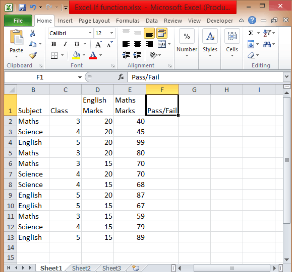
Add Pass/Fail column in the current table.

After you have applied this formula, you will find the result in the column.
Copy the formula from cell F2 and paste in all other cells from F3 to F13.

How to use If with Or function in Excel

To use If and Or statement excel, you need to apply a similar formula as you have applied for If & And with the only difference is that if any of the condition is true then it will show you True.

To apply the formula, you have to follow the above process. The formula is =IF((OR(D2>=20, E2>=60)), “Pass”, “Fail”). If the score is equal or greater than 20 for column D or the second score is equal or greater than 60 then the person is the pass.

How to Use If with And & Or function

If you want to test data based on several multiple conditions then you have to apply both And & Or functions at a single point in time. For example,

Situation 1: If column D>=20 and column E>=60

Situation 2: If column D>=15 and column E>=60

If any of the situations met, then the candidate is passed, else failed. The formula is

4) Excel If Statement with other functions

Above we have learned how to use excel if statement multiple conditions range with And/Or functions. Now we will be going to learn Excel If Statement with other excel functions.

Excel If with Sum, Average, Min, and Max functions

Let’s take an example where we want to calculate the performance of any student with Poor, Satisfactory, and Good.

If the data set has a predefined structure that will not allow any of the modifications. Then you can add values with this If formula:

Using the Sum function,

Using the Average function,

Using Max/Min,

If you want to find out the highest scores, using the Max function. You can also find the lowest scores using the Min function.

You can also find the lowest scores using the Min function.

If we combine both these formulas together, then we get

You can also call it as nested if functions with other excel functions. To get a result, you can use these if functions with various different functions that are used in excel.

So there are four different ways and types of excel if statements, that you can use according to the situation or condition. Start using it today.

So this is all about Excel If statement multiple conditions ranges, you can also check how to add bullets in excel in our next post.

I hope you found this tutorial useful

You may also like the following Excel tutorials:

Источник

VBA Named Range most efficient way to check if name exists

I have a routine, that fills a calendar with all important events for the commodity markets for each day of the following week. I have a calendar grid laid out on the page and have ten named cells for each day i.e. Monday1, Monday2 and so on (each day only goes up to 10 for now, i.e.Monday10), in each days column. BTW the cells are 2 cells wide and 2 cells deep. Many times there are more than 10 events for a given day. I am trying to test for the named range to see if it exists, if not copy the format of the last named range cell and name that cell the next name in the series.

I am only having two issues with the above, first and foremost is how to test to determine in a name for a named range already exists. I am currently iterating thru the entire list of ThisWorkbook.Names, which has thousands of named ranges in it. Since this iteration could be running over 100 times when the calendar is generating, it is wicked slow (as would be expected). Is there a better, faster way to check if a name already exists as a named range?

The second issue is how to copy the formatting of a 4 cell, merged cell, since the address always comes up as only the top left corner cell so offsetting the range doesn’t work appropriately. I hacked around to get this code to at least come up with the right range for the next merged cell group in the column

Recording a macro to drag the formatting down, shows this code.

Since Range(«G22:H23») is the same as cCell, and Range(«G22:H25») is the same as destRange. The following code should work, but doesn’t.

FYI, it doesn’t work if I select cCell and use Selection.AutoFill either.

Any thoughts on how to copy that cell formatting down the column one cell at a time when needed?

Update:

This now works for copying the formatting down from one merged cell to another of same size. For some reason setting destRange to the whole range (the copy cell and pastecell entire range as the macro recorder showed) didnt work but setting destRange to the cell range that needed formatting, and then doing a union of cCell and destRange worked, and made naming the new range easier.

Update #2

There is an issue with naming ranges in a For loop ( the code below is running inside a For loop). The first time the new rangeName is not found, Setting cCell to the prior range name and running through the code to copy the merged cell format and name the new range works fine. Here is the code

results in the following ranges

but if more than one new named range needs to be created the second time thru this code produces a range area as evidenced by the output shown below

so why does cCell’s address show as only the upper left cells address when run the first time, but the second time thru cCell’s address is shown as the whole merged cell range? And because it does, the next code line produces a range object error

Eliminating that code line and amending the first Set cCell to this;

produces the same error. I could kludge this by setting a counter, and if more than one, bypass that code line but that is not the preferred solution.

Источник

named range using an if statement with array formula for dependent dropdown

Stumped after looking for a bit.

I have a spreadsheet with items like so:

I want to create a dropdown based on Activity. I can do this in a typical cell (with ctrl + shift + enter for array formula):

But I can’t figure out how to put that formula into a named range properly. When I hit ctrl + shift + enter, no braces appear. When it’s without braces, it doesn’t seem to work, either (it shows the value as <. >).

Is there a way to make this work?

Thanks in advance

2 Answers 2

In the end, this wasn’t possible via a named range; I ended up doing a variant of dependent dropdowns with offsets as well as two pivots, based on the blog page from Darren’s comment above as well as this link. May be overkill, but at least I know how I got to it.

Setting up the first dropdown data source and data validation for the dropdown

For the first list, I created a pivot from the dropdown data source with row of column «Type» and values of count «Type» (the values aren’t that relevant, but I found it useful to just know how any elements to expect for later dependent items). This pivot is in the standard default pivot location on a new sheet, where the header row starts on A3. Using a pivot also sorts it by default alphabetically (which I wanted). Turn of all total columns.

I then created a named range («costCategory») with the following formula:

That basically makes a list of the items and removes any blanks. It’s not as dynamic as I’d like, but I think it’s very unlikely I’ll ever get beyond

100 items on the list so I decided to live with it.

I created another named range («emptyList») with the following formula:

So that I could also lock the first dropdown if the second, dependent one is selected (to prevent weird non-matching data issues).

For the table rows that needed the dropdowns, I put in the data validation for a list with this formula:

where $B3 is the second, dependent dropdown location.

Setting up the second, dependent dropdown data source and data validation 5. I created another pivot from the same data source, with rows of «Type» and «Desc», and values of count of «Type» (again, the values not a big deal). The pivot layout was set to tabular, repeating labels, no totals or subtotals. I put this pivot next to the other one, with the first header row starting at E3. It also alpha sorts.

I put in helper columns to determine where the list starts for a particular parent of the dependent dropdown, and the number of rows of that list. It uses the same arbitrary long ranges approach as in the first dropdown — just put in a number of rows unlikely to be exceeded in the pivot. In col C, for getting the first row where the dependent data starts, I put this formula:

In col D, for getting the number of cols where there is dependent data, I put this formula:

Finally, in the column with the dependent dropdown (col B), I used the following data validation rule:

Which basically takes the range that’s found in the helper cols to make the dropdown list.

When these formulas are extended, they increment (A3 to A4, B3 to B4, etc.) so that they all still work even as you add rows to the listobject table.

Источник

How to Create Named Ranges in Excel (A Step-by-step Guide)

What’s in the name?

If you are working with Excel spreadsheets, it could mean a lot of time saving and efficiency.

In this tutorial, you’ll learn how to create Named Ranges in Excel and how to use it to save time.

This Tutorial Covers:

Named Ranges in Excel – An Introduction

If someone has to call me or refer to me, they will use my name (instead of saying a male is staying in so and so place with so and so height and weight).

Similarly, in Excel, you can give a name to a cell or a range of cells.

Now, instead of using the cell reference (such as A1 or A1:A10), you can simply use the name that you assigned to it.

For example, suppose you have a data set as shown below:

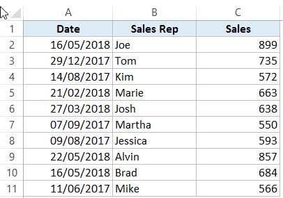
In this data set, if you have to refer to the range that has the Date, you will have to use A2:A11 in formulas. Similarly, for Sales Rep and Sales, you will have to use B2:B11 and C2:C11.

While it’s alright when you only have a couple of data points, but in case you huge complex data sets, using cell references to refer to data could be time-consuming.

Excel Named Ranges makes it easy to refer to data sets in Excel.

You can create a named range in Excel for each data category, and then use that name instead of the cell references. For example, dates can be named ‘Date’, Sales Rep data can be named ‘SalesRep’ and sales data can be named ‘Sales’.

You can also create a name for a single cell. For example, if you have the sales commission percentage in a cell, you can name that cell as ‘Commission’.

Benefits of Creating Named Ranges in Excel

Here are the benefits of using named ranges in Excel.

Use Names instead of Cell References

When you create Named Ranges in Excel, you can use these names instead of the cell references.

For example, you can use =SUM(SALES) instead of =SUM(C2:C11) for the above data set.

Have a look at ṭhe formulas listed below. Instead of using cell references, I have used the Named Ranges.

Number of sales with value more than 500: =COUNTIF(Sales,”>500″)
Sum of all the sales done by Tom: =SUMIF(SalesRep,”Tom”,Sales)
Commission earned by Joe (sales by Joe multiplied by commission percentage):
=SUMIF(SalesRep,”Joe”,Sales)*Commission

You would agree that these formulas are easy to create and easy to understand (especially when you share it with someone else or revisit it yourself.

No Need to Go Back to the Dataset to Select Cells

Another significant benefit of using Named Ranges in Excel is that you don’t need to go back and select the cell ranges.

You can just type a couple of alphabets of that named range and Excel will show the matching named ranges (as shown below):

Named Ranges Make Formulas Dynamic

By using Named Ranges in Excel, you can make Excel formulas dynamic.

For example, in the case of sales commission, instead of using the value 2.5%, you can use the Named Range.

Now, if your company later decides to increase the commission to 3%, you can simply update the Named Range, and all the calculation would automatically update to reflect the new commission.

How to Create Named Ranges in Excel

Here are three ways to create Named Ranges in Excel:

Method #1 – Using Define Name

Here are the steps to create Named Ranges in Excel using Define Name:

This will create a Named Range SALESREP.

Method #2: Using the Name Box

Select the range for which you want to create a name (do not select headers).
Go to the Name Box on the left of Formula bar and Type the name of the with which you want to create the Named Range.
Note that the Name created here will be available for the entire Workbook. If you wish to restrict it to a worksheet, use Method 1.

Method #3: Using Create From Selection Option

This is the recommended way when you have data in tabular form, and you want to create named range for each column/row.

For example, in the dataset below, if you want to quickly create three named ranges (Date, Sales_Rep, and Sales), then you can use the method shown below.

Here are the steps to quickly create named ranges from a dataset:

This will create three Named Ranges – Date, Sales_Rep, and Sales.

Note that it automatically picks up names from the headers. If there are any space between words, it inserts an underscore (as you can’t have spaces in named ranges).

Naming Convention for Named Ranges in Excel

There are certain naming rules you need to know while creating Named Ranges in Excel:

The first character of a Named Range should be a letter and underscore character(_), or a backslash(). If it’s anything else, it will show an error. The remaining characters can be letters, numbers, special characters, period, or underscore.
You can not use names that also represent cell references in Excel. For example, you can’t use AB1 as it is also a cell reference.
You can’t use spaces while creating named ranges. For example, you can’t have Sales Rep as a named range. If you want to combine two words and create a Named Range, use an underscore, period or uppercase characters to create it. For example, you can have Sales_Rep, SalesRep, or SalesRep.
- While creating named ranges, Excel treats uppercase and lowercase the same way. For example, if you create a named range SALES, then you will not be able to create another named range such as ‘sales’ or ‘Sales’.
A Named Range can be up to 255 characters long.

Too Many Named Ranges in Excel? Don’t Worry

Sometimes in large data sets and complex models, you may end up creating a lot of Named Ranges in Excel.

What if you don’t remember the name of the Named Range you created?

Don’t worry – here are some useful tips.

Getting the Names of All the Named Ranges

Here are the steps to get a list of all the named ranges you created:

This will give you a list of all the Named Ranges in that workbook. To use a named range (in formulas or a cell), double click on it.

Displaying the Matching Named Ranges

If you have some idea about the Name, type a few initial characters, and Excel will show a drop down of the matching names.

How to Edit Named Ranges in Excel

If you have already created a Named Range, you can edit it using the following steps:

Useful Named Range Shortcuts (the Power of F3)

Here are some useful keyboard shortcuts that will come handy when you are working with Named Ranges in Excel:

To get a list of all the Named Ranges and pasting it in Formula: F3
To create new name using Name Manager Dialogue Box: Control + F3
To create Named Ranges from Selection: Control + Shift + F3

Creating Dynamic Named Ranges in Excel

So far in this tutorial, we have created static Named Ranges.

This means that these Named Ranges would always refer to the same dataset.

For example, if A1:A10 has been named as ‘Sales’, it would always refer to A1:A10.

If you add more sales data, then you would have to manually go and update the reference in the named range.

In the world of ever-expanding data sets, this may end up taking up a lot of your time. Every time you get new data, you may have to update the Named Ranges in Excel.

To tackle this issue, we can create Dynamic Named Ranges in Excel that would automatically account for additional data and include it in the existing Named Range.

For example, For example, if I add two additional sales data points, a dynamic named range would automatically refer to A1:A12.

This kind of Dynamic Named Range can be created by using Excel INDEX function. Instead of specifying the cell references while creating the Named Range, we specify the formula. The formula automatically updated when the data is added or deleted.

Let’s see how to create Dynamic Named Ranges in Excel.

Suppose we have the sales data in cell A2:A11.

Here are the steps to create Dynamic Named Ranges in Excel:

1. Go to the Formula tab and click on Define Name.
2. In the New Name dialogue box type the following:
  - Name: Sales
  - Scope: Workbook
  - Refers to: =$A$2:INDEX($A$2:$A$100,COUNTIF($A$2:$A$100,”<>”&””))
3. Click OK.

You now have a dynamic named range with the name ‘Sales’. This would automatically update whenever you add data to it or remove data from it.

How does Dynamic Named Ranges Work?

To explain how this work, you need to know a bit more about Excel INDEX function.

Most people use INDEX to return a value from a list based on the row and column number.

But the INDEX function also has another side to it.

It can be used to return a cell reference when it is used as a part of a cell reference.

For example, here is the formula that we have used to create a dynamic named range:

INDEX($A$2:$A$100,COUNTIF($A$2:$A$100,”<>”&””) –> This part of the formula is expected to return a value (which would be the 10th value from the list, considering there are ten items).

However, when used in front of a reference (= $A$2: INDEX($A$2:$A$100,COUNTIF($A$2:$A$100,”<>”&””)) ) it returns the reference to the cell instead of the value.

Hence, here it returns =$A$2:$A$11

If we add two additional values to the sales column, it would then return =$A$2:$A$13

When you add new data to the list, Excel COUNTIF function returns the number of non-blank cells in the data. This number is used by the INDEX function to fetch the cell reference of the last item in the list.

Note:

This would only work if there are no blank cells in the data.
In the example taken above, I have assigned a large number of cells (A2:A100) for the Named Range formula. You can adjust this based on your data set.

You can also use OFFSET function to create a Dynamic Named Ranges in Excel, however, since OFFSET function is volatile, it may lead a slow Excel workbook. INDEX, on the other hand, is semi-volatile, which makes it a better choice to create Dynamic Named Ranges in Excel.

You may also like the following Excel resources:

Источник

I’m trying to write a formula that will populate a cell based on the information in another cell.

Stated one way: «If the value in cell A2 equals the name of any of the people in this named range, then set the value in this cell to «SME», but if the value in cell A2 equals the name of anyone in this other named range, then set the value in this cell to «L3», etc.

Stated another way:

If the value in [cell] is [any of the values in SME named range], then «SME»; If the value in [cell] is [any of the values in the L3_ named range], then «L3»; If the value in [cell] is [any of the values in the L2_ named range], then «L2»

SME, L3_ and L2_ are all named ranges that include the names of people.

I haven’t been able to get a legitimate value from any of my attempts, so either I’m missing something (most likely) or what I’m trying to do can’t be done. I’m trying to avoid a lengthy formula that has multiple «OR» statements embedded because at least one of the named ranges has 20 values in it.

If you have questions on this, if what I’m asking isn’t clear, let me know. I appreciate any help.

Thanks,
Cherie

Источник

Let me try this again, I’ve been searching the web and can’t seem to find anything. What i’m trying to do is in excel have a bunc of named range list conditional based on a value of another cell. The problem I’m running into character limit when I setup the data validation and put all my IF statements in source textbox. If i just put two conditions it seems to work fine, but that won’t work for me. Here is my example data, based on the B column value I want to display the valid sub-items for it. Like I mentioned I have 20 or so different possible values that could be in column B.

          B     C
      1 ENG     dropdown of all engineering sub-categories
      2 PRO     dropdown of all production sub-categories
      3 PER     ...
      4 PAY
      5 ENG     dropdown of all engineering sub-categories  
      6 ENG     dropdown of all engineering sub-categories

When i try to setup my data validation list on column C1, I put in the following…

=IF($E$5="CAR", CA,
IF($E$5="DCC", DCC,
IF($E$5="ENG", ENG,
IF$E$5="ENV", ENV,
IF$E$5="FBI", BI,
IF$E$5="FGL", GL, 
IF$E$5="FAP", AP, 
IF$E$5="FRE", AR, 
IF$E$5="FTX", Tax, 
IF$E$5="ORM", OAR, 
IF$E$5="PAY", PAY, 
IF$E$5="PIR", PER, 
IF$E$5="PRO", PRO, 
IF$E$5="PUR", PUR, 
IF$E$5="RSK", RM, 
IF$E$5="SLM", Sales,
IF$E$5="WFS", WAR)))))))))))))))))

I’m only able to type in maybe half of my IF condition. I tried VLOOKUP but that only allows for 1 value to be put in column C, and I want it to be a dropdown. Any help would be much apprecriated.

Источник

To perform complicated and powerful data analysis, you need to test various conditions at a single point in time. The data analysis might require logical tests also within these multiple conditions.

For this, you need to perform Excel if statement with multiple conditions or ranges that include various If functions in a single formula.

1) Excel If Statement

If you want to test a condition to get two outcomes then you can use this Excel If statement.

=If(Marks>=40, “Pass”)

2) Nested If Statement

Let’s take an example that met the below-mentioned condition

If the score is between 0 to 60, then Grade F
If the score is between 61 to 70, then Grade D
If the score is between 71 to 80, then Grade C
If the score is between 81 to 90, then Grade B
If the score is between 91 to 100, then Grade A

Then to test the condition the syntax of the formula becomes,

=If(B5<60, “F”,If(B5<71, “D”, If(B5<81,”C”,If(B5<91,”B”,”A”)

3) Excel If with Logical Test

There are 2 different types of conditions AND and OR. You can use the IF statement in excel between two values in both these conditions to perform the logical test.

AND Function: If you are performing the logical test based on AND function, then excel will give you TRUE as an outcome in every condition else it will return false.

OR Function: If you are using OR condition for the logical test, then excel will give you an outcome as TRUE if any of the situations match else it returns false.

For this, multiple testing is to be done using AND and OR function, you should gain expertise in using either or both of these with IF statement. Here we have used if the function with 3 conditions.

How to apply IF & AND function in Excel

To perform this multiple if and statements in excel, we will take the data set for the student’s marks that contain fields such as English and Math’s Marks.
The score of the English subject is stored in the D column whereas the Maths score is stored in column E.
Let say a student passes the class if his or her score in English is greater than or equal to 20 and he or she scores more than 60 in Maths.
To create a report in matters of seconds, if formula combined with AND can suffice.
Type =IF( Excel will display the logical hint just below the cell F2. The parameters of this function are logical_test, value_if_true, value_if_false.
The first parameter contains the condition to be matched. You can use multiple If and AND conditions combined in this logical test.
In the second parameter, type the value that you want Excel to display if the condition is true. Similarly, in the third parameter type the value that will be displayed if your condition is false.

Apply If & And formula, you will get =IF(AND(D2>=20,E2>=60),”Pass”,”Fail”).

Add Pass/Fail column in the current table.

After you have applied this formula, you will find the result in the column.
Copy the formula from cell F2 and paste in all other cells from F3 to F13.

How to use If with Or function in Excel

To use If and Or statement excel, you need to apply a similar formula as you have applied for If & And with the only difference is that if any of the condition is true then it will show you True.

How to Use If with And & Or function

If you want to test data based on several multiple conditions then you have to apply both And & Or functions at a single point in time. For example,

Situation 1: If column D>=20 and column E>=60

Situation 2: If column D>=15 and column E>=60

If any of the situations met, then the candidate is passed, else failed. The formula is

=IF(OR(AND(D2>=20, E2>=60), AND(D2>=20, E2>=60)), “Pass”, “Fail”).

4) Excel If Statement with other functions

Above we have learned how to use excel if statement multiple conditions range with And/Or functions. Now we will be going to learn Excel If Statement with other excel functions.

Excel If with Sum, Average, Min, and Max functions

Let’s take an example where we want to calculate the performance of any student with Poor, Satisfactory, and Good.

If the data set has a predefined structure that will not allow any of the modifications. Then you can add values with this If formula:

=If((A2+B2)>=50, “Good”, If((A2+B2)=>30, “Satisfactory”, “Poor”))

Using the Sum function,

=If(Sum(A2:B2)>=120, “Good”, If(Sum(A2:B2)>=100, “Satisfactory”, “Poor”))

Using the Average function,

=If(Average(A2:B2)>=40, “Good”, If(Average(A2:B2)>=25, “Satisfactory”, “Poor”))

Using Max/Min,

If you want to find out the highest scores, using the Max function. You can also find the lowest scores using the Min function.

=If(C2=Max($C$2:$C$10), “Best result”, “ “)

You can also find the lowest scores using the Min function.

=If(C2=Min($C$2:$C$10), “Worst result”, “ “)

If we combine both these formulas together, then we get

=If(C2=Max($C$2:$C$10), “Best result”, If(C2=Min($C$2:$C$10), “Worst result”, “ “))

You can also call it as nested if functions with other excel functions. To get a result, you can use these if functions with various different functions that are used in excel.

So there are four different ways and types of excel if statements, that you can use according to the situation or condition. Start using it today.

So this is all about Excel If statement multiple conditions ranges, you can also check how to add bullets in excel in our next post.

I hope you found this tutorial useful

You may also like the following Excel tutorials:

Multiple If Statements in Excel
Excel Logical test
How to Compare Two Columns in Excel (using VLOOKUP & IF)
Using IF Function with Dates in Excel (Easy Examples)

Источник

Many people usually asked that how to write an excel nested if statements based on multiple ranges of cells to return different values in a cell? How to nested if statement using date ranges? How to use nested if statement between different values in excel 2013 or 2016?

Nested IF statements based on multiple ranges
Nested IF Statement Using Date Ranges
Nested IF Statements For A Range Of Cells
Nested IF Statement between different values

This post will guide you how to understand excel nested if statements through some classic examples.

Table of Contents

Nested IF statements based on multiple ranges
Nested IF Statement Using Date Ranges
Nested IF Statements For A Range Of Cells
Nested IF Statement between different values
- Related Functions

Nested IF statements based on multiple ranges

Assuming that you want to reflect the below request through nested if statements:

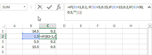
a) If 1<B1<0, Then return 0.1

b) If 0.99<B1<5, then return 0.15

c) If 4.99<B1<15, then return 0.2

d) If 14.99<B1<30, then return 0.5

So if B1 cell was “14.5”, then the formula should be returned “0.2” in the cell.

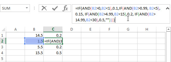
From above logic request, we can get that it need 4 if statements in the excel formula, and there are multiple ranges so that we can combine with logical function AND in the nested if statements. The below is the nested if statements that I have tested.

=IF(AND(B1>0,B1<1),0.1,IF(AND(B1>0.99, B1<5),0.15, IF(AND(B1>4.99,B1<15),0.2, IF(AND(B1>14.99,B1<30),0.5,””))))

If you don’t want to use AND function in the above nested if statement, can try the below formula:

=IF(B1<1,0.1, If(B1<5,0.15,IF(B1<15,0.2,IF(B1<30,0.5,””))))

Nested IF Statement Using Date Ranges

I want to write a nested IF statement to calculated the right Quarter based one the criteria in the below table.

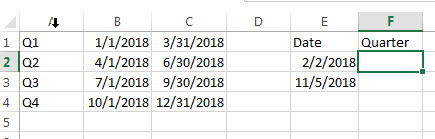
According to the request, we need to compare date ranges, such as: if B1<E2<C1, then return A1.

So we can consider to use AND logical function in the nested if statement. The formula is as follows:

=IF(AND(E2>B1,E2<C1),A1,IF(AND(E2>B2,E2<C2),A2,IF(AND(E2>B3,E2<C3),A3,IF(AND(E2>B4,E2<C3),A4))))

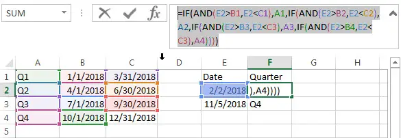
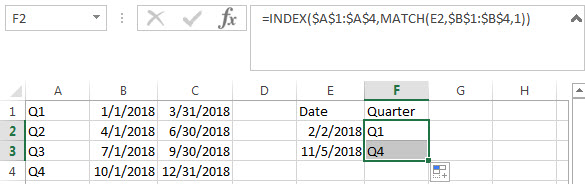
Or we can use INDEX function and combine with MATCH Function to get the right quarter.

=INDEX($A$1:$A$4,MATCH(E2,$B$1:$B$4,1))

Nested IF Statements For A Range Of Cells

If you have the following requirement and need to write a nested IF statement in excel:

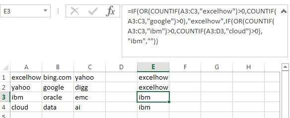
If any of the cells A1 to C1 contain “excelhow”, then return “excelhow” in the cell E1.

If any of the cells A1 to C1 contain “google”, then return “excelhow” in the cell E1.

If any of the cells A1 to C1 contain “ibm”, then return “ibm” in the cell E1.

If any of the cells A1 to C1 contain “Cloud”, then return “ibm” in the cell E1.

How to check if cell ranges A1:C1 contain another string, using “COUNTIF” function is a good choice.

Countif function: Counts the number of cells within a range that meet the given criteria

Let’s try to test the below nested if statement:

=IF(OR(COUNTIF(A3:C3,"excelhow")>0,COUNTIF(A3:C3,"google")>0),"excelhow",IF(OR(COUNTIF(A3:C3,"ibm")>0,COUNTIF(A3:D3,"cloud")>0),"ibm",""))

Nested IF Statement between different values

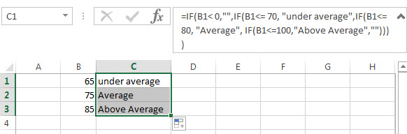
Assuming you have the following different range values, if the B1 has the value 65, then expected to return “under average”in cell C1, if the Cell B1 has the value 75, then return “average” in cell C1. And if the Cell B1 has the value 85, then return “above average” in the cell C1.

0-70	under average
71-80	average
81-100	above average

How do I format the nested if statement in Cell C1 to display the right value? Just try to use the below nested if function or using INDEX function.

=IF(B1< 0,"",IF(B1<= 70, "under average",IF(B1<=80, "Average", IF(B1<=100,"Above Average",""))))

Excel IF function
The Excel IF function perform a logical test to return one value if the condition is TRUE and return another value if the condition is FALSE. The IF function is a build-in function in Microsoft Excel and it is categorized as a Logical Function.The syntax of the IF function is as below:= IF (condition, [true_value], [false_value])….
Excel nested if function
The nested IF function is formed by multiple if statements within one Excel if function. This excel nested if statement makes it possible for a single formula to take multiple actions…
Excel AND function
The Excel AND function returns TRUE if all of arguments are TRUE, and it returns FALSE if any of arguments are FALSE.The syntax of the AND function is as below:= AND (condition1,[condition2],…) …
Excel COUNTIF function
The Excel COUNTIF function will count the number of cells in a range that meet a given criteria.This function can be used to count the different kinds of cells with number, date, text values, blank, non-blanks, or containing specific characters.etc.The syntax of the COUNTIF function is as below:= COUNTIF (range, criteria) …
Excel INDEX function
The Excel INDEX function returns a value from a table based on the index (row number and column number)The INDEX function is a build-in function in Microsoft Excel and it is categorized as a Lookup and Reference Function.The syntax of the INDEX function is as below:= INDEX (array, row_num,[column_num])…
Excel MATCH function
The Excel MATCH function search a value in an array and returns the position of that item.The MATCH function is a build-in function in Microsoft Excel and it is categorized as a Lookup and Reference Function.The syntax of the MATCH function is as below:= MATCH (lookup_value, lookup_array, [match_type])….

Источник

What’s in the name?

If you are working with Excel spreadsheets, it could mean a lot of time saving and efficiency.

In this tutorial, you’ll learn how to create Named Ranges in Excel and how to use it to save time.

Named Ranges in Excel – An Introduction
Benefits of Creating Named Ranges in Excel
- Use Names instead of Cell References
- No Need to Go Back to the Dataset to Select Cells
- Named Ranges Make Formulas Dynamic
How to Create Named Ranges in Excel
- Method #1 – Using Define Name
- Method #2: Using the Name Box
- Method #3: Using Create From Selection Option
- Naming Convention for Named Ranges in Excel
Too Many Named Ranges in Excel? Don’t Worry
- Getting the Names of All the Named Ranges
- Displaying the Matching Named Ranges
How to Edit Named Ranges in Excel
Useful Named Range Shortcuts (the Power of F3)
Creating Dynamic Named Ranges in Excel
- How does Dynamic Named Ranges Work?

Named Ranges in Excel – An Introduction

If someone has to call me or refer to me, they will use my name (instead of saying a male is staying in so and so place with so and so height and weight).

Right?

Similarly, in Excel, you can give a name to a cell or a range of cells.

Now, instead of using the cell reference (such as A1 or A1:A10), you can simply use the name that you assigned to it.

For example, suppose you have a data set as shown below:

In this data set, if you have to refer to the range that has the Date, you will have to use A2:A11 in formulas. Similarly, for Sales Rep and Sales, you will have to use B2:B11 and C2:C11.

While it’s alright when you only have a couple of data points, but in case you huge complex data sets, using cell references to refer to data could be time-consuming.

Excel Named Ranges makes it easy to refer to data sets in Excel.

You can also create a name for a single cell. For example, if you have the sales commission percentage in a cell, you can name that cell as ‘Commission’.

Benefits of Creating Named Ranges in Excel

Here are the benefits of using named ranges in Excel.

Use Names instead of Cell References

When you create Named Ranges in Excel, you can use these names instead of the cell references.

For example, you can use =SUM(SALES) instead of =SUM(C2:C11) for the above data set.

Have a look at ṭhe formulas listed below. Instead of using cell references, I have used the Named Ranges.

Number of sales with value more than 500: =COUNTIF(Sales,”>500″)
Sum of all the sales done by Tom: =SUMIF(SalesRep,”Tom”,Sales)
Commission earned by Joe (sales by Joe multiplied by commission percentage):
=SUMIF(SalesRep,”Joe”,Sales)*Commission

You would agree that these formulas are easy to create and easy to understand (especially when you share it with someone else or revisit it yourself.

No Need to Go Back to the Dataset to Select Cells

Another significant benefit of using Named Ranges in Excel is that you don’t need to go back and select the cell ranges.

You can just type a couple of alphabets of that named range and Excel will show the matching named ranges (as shown below):

Named Ranges Make Formulas Dynamic

By using Named Ranges in Excel, you can make Excel formulas dynamic.

For example, in the case of sales commission, instead of using the value 2.5%, you can use the Named Range.

Now, if your company later decides to increase the commission to 3%, you can simply update the Named Range, and all the calculation would automatically update to reflect the new commission.

How to Create Named Ranges in Excel

Here are three ways to create Named Ranges in Excel:

Method #1 – Using Define Name

Here are the steps to create Named Ranges in Excel using Define Name:

This will create a Named Range SALESREP.

Method #2: Using the Name Box

Select the range for which you want to create a name (do not select headers).
Go to the Name Box on the left of Formula bar and Type the name of the with which you want to create the Named Range.
Note that the Name created here will be available for the entire Workbook. If you wish to restrict it to a worksheet, use Method 1.

Method #3: Using Create From Selection Option

This is the recommended way when you have data in tabular form, and you want to create named range for each column/row.

For example, in the dataset below, if you want to quickly create three named ranges (Date, Sales_Rep, and Sales), then you can use the method shown below.

Here are the steps to quickly create named ranges from a dataset:

This will create three Named Ranges – Date, Sales_Rep, and Sales.

Note that it automatically picks up names from the headers. If there are any space between words, it inserts an underscore (as you can’t have spaces in named ranges).

Naming Convention for Named Ranges in Excel

There are certain naming rules you need to know while creating Named Ranges in Excel:

The first character of a Named Range should be a letter and underscore character(_), or a backslash(). If it’s anything else, it will show an error. The remaining characters can be letters, numbers, special characters, period, or underscore.
You can not use names that also represent cell references in Excel. For example, you can’t use AB1 as it is also a cell reference.
You can’t use spaces while creating named ranges. For example, you can’t have Sales Rep as a named range. If you want to combine two words and create a Named Range, use an underscore, period or uppercase characters to create it. For example, you can have Sales_Rep, SalesRep, or SalesRep.
- While creating named ranges, Excel treats uppercase and lowercase the same way. For example, if you create a named range SALES, then you will not be able to create another named range such as ‘sales’ or ‘Sales’.
A Named Range can be up to 255 characters long.

Too Many Named Ranges in Excel? Don’t Worry

Sometimes in large data sets and complex models, you may end up creating a lot of Named Ranges in Excel.

What if you don’t remember the name of the Named Range you created?

Don’t worry – here are some useful tips.

Getting the Names of All the Named Ranges

Here are the steps to get a list of all the named ranges you created:

This will give you a list of all the Named Ranges in that workbook. To use a named range (in formulas or a cell), double click on it.

Displaying the Matching Named Ranges

If you have some idea about the Name, type a few initial characters, and Excel will show a drop down of the matching names.

How to Edit Named Ranges in Excel

If you have already created a Named Range, you can edit it using the following steps:

Useful Named Range Shortcuts (the Power of F3)

Here are some useful keyboard shortcuts that will come handy when you are working with Named Ranges in Excel:

To get a list of all the Named Ranges and pasting it in Formula: F3
To create new name using Name Manager Dialogue Box: Control + F3
To create Named Ranges from Selection: Control + Shift + F3

Creating Dynamic Named Ranges in Excel

So far in this tutorial, we have created static Named Ranges.

This means that these Named Ranges would always refer to the same dataset.

For example, if A1:A10 has been named as ‘Sales’, it would always refer to A1:A10.

If you add more sales data, then you would have to manually go and update the reference in the named range.

In the world of ever-expanding data sets, this may end up taking up a lot of your time. Every time you get new data, you may have to update the Named Ranges in Excel.

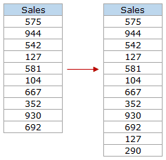
To tackle this issue, we can create Dynamic Named Ranges in Excel that would automatically account for additional data and include it in the existing Named Range.

For example, For example, if I add two additional sales data points, a dynamic named range would automatically refer to A1:A12.

Let’s see how to create Dynamic Named Ranges in Excel.

Suppose we have the sales data in cell A2:A11.

Here are the steps to create Dynamic Named Ranges in Excel:

1. Go to the Formula tab and click on Define Name.
2. In the New Name dialogue box type the following:
  - Name: Sales
  - Scope: Workbook
  - Refers to: =$A$2:INDEX($A$2:$A$100,COUNTIF($A$2:$A$100,”<>”&””))
3. Click OK.

Done!

You now have a dynamic named range with the name ‘Sales’. This would automatically update whenever you add data to it or remove data from it.

How does Dynamic Named Ranges Work?

To explain how this work, you need to know a bit more about Excel INDEX function.

Most people use INDEX to return a value from a list based on the row and column number.

But the INDEX function also has another side to it.

It can be used to return a cell reference when it is used as a part of a cell reference.

For example, here is the formula that we have used to create a dynamic named range:

=$A$2:INDEX($A$2:$A$100,COUNTIF($A$2:$A$100,"<>"&""))

INDEX($A$2:$A$100,COUNTIF($A$2:$A$100,”<>”&””) –> This part of the formula is expected to return a value (which would be the 10th value from the list, considering there are ten items).

However, when used in front of a reference (=$A$2:INDEX($A$2:$A$100,COUNTIF($A$2:$A$100,”<>”&””))) it returns the reference to the cell instead of the value.

Hence, here it returns =$A$2:$A$11

If we add two additional values to the sales column, it would then return =$A$2:$A$13

Note:

This would only work if there are no blank cells in the data.
In the example taken above, I have assigned a large number of cells (A2:A100) for the Named Range formula. You can adjust this based on your data set.

You may also like the following Excel resources:

Free Excel Templates.
Free Online Excel Training (7-Part Online Video Course).
Useful Excel Macro Code Examples.
10 Advanced Excel VLOOKUP Examples.
Creating a Drop Down List in Excel.
Creating a Named Range in Google Sheets.
How to Reference Another Sheet or Workbook in Excel
How to Delete Named Range in Excel?

Источник

Remove From My Forums

Question
While working on an excel 2003 add-in with vb.net, I need to check if a name range exists in the workbook.

Currently I have to loop through all the names and do a comparison like the following code. This becomes very slow when a workbook has over 6000 name ranges.

For
Each nm
As Excel.Name
In activeWorkbook.Names

If nm.Name.equals(«mysearch»)
Then

do something

End
If

Next nm

I am wondering if there is a better way to do that. Something like Hashtable.ContainsKey() would be nice. Or something like a SQL select where clause because all my names starts with «Period_»

Thanks

I also tried use a try-catch solution, assuming it exists and catch the exception if it doesn’t, like the following code, it is also not ideal.

Try

Dim namedRange As Name = activeWorkbook.Names.Item(strName)

Return True

Catch

Return False

End Try

Answers

I haven’t try this is VB.NET but have done it in Excel VBA. You can use the evaluate function to determine if the named range exists.

ValueExist = evaluate(«mysearch»)

Thjis will return the error string «Error 2029» if the value doesn’t exist and return the data from the first cell if the string does exist. the only problem is if the first cell contains the string «Error 2029».

The evaluate function acts exactly like a worksheet function except you call it from VBA without using the equal sign. for example

=Sum(A1:A20) is the same as Evaluate(«SUM(A1:A20)»)

jdweng
- Marked as answer by
  
  Tuesday, October 26, 2010 12:21 PM

Источник

TLDR; seems like CF thinks my formula with named range is an array, and I want it to function like a flat formula.

Long time lurker, first time poster!

I have been creating nice elaborate conditional formatting formulas for a while now. However, I have always had a challenge when using these with named ranges. The formulas work great when in a cell, but when placed into CF, they fail.

Perhaps my issue is related to the way in which CF seems to already identify these formulas as arrays. Perhaps somebody can help me understand how best to overcome this issue. I’ll link a document for illustration.

So when I place escalating numbers in A1:J1, and place in A2:J2 this formula

=IF(TheNums>4,TRUE,FALSE)

then E2:J2 all come back TRUE. Placing the same formula into CF comes back all FALSE. If I enter the same formula as an array with CSE, I get FALSE all across.

Can somebody help with my syntax to hopefully stop this from failing?

Thanks so much!
Kyle

[linked here]

Источник

This tutorial demonstrates how to use the IF Function in Excel and Google Sheets to create If Then Statements.

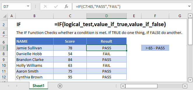
IF Function Overview

The IF Function Checks whether a condition is met. If TRUE do one thing, if FALSE do another.

How to Use the IF Function

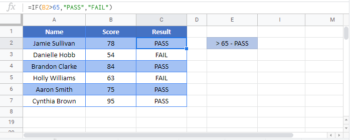
Here’s a very basic example so you can see what I mean. Try typing the following into Excel:

=IF( 2 + 2 = 4,"It’s true", "It’s false!")

Since 2 + 2 does in fact equal 4, Excel will return “It’s true!”. If we used this:

=IF( 2 + 2 = 5,"It’s true", "It’s false!")

Now Excel will return “It’s false!”, because 2 + 2 does not equal 5.

Here’s how you might use the IF statement in a spreadsheet.

=IF(C4-D4>0,C4-D4,0)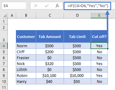

You run a sports bar and you set individual tab limits for different customers. You’ve set up this spreadsheet to check if each customer is over their limit, in which case you’ll cut them off until they pay their tab.

You check if C4-D4 (their current tab amount minus their limit), is greater than 0. This is your logical test. If this is true, IF returns “Yes” – you should cut them off. If this is false, IF returns “No” – you let them keep drinking.

What can IF Return?

Above we returned a text string, “Yes” or “No”. But you can also return numbers, or even other formulas.

Let’s say some of your customers are running up big tabs. To discourage this, you’re going to start charging interest on customers who go over their limit.

You can use IF for that:

=IF(C4>D4,C4*0.03,0)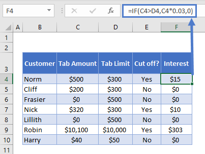

If the tab is higher than the limit, return the tab multiplied by 0.03, which returns 3% of the tab. Otherwise, return 0: they aren’t over their tab, so you won’t charge interest.

Using IF with AND

You can combine IF with Excel’s AND Function to test more than one condition. Excel will only return TRUE if ALL of the tests are true.

So, you implemented your interest rate. But some of your regulars are complaining. They’ve always paid their tabs in the past, why are you cracking down on them now? You come up with a solution: you won’t charge interest to certain trusted customers.

You make a new column to your spreadsheet to identify trusted customers, and update your IF statement with an AND function:

=IF(AND(C4>D4, F4="No"),C4*0.03,0)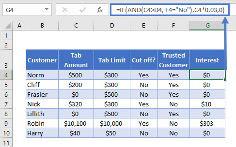

IF AND

Let’s look at the AND part separately:

AND(C4>D4, F4="No")

Note the two conditions:

C4>D4: checking if they’re over their tab limit, as before
F4=”No”: this is the new bit, checking if they are not a trusted customer

So now we only return the interest rate if the customer is over their tab, AND we have “No” in the trusted customer column. Your regulars are happy again.

Using IF with OR

The OR Function allows you to test more than one condition, returning TRUE if any conditions are met.

Maybe customers being over their tab is not the only reason you’d cut them off. Maybe you give some people a temporary ban for other reasons, gambling on the premises perhaps.

So you add a new column to identify banned customers, and update your “Cut off?” column with an OR test:

=IF(OR(C4>D4,E4="Yes"),"Yes","No")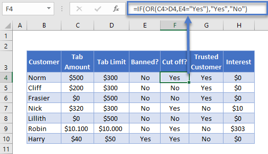

Looking just at the OR part:

OR(C4>D4,E4="Yes")

There are two conditions:

C4>D4: checking if they’re over their tab limit
F4=”Yes”: the new part, checking if they are currently banned

This will evaluate to true if they are over their tab, or if there is a “Yes” in column E. As you can see, Harry is cut off now, even though he’s not over his tab limit.

Using IF with XOR

The XOR Function returns TRUE if only one condition is met. If more than one condition is met (or not conditions are met). It returns FALSE.

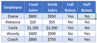
An example might make this clearer. Imagine you want to start giving monthly bonuses to your staff :

If they sell over $800 in food, or over $800 in drinks, you’ll give them a half bonus
If they sell over $800 in both, you’ll give them a full bonus
If they sell under $800 in both, they don’t get any bonus.

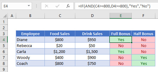
You already know how to work out if they get the full bonus. You’d just use IF with AND, as described earlier.

=IF(AND(C4>800,D4>800),"Yes","No")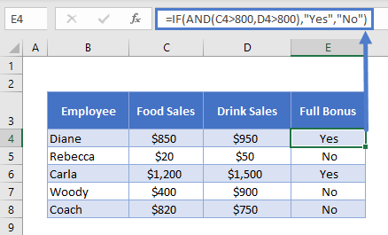

But how would you work out who gets the half bonus? That’s where XOR comes in:

=IF(XOR(C4>=800,D4>=800),"Yes","No")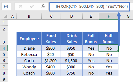

As you can see, Woody’s drink sales were over $800, but not food sales. So he gets the half bonus. The reverse is true for Coach. Diane and Carla sold more than $800 for both, so they don’t get a half bonus (both arguments are TRUE), and Rebecca made under the threshold for both (both arguments FALSE), so the formula again returns “No”.

Using IF with NOT

The NOT Function reverses the outcome of a logical test. In other words, it checks whether a condition has not been met.

You can use it with IF like this:

=IF(AND(C3>=1985,NOT(D3="Steven Spielberg")),"Watch", "Don’t Watch")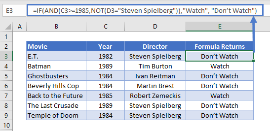

IF NOT

Here we have a table with data on some 1980s movies. We want to identify movies released on or after 1985, that were not directed by Steven Spielberg.

Because NOT is nested within an AND Function, Excel will evaluate that first. It will then use the result as part of the AND.

Nested IF Statements

You can also return an IF statement within your IF statement. This enables you to make more complex calculations.

Let’s go back to our customers table. Imagine you want to classify customers based on their debt level to you:

$0: None
Up to $500: Low
$500 to $1000: Medium
Over $1000: High

You can do this by “nesting” IF statements:

=IF(C4=0,"None",IF(C4<=500,"Low",IF(C4<=1000,"Medium",IF(C4>1000,"High"))))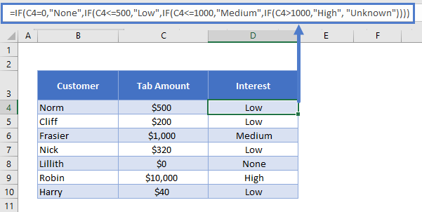

It’s easier to understand if you put the IF statements on separate lines (ALT + ENTER on Windows, CTRL + COMMAND + ENTER on Macs):

=
IF(C4=0,"None",
IF(C4<=500,"Low",
IF(C4<=1000,"Medium",
IF(C4>1000,"High", "Unknown"))))

IF C4 is 0, we return “None”. Otherwise, we move to the next IF statement. IF C4 is equal to or less than 500, we return “Low”. Otherwise, we move on to the next IF statement… and so on.

Simplifying Complex IF Statements with Helper Columns

If you have multiple nested IF statements, and you’re throwing in logic functions too, your formulas can become very hard to read, test, and update.

This is especially important to keep in mind if other people will be using the spreadsheet. What makes sense in your head, might not be so obvious to others.

Helper columns are a great way around this issue.

You’re an analyst in the finance department of a large corporation. You’ve been asked to create a spreadsheet that checks whether each employee is eligible for the company pension.

Here’s the criteria:

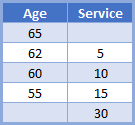
So if you’re under the age of 55, you need to have 30 years’ service under your belt to be eligible. If you’re aged 55 to 59, you need 15 years’ service. And so on, up to age 65, where you’re eligible no matter how long you’ve worked there.

You could use a single, complex IF statement to solve this problem:

=IF(OR(F4>=65,AND(F4>=62,G4>=5),AND(F4>=60,G4>=10),AND(F4>=55,G4>=15),G4>30),"Eligible", "Not Eligible")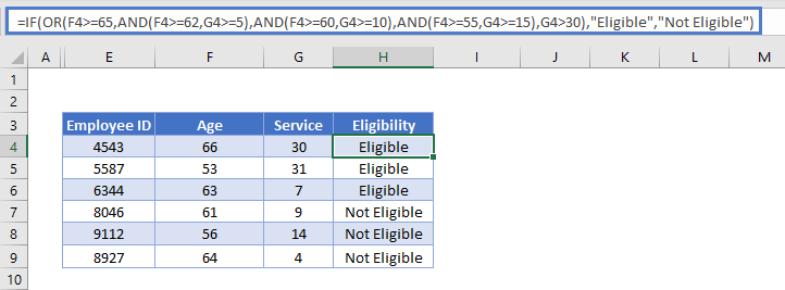

Whew! Kinda hard to get your head around that, isn’t it?

A better approach might be to use helper columns. We have five logical tests here, corresponding to each row in the criteria table. This is easier to see if we add line breaks to the formula, as we discussed earlier:

=IF(
OR(
F4>=65,
AND(F4>=62,G4>=5),
AND(F4>=60,G4>=10),
AND(F4>=55,G4>=15),
G4>30
),"Eligible","Not Eligible")

So, we can split these five tests into separate columns, and then simply check whether any one of them is true:

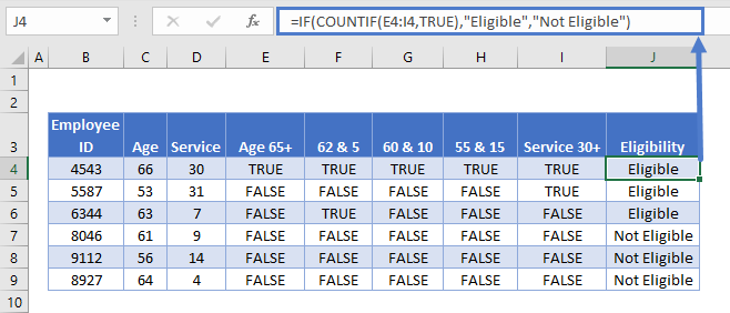
Each column in the table from E to I holds each of our criteria separately. Then in J4 we have the following formula:

=IF(COUNTIF(E4:I4,TRUE),"Eligible","Not Eligible")

Here we have an IF statement, and the logical test uses COUNTIF to count the number of cells within E4:I4 that contain TRUE.

If COUNTIF doesn’t find a TRUE value, it will return 0, which IF interprets as FALSE, so the IF returns “Not Eligible”.

If COUNTIF does find any TRUE values, it will return the number of them. IF interprets any number other than 0 as TRUE, so it returns “Eligible”.

Splitting out the logical tests in this way makes the formula easier to read, and if something’s going wrong with it, it’s much easier to spot where the mistake is.

Using Grouping to Hide Helper Columns

Helper columns make the formula easier to manage, but once you’ve got them in place and you know they are working correctly, they often just take up space on your spreadsheet without adding any useful information.

You could hide the columns, but this can lead to problems because hidden columns are hard to detect, unless you look closely at the column headers.

A better option is grouping.

Select the columns you want to group, in our case E:I. Then press ALT + SHIFT + RIGHT ARROW on Windows, or COMMAND + SHIFT + K on Mac. You can also go to the “Data” tab on the ribbon and select “Group” from the “Outline” section.

You’ll see the group displayed above the column headers, like this:

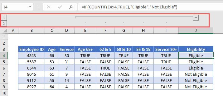
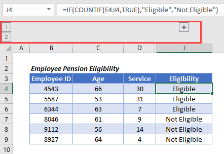
Then simply press the “-“ button to hide the columns:

The IFS Function

Nested IF statements are very useful when you need to perform more complex logical comparisons, and you need to do it in one cell. However, they can get complicated as they get longer, and they can be hard to read and update on your screen.

From Excel 2019 and Excel 365, Microsoft introduced another function, the IFS Function, to help make this a bit easier to manage. The nested IF example above could be achieved with IFS like this:

=IFS(
C4=0,"None",
C4<=500,"Low",
C4<=1000,"Medium",
C4>1000,"High",
TRUE, "Unknown",
)

You can read all about it on the main page for the Excel IFS Function <<link>>.

Using IF with Conditional Formatting

Excel’s Conditional Formatting feature enables you to format a cell in different ways depending on its contents. Since the IF returns different values based on our logical test, we might want to use Conditional Formatting with the IF Function to make these different values easier to see.

So let’s go back to our staff bonus table from earlier.

We’re returning “Yes” or “No” depending on what bonus we want to give. This tells us what we need to know, but the information doesn’t jump out at us. Let’s try to fix that.

Here’s how you’d do it:

Select the cell range containing your IF statements. In our case that’s E4:F8.
Click “Conditional Formatting” on the “Styles” section of the “Home” tab on the ribbon.
Click “Highlight Cells Rules” and then “Equal to”.
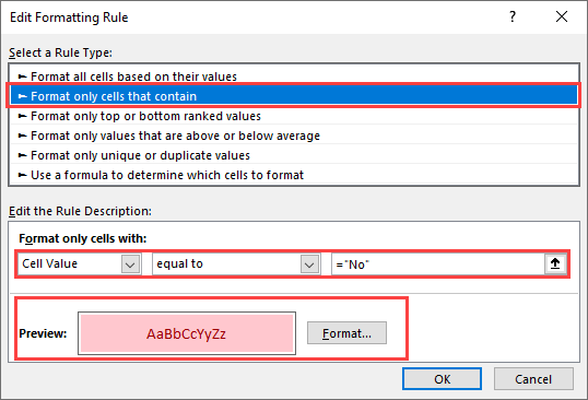
Type “Yes” (or whatever return value you need) into the first box, and then choose the formatting you want from the second box. (I’ll choose green for this).
Repeat for all your return values (I’ll also set “No” values to red)

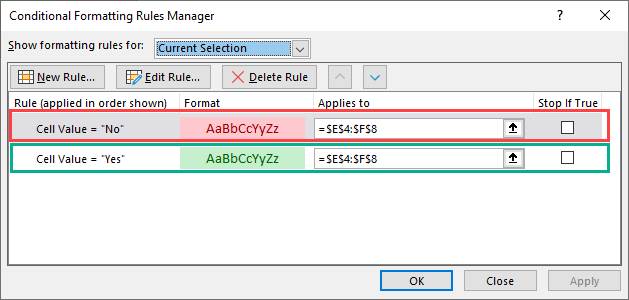
Here’s the result:

Using IF in Array Formulas

An array is a range of values, and in Excel arrays are represented as comma separated values enclosed in braces, such as:

{1,2,3,4,5}

The beauty of arrays, is that they enable you to perform a calculation on each value in the range, and then return the result. For example, the SUMPRODUCT Function takes two arrays, multiplies them together, and sums the results.

So this formula:

=SUMPRODUCT({1,2,3},{4,5,6})

…returns 32. Why? Let’s work it through:

1 * 4 = 4
2 * 5 = 10
3 * 6 = 18

4 + 10 + 18 = 32

We can bring an IF statement into this picture, so that each of these multiplications only happens if a logical test returns true.

For example, take this data:

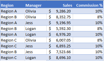
If you wanted to calculate the total commission for each sales manager, you’d use the following:

=SUMPRODUCT(IF($C$2:$C$10=$G2,$D$2:$D$10*$E$2:$E$10))

Note: In Excel 2019 and earlier, you have to press CTRL + SHIFT + ENTER to turn this into an array formula.

We’d end up with something like this:

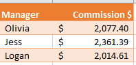
Breaking this down, the “Manager” column is column C, and in this example, Olivia’s name is in G2.

So the logical test is:

$C$2:$C$10=$G2

In English, if the name in column C is equal to what’s in G2 (“Olivia”), DO multiply the values in columns D and E for that row. Otherwise, don’t multiply them. Then, sum all the results.

You can learn more about this formula on the main page for the SUMPRODUCT IF Formula.

IF in Google Sheets

The IF Function works exactly the same in Google Sheets as in Excel:

VBA IF Statements

You can also use If Statements in VBA. Click the link to learn more, but here is a simple example:

Sub Test_IF ()

If Range("a1").Value < 0 then
  Range("b1").Value = "Negative"
End If

End Sub

This code will test if a cell value is negative. If so, it will write “negative” in the next cell.

Источник

How to use Excel If Statement with Multiple Conditions Range [AND/OR]

Excel If Statement Multiple Conditions range

1) Excel If Statement

2) Nested If Statement

3) Excel If with Logical Test

How to apply IF & AND function in Excel

How to use If with Or function in Excel

How to Use If with And & Or function

4) Excel If Statement with other functions

VBA Named Range most efficient way to check if name exists

named range using an if statement with array formula for dependent dropdown

2 Answers 2

How to Create Named Ranges in Excel (A Step-by-step Guide)

Named Ranges in Excel – An Introduction

Benefits of Creating Named Ranges in Excel

Use Names instead of Cell References

No Need to Go Back to the Dataset to Select Cells

Named Ranges Make Formulas Dynamic

How to Create Named Ranges in Excel

Method #1 – Using Define Name

Method #2: Using the Name Box

Method #3: Using Create From Selection Option

Naming Convention for Named Ranges in Excel

Too Many Named Ranges in Excel? Don’t Worry

Getting the Names of All the Named Ranges

Displaying the Matching Named Ranges

How to Edit Named Ranges in Excel

Useful Named Range Shortcuts (the Power of F3)

Creating Dynamic Named Ranges in Excel

How does Dynamic Named Ranges Work?

1) Excel If Statement

2) Nested If Statement

3) Excel If with Logical Test

How to apply IF & AND function in Excel

How to use If with Or function in Excel

How to Use If with And & Or function

4) Excel If Statement with other functions

Nested IF statements based on multiple ranges

Nested IF Statement Using Date Ranges

Nested IF Statements For A Range Of Cells

Nested IF Statement between different values

Named Ranges in Excel – An Introduction

Benefits of Creating Named Ranges in Excel

Use Names instead of Cell References

No Need to Go Back to the Dataset to Select Cells

Named Ranges Make Formulas Dynamic

How to Create Named Ranges in Excel

Method #1 – Using Define Name

Method #2: Using the Name Box

Method #3: Using Create From Selection Option

Naming Convention for Named Ranges in Excel

Too Many Named Ranges in Excel? Don’t Worry

Getting the Names of All the Named Ranges

Displaying the Matching Named Ranges

How to Edit Named Ranges in Excel

Useful Named Range Shortcuts (the Power of F3)

Creating Dynamic Named Ranges in Excel

How does Dynamic Named Ranges Work?

Question

Answers

IF Function Overview

How to Use the IF Function

What can IF Return?

Using IF with AND

Using IF with OR

Using IF with XOR

Using IF with NOT

Nested IF Statements

Simplifying Complex IF Statements with Helper Columns

Using Grouping to Hide Helper Columns

The IFS Function

Using IF with Conditional Formatting

Using IF in Array Formulas

IF in Google Sheets

VBA IF Statements