
The IF function allows you to make a logical comparison between a value and what you expect by testing for a condition and returning a result if that condition is True or False.
-
=IF(Something is True, then do something, otherwise do something else)
But what if you need to test multiple conditions, where let’s say all conditions need to be True or False (AND), or only one condition needs to be True or False (OR), or if you want to check if a condition does NOT meet your criteria? All 3 functions can be used on their own, but it’s much more common to see them paired with IF functions.
Use the IF function along with AND, OR and NOT to perform multiple evaluations if conditions are True or False.
Syntax
-
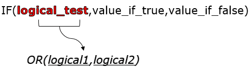
IF(AND()) — IF(AND(logical1, [logical2], …), value_if_true, [value_if_false]))
-
IF(OR()) — IF(OR(logical1, [logical2], …), value_if_true, [value_if_false]))
-
IF(NOT()) — IF(NOT(logical1), value_if_true, [value_if_false]))
|
Argument name |
Description |
|
|
logical_test (required) |
The condition you want to test. |
|
|
value_if_true (required) |
The value that you want returned if the result of logical_test is TRUE. |
|
|
value_if_false (optional) |
The value that you want returned if the result of logical_test is FALSE. |
|
Here are overviews of how to structure AND, OR and NOT functions individually. When you combine each one of them with an IF statement, they read like this:
-
AND – =IF(AND(Something is True, Something else is True), Value if True, Value if False)
-
OR – =IF(OR(Something is True, Something else is True), Value if True, Value if False)
-
NOT – =IF(NOT(Something is True), Value if True, Value if False)
Examples
Following are examples of some common nested IF(AND()), IF(OR()) and IF(NOT()) statements. The AND and OR functions can support up to 255 individual conditions, but it’s not good practice to use more than a few because complex, nested formulas can get very difficult to build, test and maintain. The NOT function only takes one condition.

Here are the formulas spelled out according to their logic:
|
Formula |
Description |
|---|---|
|
=IF(AND(A2>0,B2<100),TRUE, FALSE) |
IF A2 (25) is greater than 0, AND B2 (75) is less than 100, then return TRUE, otherwise return FALSE. In this case both conditions are true, so TRUE is returned. |
|
=IF(AND(A3=»Red»,B3=»Green»),TRUE,FALSE) |
If A3 (“Blue”) = “Red”, AND B3 (“Green”) equals “Green” then return TRUE, otherwise return FALSE. In this case only the first condition is true, so FALSE is returned. |
|
=IF(OR(A4>0,B4<50),TRUE, FALSE) |
IF A4 (25) is greater than 0, OR B4 (75) is less than 50, then return TRUE, otherwise return FALSE. In this case, only the first condition is TRUE, but since OR only requires one argument to be true the formula returns TRUE. |
|
=IF(OR(A5=»Red»,B5=»Green»),TRUE,FALSE) |
IF A5 (“Blue”) equals “Red”, OR B5 (“Green”) equals “Green” then return TRUE, otherwise return FALSE. In this case, the second argument is True, so the formula returns TRUE. |
|
=IF(NOT(A6>50),TRUE,FALSE) |
IF A6 (25) is NOT greater than 50, then return TRUE, otherwise return FALSE. In this case 25 is not greater than 50, so the formula returns TRUE. |
|
=IF(NOT(A7=»Red»),TRUE,FALSE) |
IF A7 (“Blue”) is NOT equal to “Red”, then return TRUE, otherwise return FALSE. |
Note that all of the examples have a closing parenthesis after their respective conditions are entered. The remaining True/False arguments are then left as part of the outer IF statement. You can also substitute Text or Numeric values for the TRUE/FALSE values to be returned in the examples.
Here are some examples of using AND, OR and NOT to evaluate dates.

Here are the formulas spelled out according to their logic:
|
Formula |
Description |
|---|---|
|
=IF(A2>B2,TRUE,FALSE) |
IF A2 is greater than B2, return TRUE, otherwise return FALSE. 03/12/14 is greater than 01/01/14, so the formula returns TRUE. |
|
=IF(AND(A3>B2,A3<C2),TRUE,FALSE) |
IF A3 is greater than B2 AND A3 is less than C2, return TRUE, otherwise return FALSE. In this case both arguments are true, so the formula returns TRUE. |
|
=IF(OR(A4>B2,A4<B2+60),TRUE,FALSE) |
IF A4 is greater than B2 OR A4 is less than B2 + 60, return TRUE, otherwise return FALSE. In this case the first argument is true, but the second is false. Since OR only needs one of the arguments to be true, the formula returns TRUE. If you use the Evaluate Formula Wizard from the Formula tab you’ll see how Excel evaluates the formula. |
|
=IF(NOT(A5>B2),TRUE,FALSE) |
IF A5 is not greater than B2, then return TRUE, otherwise return FALSE. In this case, A5 is greater than B2, so the formula returns FALSE. |

Using AND, OR and NOT with Conditional Formatting
You can also use AND, OR and NOT to set Conditional Formatting criteria with the formula option. When you do this you can omit the IF function and use AND, OR and NOT on their own.
From the Home tab, click Conditional Formatting > New Rule. Next, select the “Use a formula to determine which cells to format” option, enter your formula and apply the format of your choice.

Using the earlier Dates example, here is what the formulas would be.

|
Formula |
Description |
|---|---|
|
=A2>B2 |
If A2 is greater than B2, format the cell, otherwise do nothing. |
|
=AND(A3>B2,A3<C2) |
If A3 is greater than B2 AND A3 is less than C2, format the cell, otherwise do nothing. |
|
=OR(A4>B2,A4<B2+60) |
If A4 is greater than B2 OR A4 is less than B2 plus 60 (days), then format the cell, otherwise do nothing. |
|
=NOT(A5>B2) |
If A5 is NOT greater than B2, format the cell, otherwise do nothing. In this case A5 is greater than B2, so the result will return FALSE. If you were to change the formula to =NOT(B2>A5) it would return TRUE and the cell would be formatted. |
Note: A common error is to enter your formula into Conditional Formatting without the equals sign (=). If you do this you’ll see that the Conditional Formatting dialog will add the equals sign and quotes to the formula — =»OR(A4>B2,A4<B2+60)», so you’ll need to remove the quotes before the formula will respond properly.
Need more help?

See also
You can always ask an expert in the Excel Tech Community or get support in the Answers community.
Learn how to use nested functions in a formula
IF function
AND function
OR function
NOT function
Overview of formulas in Excel
How to avoid broken formulas
Detect errors in formulas
Keyboard shortcuts in Excel
Logical functions (reference)
Excel functions (alphabetical)
Excel functions (by category)
To perform complicated and powerful data analysis, you need to test various conditions at a single point in time. The data analysis might require logical tests also within these multiple conditions.
For this, you need to perform Excel if statement with multiple conditions or ranges that include various If functions in a single formula.
Those who use Excel daily are well versed with Excel If statement as it is one of the most-used formula. Here you can check various Excel If or statement, Nested If, AND function, Excel IF statements, and how to use them. We have also provided a VIDEO TUTORIAL for different If Statements.
There are various If statements available in Excel. You have to know which of the Excel If you will work at what condition. Here you can check multiple conditions where you can use Excel If statement.
1) Excel If Statement
If you want to test a condition to get two outcomes then you can use this Excel If statement.
=If(Marks>=40, “Pass”)
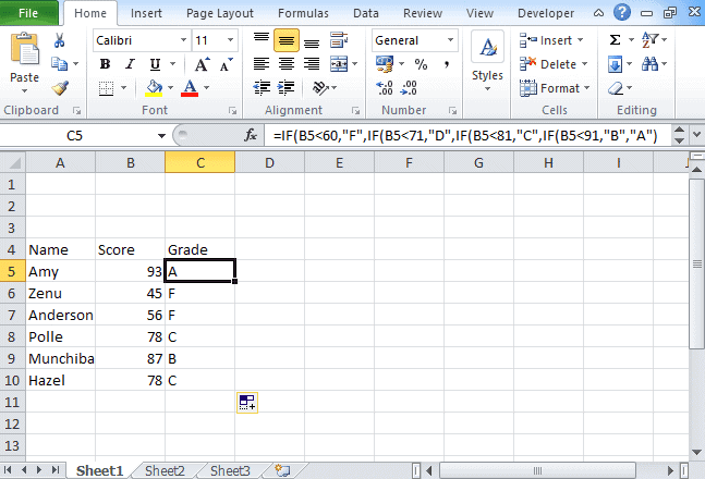
2) Nested If Statement
Let’s take an example that met the below-mentioned condition
- If the score is between 0 to 60, then Grade F
- If the score is between 61 to 70, then Grade D
- If the score is between 71 to 80, then Grade C
- If the score is between 81 to 90, then Grade B
- If the score is between 91 to 100, then Grade A
Then to test the condition the syntax of the formula becomes,
=If(B5<60, “F”,If(B5<71, “D”, If(B5<81,”C”,If(B5<91,”B”,”A”)
3) Excel If with Logical Test
There are 2 different types of conditions AND and OR. You can use the IF statement in excel between two values in both these conditions to perform the logical test.
AND Function: If you are performing the logical test based on AND function, then excel will give you TRUE as an outcome in every condition else it will return false.
OR Function: If you are using OR condition for the logical test, then excel will give you an outcome as TRUE if any of the situations match else it returns false.
For this, multiple testing is to be done using AND and OR function, you should gain expertise in using either or both of these with IF statement. Here we have used if the function with 3 conditions.
How to apply IF & AND function in Excel
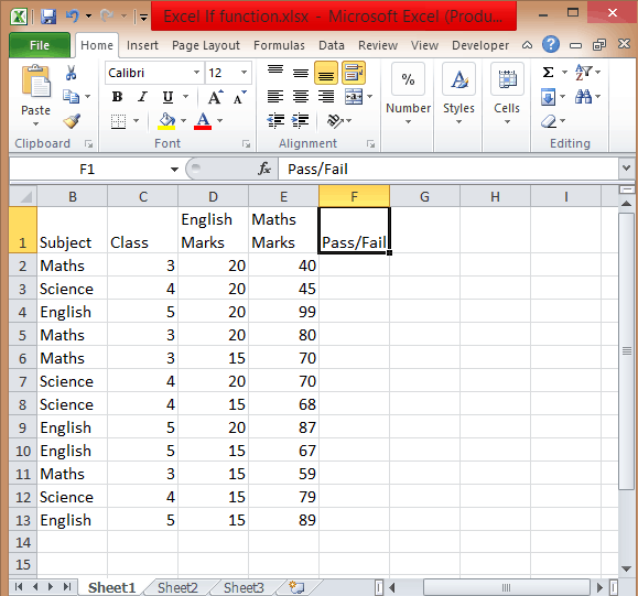
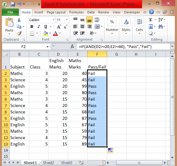
- To perform this multiple if and statements in excel, we will take the data set for the student’s marks that contain fields such as English and Math’s Marks.
- The score of the English subject is stored in the D column whereas the Maths score is stored in column E.
- Let say a student passes the class if his or her score in English is greater than or equal to 20 and he or she scores more than 60 in Maths.
- To create a report in matters of seconds, if formula combined with AND can suffice.
- Type =IF( Excel will display the logical hint just below the cell F2. The parameters of this function are logical_test, value_if_true, value_if_false.
- The first parameter contains the condition to be matched. You can use multiple If and AND conditions combined in this logical test.
- In the second parameter, type the value that you want Excel to display if the condition is true. Similarly, in the third parameter type the value that will be displayed if your condition is false.

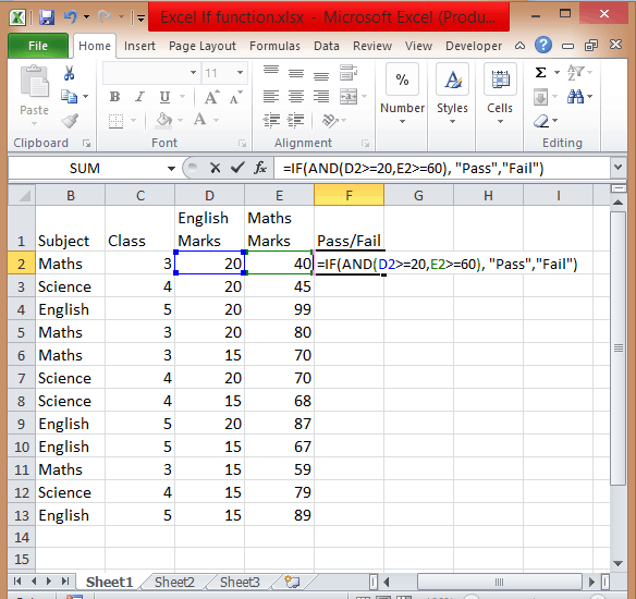
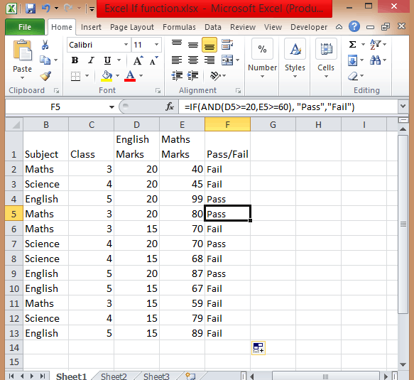
- Apply If & And formula, you will get =IF(AND(D2>=20,E2>=60),”Pass”,”Fail”).
![]()
- Add Pass/Fail column in the current table.

- After you have applied this formula, you will find the result in the column.
- Copy the formula from cell F2 and paste in all other cells from F3 to F13.

How to use If with Or function in Excel
To use If and Or statement excel, you need to apply a similar formula as you have applied for If & And with the only difference is that if any of the condition is true then it will show you True.
To apply the formula, you have to follow the above process. The formula is =IF((OR(D2>=20, E2>=60)), “Pass”, “Fail”). If the score is equal or greater than 20 for column D or the second score is equal or greater than 60 then the person is the pass.
How to Use If with And & Or function
If you want to test data based on several multiple conditions then you have to apply both And & Or functions at a single point in time. For example,
Situation 1: If column D>=20 and column E>=60
Situation 2: If column D>=15 and column E>=60
If any of the situations met, then the candidate is passed, else failed. The formula is
=IF(OR(AND(D2>=20, E2>=60), AND(D2>=20, E2>=60)), “Pass”, “Fail”).
4) Excel If Statement with other functions
Above we have learned how to use excel if statement multiple conditions range with And/Or functions. Now we will be going to learn Excel If Statement with other excel functions.
- Excel If with Sum, Average, Min, and Max functions
Let’s take an example where we want to calculate the performance of any student with Poor, Satisfactory, and Good.
If the data set has a predefined structure that will not allow any of the modifications. Then you can add values with this If formula:
=If((A2+B2)>=50, “Good”, If((A2+B2)=>30, “Satisfactory”, “Poor”))
Using the Sum function,
=If(Sum(A2:B2)>=120, “Good”, If(Sum(A2:B2)>=100, “Satisfactory”, “Poor”))
Using the Average function,
=If(Average(A2:B2)>=40, “Good”, If(Average(A2:B2)>=25, “Satisfactory”, “Poor”))
Using Max/Min,
If you want to find out the highest scores, using the Max function. You can also find the lowest scores using the Min function.
=If(C2=Max($C$2:$C$10), “Best result”, “ “)
You can also find the lowest scores using the Min function.
=If(C2=Min($C$2:$C$10), “Worst result”, “ “)
If we combine both these formulas together, then we get
=If(C2=Max($C$2:$C$10), “Best result”, If(C2=Min($C$2:$C$10), “Worst result”, “ “))
You can also call it as nested if functions with other excel functions. To get a result, you can use these if functions with various different functions that are used in excel.
So there are four different ways and types of excel if statements, that you can use according to the situation or condition. Start using it today.
So this is all about Excel If statement multiple conditions ranges, you can also check how to add bullets in excel in our next post.
I hope you found this tutorial useful
You may also like the following Excel tutorials:
- Multiple If Statements in Excel
- Excel Logical test
- How to Compare Two Columns in Excel (using VLOOKUP & IF)
- Using IF Function with Dates in Excel (Easy Examples)
I received a lot of questions on how to use IF function with 3 conditions, so I’ve decided to write an article on this topic.
The IF examples described in this article assume that you have a basic understanding of how the IF function works. All examples from this article work in Excel for Microsoft 365 or Excel 2021, 2019, 2016, 2013, 2010, and 2007.
IF is one of the most used Excel functions. In case you are unfamiliar with the IF function, then I strongly recommend reading my article on Excel IF function first. It’s a step-by-step guide, and it includes a lot of useful examples. It also shows the basics of writing an Excel IF statement with multiple conditions, but it’s not as detailed as this guide. Make sure you also download the exercise file.
As a data analyst, you need to be able to evaluate multiple conditions at the same time and perform an action or display certain values when the logical tests are TRUE. This means that you will need to learn how to write more complex formulas, which sooner or later will include multiple IF statements in Excel, nested one inside the other.
Let’s take a look at how to write a simple IF function with 3 logical tests.
The first example uses an IF statement with three OR conditions. We will use an IF formula which sets the Finance division name if the department is Accounting, Financial Reporting, or Planning & Budgeting.
The IF statement from cell E31 is:=IF(OR(D31="Accounting", D31="Financial Reporting", D31="Planning & Budgeting"), "Finance", "Other")

This IF formula works by checking three OR conditions:
- Is the data from the cell
D31equal toAccounting? In our case, the answer is no, and the formula continues and evaluates the second condition. - Is the text from the cell
D31equal toFinancial Reporting? The answer is still no, and the formula continues and evaluates the third condition. - Is the text from the cell
D31equal toPlanning & Reporting? The answer is yes, our IF function returns TRUE, and displays the word Finance in cell E31.
Next, we focus our attention on an example that uses an IF statement with three AND conditions.
Our table shows exam scores for three exams. If the student received a score of at least 70 for all three exams, then we will return Pass. Otherwise, we will display Fail.
The IF statement from cell H53 is:=IF(AND(E53>=70, F53>=70, G53>=70), "Pass", "Fail")

This IF formula works by checking all three AND conditions:
- Is the score for Exam 1
higher than or equal to 70? In our case, the answer is yes, and the formula continues and evaluates the second condition. - Is the score for Exam 2
higher than or equal to 70? Well, yes it is. Now the formula moves to the third condition. - Is the score for Exam 3 higher than or equal to 70? Yes, it is. Since all three conditions are met, the IF statement is TRUE and returns the word Pass in cell H53.
Excel IF statement with multiple conditions
The final section of this article is focused on how to write an Excel IF statement with multiple conditions, and it includes two examples:
- multiple nested IF statements (also known as nested IFS)
- formula with a mix of AND, OR, and NOT conditions
How many IF statements can you nest in Excel? The answer is 64, but I’ve never seen a formula that uses that many. Also, I’m sure that there are far better alternatives to using such a complicated formula.
Multiple nested IF statements
In this example, I have calculated the grade of the students based on their scores using a formula with 4 nested IF functions.
=IF(E107<60, "F", IF(E107<70, "D", IF(E107<80, "C", IF(E107<90, "B" ,"A"))))
Note: In this case, the order of the conditions influences the result of your formula. When your conditions overlap, Excel will return the [value_if_true] argument from the first IF statement that is TRUE and ignores the rest of the values. If you want your formula to work properly, always pay attention to the logical flow and the order of your nested IF functions.
If you have to write an IF statement with 3 outcomes, then you only need to use one nested IF function. The first IF statement will handle the first outcome, while the second one will return the second and the third possible outcomes.

Note: If you have Office 365 installed, then you can also use the new IFS function. You can read more about IFS on Microsoft’s website.
Multiple IF statements in Excel with AND, OR, and NOT conditions
I have saved the best for last. This example is the most advanced from this article, as it involves an IF statement with several other logical functions.
In the exercise file, I have included a list of orders. Each row includes the order date, the order value, the product category, and the free shipping flag. We want to flag orders as eligible if the following cumulative logical conditions are met:
- the order was placed during
2020 - the order includes products from only two categories:
PCorLaptop - the order was
notflagged asFree shipping
The formula I’ve used for cell H80 is shown below:
=IF(AND(D80>=DATE(2020,1,1), D80<=DATE(2020,12,31), OR(F80="PC", F80="Laptop"), NOT(G80="Yes")), "Eligible", "Not eligible")

Here’s how this works:
ANDmakes sure that all the logical conditions need to be met to flag the order as Eligible. If any of them is FALSE, then our entire IF statement will return the [value_if_false] argument.D80>=DATE(2020,1,1)andD80<=DATE(2020,12,31)check if the order was placed between January 1st and December 31st, 2020.ORis used to check whether the product category isPCorLaptop.- Finally,
NOTis used to check if the Free shipping flag is different fromYes.
I’ve also added a video that shows how to nest IF functions in case you are still having difficulties understanding how a nested IF formula works.
And there you have it. I hope that after reading this guide, you have a much better understanding of using IF function with 3 logical tests (or any number actually). While it may seem intimidating at first, I guarantee that if you write an IF formula with multiple criteria daily, your productivity will eventually skyrocket.
This is why, if you have any questions on how to use IF function with 3 conditions, please leave a comment below and I will do my best to help you out. I reply to every comment or email that I receive.
In this tutorial, we will learn about the IF function in Excel. Along with IF, the AND and OR functions are important formulas too. A nested IF simply means multiple IF functions in a single syntax.
Introducing IF Function in Excel
Let’s get started with this easy guide to using the IF function and all its related functions in Microsoft Excel, step-by-step with supporting images and examples.
1. IF Function
To learn to use the IF function, we will take an example of a mark list of students below.

Our goal is to find out which student has passed or failed and what are their grades. Of course, it would be a tedious task to find out pass or fail results and grades for each student in this list.
To ease our task, we have IF functions for that matter. The IF function will automatically identify if a student has passed or failed based on the criteria you provide to it.
It will automatically mark a student as “Pass” if he/she has scored above the minimum pass mark and mark a student as “Fail” if he/she has scored below the minimum pass mark.
The IF function automatically assigns the appropriate grades to students based on their marks if you command it.
Here is a glimpse of how the IF function helps you out with assigning grades and marking “Pass” or “Fail”.

Steps to use IF function in Excel
We have allotted certain grades and marked them as Pass or Fail to students based on the percentages they have secured in their exams, with the help of the IF function.
1. Using the IF function in Excel to identify passed/failed students
Let’s learn how we can use the IF formula to achieve this. We will use the same example. We take the minimum passing percentage as 34%.

- Find out the percentage of total marks of every student.
- Create a new column named “Pass/Fail”.
- In the blank cell below the title, type the IF formula as follows next.
- Type =IF( and select the first student’s percentage and type >=34.
- Put a comma and move to the next argument named [value_if_true]. This means you’re being asked to put a value to be displayed if the above condition is true. Remember these arguments are case sensitive.
- Once you have put a comma, type “Pass”.
- Put a comma and move to the next argument named [value_if_false] to display a value when the above condition is false. This field is optional in most cases but we need a false value because it is a mark list.
- Close the bracket and hit ENTER.

You can see that the formula is displaying “Pass” for the first student because she has secured above 34%.
- Double-click or drag the cell from the right corner below to autofill the formula to all the students below.

Recommended read: How to Autofill in Excel?
2. Nested IF Function
Now, let us start assigning grades to all students.
We are going to be using multiple IF functions in a single syntax this time to provide multiple criteria to the IF function. This is called Nested IF in Excel.
However, there is no specific function named “Nested IF” in Excel, it is simply that this behavior has been given a name i.e., Nested IF.
Before we proceed further, we need to first make a table that displays a grading class for each grade. Here is an example below.

- Create a new column named “Grade”.
- Type the IF function in a blank cell below the title as follows.
- Type =IF( and now type AE118>=85,”A”,IF(AE118>=70,”B”,IF(AE118>=55,”C”,IF(AE118>=34,”D”,IF(AE118<=33,”Fail”.

- Note that AE118 is our cell address for the first student’s percentage. It will be different in your case. Refer to the image above to make sense of the formula.
- The formula simply states- if percentage marks are above and equal to 85 then give “A”, if percentage marks are above and equal to 70 then give “B”, and so on and so forth. For the last condition, we have applied the condition- if the marks are less than or equal to 33 then give “Fail”.
- For the last IF statement, you can either put the result as “Fail” or “E” as you like.
- Now, note that we will close the formula with 5 brackets for this example as we have used a total of 5 IF formulas.

- Hit ENTER to complete the formula.

You can now see that the formula has been applied to the first entry and the result is B because the student has secured 72.5% which is less than 75%. This means the nested Ifs are working correctly.
- Now drag the cell from the lower right corner to autofill the formula to the rest of the entries.

You can see that we now have grades and pass/fail markings for every student on the list successfully.
3. IF with AND in Excel
Let us learn the IF formula with the AND function in a single syntax with a minor example.

When you have two or more distinct conditions to be used together, you can use the IF function with AND in Excel.
While nested IFs will also work, using AND function will save your time as it is shorter to type. So, let’s get started.
Our goal is to identify currencies with revenues greater than 20,000 and less than 50,000 and mark them as “Good”.
- Type =IF(AND( because we are using the IF with AND function.
- Select the first cell under Revenue, and type >20000.
- Put a comma and select the first cell under Revenue again and type <50000.
- Now, close the bracket to complete the AND function. We’re still working on the IF function so do not put two brackets.
- We come back to the IF function as soon as we close the AND function. Now put the values to be displayed if the condition is true or false.
- Put a comma to move to the argument [value_if_true] and type “Good”.
- You can provide a result in the [value_if_false] argument, but it is completely optional. If nothing is provided then the cells will display FALSE if the condition is false. But if you want the cells to remain blank simply put “” (two double quotation marks) in this argument.
- Close the bracket to complete the IF function as well.

This is how the syntax should look like before pressing ENTER.
- Hit ENTER to view results and drag the cell down to autofill the formula to the rest of the cells.

There are only two such cells for which the condition is true and the result is being displayed as “Good” for them and the rest of the cells are blank. This means the formula is working correctly.
4. IF with OR in Excel
Using the OR function with the IF function will give results for either of the conditions that are true.
- Type =IF(OR(.
- Select the first cell under Revenue and type >=20000.
- Put a comma and select the first cell under Revenue again and type <=50000.
- Now, close the bracket to complete the OR function. We’re still working on the IF function so do not put two brackets.
- Coming back to the IF function, we now put the values to be displayed if the condition is true or false.
- Put a comma to move to the argument [value_if_true] and type “Flag”.
- Put a comma to move to the argument [value_if_false] and type “”.

This is how the syntax should look like before pressing ENTER.
- Close the bracket to complete the OR function and hit ENTER.
- Drag the cell below to get the results for the rest.

The formula is true for all entries and so it is displaying “Flag” for all of them. This is because all the values are either lower than 50,000 or greater than 20,000.
Conclusion
This was all about IF functions and other related functions to the IF function that are AND and OR functions.
Reference: ExcelJet
Home / Excel Formulas / How to Combine IF and OR Functions in Excel
IF Function is one of the most powerful functions in excel. And, the best part is, that you can combine other functions with IF to increase its power.
Combining IF and OR functions is one of the most useful formula combinations in excel. In this post, I’ll show you why we need to combine IF and OR functions. And, why it’s highly useful for you.
Quick Intro
I am sure you have used both of these functions but let me give you a quick intro.
- IF – Use this function to test a condition. It will return a specific value if that condition is true, or else some other specific value if that condition is false.
- OR – Test multiple conditions. It will return true if any of those conditions is true, and false if all of those conditions are false.
The crux of both of the functions is IF function can test only one condition at a time. And, OR function can test multiple conditions but only return true/false. And, if we combine these two functions we can test multiple conditions with OR & return a specific value with IF.
How do IF and OR functions Work?
In the syntax of the IF function, have a logical test argument that we use to specify a condition to test.
IF(logical_test,value_if_true,value_if_false)
And, then it returns a value based on the result of that condition. Now, if we use OR function for that argument and specify multiple conditions for it.
If any of the conditions is true OR will return true and IF will return the specific value. And, if none of the conditions is true OR with return FALSE IF will return another specific value. In this way, we can test more than one value with the IF function. Let’s get into some real-life examples.
Examples
Here I have a table with stock details of two warehouses. Now the thing is I want to update the status in the table.
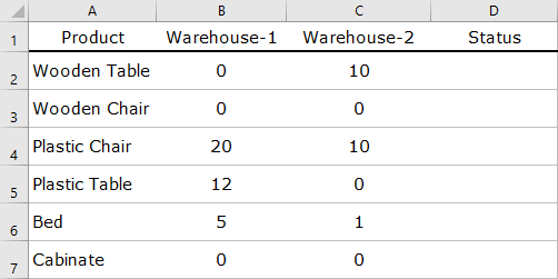
If there is no stock in both of the warehouses status should be “Out of Stock”. And, if there is stock in any of the warehouse status should be “In-Stocks”. So here I have to check two different conditions “Warehouse-1” & “Warehouse-2”.
And the formula will be.
=IF(OR(B2>0,C2>0),"In-Stock","Out of Stock")
In the above formula, if there is a value greater than zero in any of the cells (B2 & C2) OR function will return true, and IF will return the value “In-Stock”. But, if both cells have zero then OR will return false, and IF will return the value “Out of Stock”.
Download Sample File
- Ready
Last Words
Both of the functions are equally useful but when you combine them, you can use them in a better way. As I told you, by combining IF and Or functions you can test more than one condition. You can solve your two problems with this combination of functions.
And, if you want to Get Smarter than Your Colleagues check out these FREE COURSES to Learn Excel, Excel Skills, and Excel Tips and Tricks.
Things will not always be the way we want them to be. The unexpected can happen. For example, let’s say you have to divide numbers. Trying to divide any number by zero (0) gives an error. Logical functions come in handy such cases. In this tutorial, we are going to cover the following topics.
In this tutorial, we are going to cover the following topics.
- What is a Logical Function?
- IF function example
- Excel Logic functions explained
- Nested IF functions
What is a Logical Function?
It is a feature that allows us to introduce decision-making when executing formulas and functions. Functions are used to;
- Check if a condition is true or false
- Combine multiple conditions together
What is a condition and why does it matter?
A condition is an expression that either evaluates to true or false. The expression could be a function that determines if the value entered in a cell is of numeric or text data type, if a value is greater than, equal to or less than a specified value, etc.
IF Function example
We will work with the home supplies budget from this tutorial. We will use the IF function to determine if an item is expensive or not. We will assume that items with a value greater than 6,000 are expensive. Those that are less than 6,000 are less expensive. The following image shows us the dataset that we will work with.
 and conditions in Excel")
- Put the cursor focus in cell F4
- Enter the following formula that uses the IF function
=IF(E4<6000,”Yes”,”No”)
HERE,
- “=IF(…)” calls the IF functions
- “E4<6000” is the condition that the IF function evaluates. It checks the value of cell address E4 (subtotal) is less than 6,000
- “Yes” this is the value that the function will display if the value of E4 is less than 6,000
-
“No” this is the value that the function will display if the value of E4 is greater than 6,000
When you are done press the enter key
You will get the following results
 and conditions in Excel")
Excel Logic functions explained
The following table shows all of the logical functions in Excel
| S/N | FUNCTION | CATEGORY | DESCRIPTION | USAGE |
|---|---|---|---|---|
| 01 | AND | Logical | Checks multiple conditions and returns true if they all the conditions evaluate to true. | =AND(1 > 0,ISNUMBER(1)) The above function returns TRUE because both Condition is True. |
| 02 | FALSE | Logical | Returns the logical value FALSE. It is used to compare the results of a condition or function that either returns true or false | FALSE() |
| 03 | IF | Logical |
Verifies whether a condition is met or not. If the condition is met, it returns true. If the condition is not met, it returns false. =IF(logical_test,[value_if_true],[value_if_false]) |
=IF(ISNUMBER(22),”Yes”, “No”) 22 is Number so that it return Yes. |
| 04 | IFERROR | Logical | Returns the expression value if no error occurs. If an error occurs, it returns the error value | =IFERROR(5/0,”Divide by zero error”) |
| 05 | IFNA | Logical | Returns value if #N/A error does not occur. If #N/A error occurs, it returns NA value. #N/A error means a value if not available to a formula or function. |
=IFNA(D6*E6,0) N.B the above formula returns zero if both or either D6 or E6 is/are empty |
| 06 | NOT | Logical | Returns true if the condition is false and returns false if condition is true |
=NOT(ISTEXT(0)) N.B. the above function returns true. This is because ISTEXT(0) returns false and NOT function converts false to TRUE |
| 07 | OR | Logical | Used when evaluating multiple conditions. Returns true if any or all of the conditions are true. Returns false if all of the conditions are false |
=OR(D8=”admin”,E8=”cashier”) N.B. the above function returns true if either or both D8 and E8 admin or cashier |
| 08 | TRUE | Logical | Returns the logical value TRUE. It is used to compare the results of a condition or function that either returns true or false | TRUE() |
A nested IF function is an IF function within another IF function. Nested if statements come in handy when we have to work with more than two conditions. Let’s say we want to develop a simple program that checks the day of the week. If the day is Saturday we want to display “party well”, if it’s Sunday we want to display “time to rest”, and if it’s any day from Monday to Friday we want to display, remember to complete your to do list.
A nested if function can help us to implement the above example. The following flowchart shows how the nested IF function will be implemented.
 and conditions in Excel")
The formula for the above flowchart is as follows
=IF(B1=”Sunday”,”time to rest”,IF(B1=”Saturday”,”party well”,”to do list”))
HERE,
- “=IF(….)” is the main if function
- “=IF(…,IF(….))” the second IF function is the nested one. It provides further evaluation if the main IF function returned false.
Practical example
 and conditions in Excel")
Create a new workbook and enter the data as shown below
 and conditions in Excel")
- Enter the following formula
=IF(B1=”Sunday”,”time to rest”,IF(B1=”Saturday”,”party well”,”to do list”))
- Enter Saturday in cell address B1
- You will get the following results
 and conditions in Excel")
Download the Excel file used in Tutorial
Summary
Logical functions are used to introduce decision-making when evaluating formulas and functions in Excel.
We learned about IF with AND Function in Excel and IF with OR Function in Excel previously. Now lets use AND function and OR function in one single formula.
Scenario:
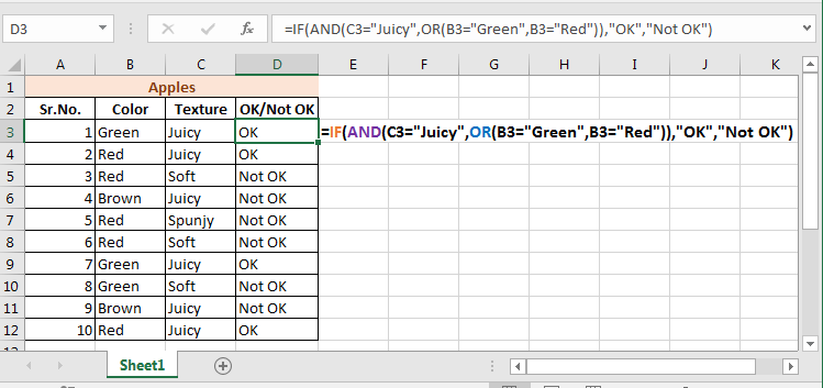
The fruit seller is again here. You would by an apple only if it is Juicy and Red or Green.
So here an apple must be Juicy but in color it can be Red or Green. We need an IF AND OR formula here.
IF This AND That OR That
Generic Formula
=IF(AND(condition1,OR(condition1, condition2,…)),value if true, value if false)
Implementation of IF-AND-OR Formula
So to solve you problem of choosing apple you’ve drawn this table.
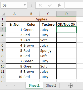
Now to get right apples write this formula in cell D3 and drag it down.
=IF(AND(C3=»Juicy»,OR(B3=»Green»,B3=»Red»)),»OK»,»Not OK»)
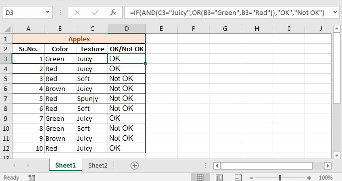
This is the result.
How It Works
It is simple.
OR(B3=»Green»,B3=»Red») : This parts returns TRUE if B3 has Green or Red. Since it is green it returns TRUE.
AND(C3=»Juicy»,OR(B3=»Green»,B3=»Red»): This part becomes AND(C3=»Juicy»,TRUE). AND returns TRUE only if C3 is Juicy and OR returns it TRUE. Since C3 is juicy and OR function has returned TRUE. this part will become AND(TRUE,TRUE). Which will eventually become TRUE.
IF(AND(C3=»Juicy»,OR(B3=»Green»,B3=»Red»)): This part becomes IF(TRUE,”OK”, “Not OK”). As we explained in IF Function article, it will return OK.
So yeah guys, this is the way you can pull conditions like if this and that or that type of conditions without using nested IFs function. Let me know if it was helpful in the comment section.
Related Articles:
IF function with Wildcards
IF with OR Function in Excel
IF with AND Function in Excel
Popular Articles:
50 Excel Shortcut to Increase Your Productivity
The VLOOKUP Function in Excel
COUNTIF in Excel 2016
How to Use SUMIF Function in Excel
Logical functions are designed to test one or several conditions, and perform the actions prescribed for each of the two possible results. Such results can only be logical TRUE or FALSE.
Excel contains several logical functions such as IF, IFERROR, SUMIF, AND, OR, and others. The last two are not used in practice, as a rule, because the result of their calculations may be one of only two possible options (TRUE, FALSE). When combined with the IF function, they are able to significantly expand its functionality.
Examples of using formulas with IF, AND, OR functions in Excel
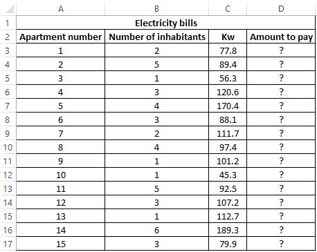
Example 1. When calculating the cost of the amount of consumed kW of electricity for subscribers, the following conditions are taken into account:
- If less than 3 people live in the apartment or less than 100 kW of electricity was consumed per month, the rate per 1 kW is 4.35$.
- In other cases, the rate for 1 kW is 5.25$.
Calculate the amount payable per month for several subscribers.
View source data table:
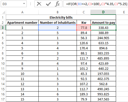
Perform the calculation according to the formula:
Argument Description:
- OR (B3<=2,C3<100) is a logical expression that verifies two conditions: do less than 3 people live in the apartment or does the total amount of energy consumed less than 100 kW? The result of the test will be TRUE if either of these two conditions is true;
- C3 * 4.35 — the amount to be paid, if the OR function returns TRUE;
- C3 * 5.25 is the amount to be paid if OR returns FALSE.
We stretch the formula for the remaining cells using the autocomplete function. The result of the calculation for each subscriber:
Using the AND function in the formula in the first argument in the IF function, we check the conformity of the values by two conditions at once.
Formula with IF and AVERAGE functions for selecting of values by conditions
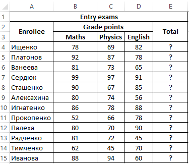
Example 2. Applicants entering the university for the specialty «mechanical engineer» are required to pass 3 exams in mathematics, physics and English. The maximum score for each exam is 100. The average passing score for 3 exams is 75, while the minimum score in physics must be at least 70 points, and in mathematics it is 80. Determine applicants who have successfully passed the exams.
View source table:
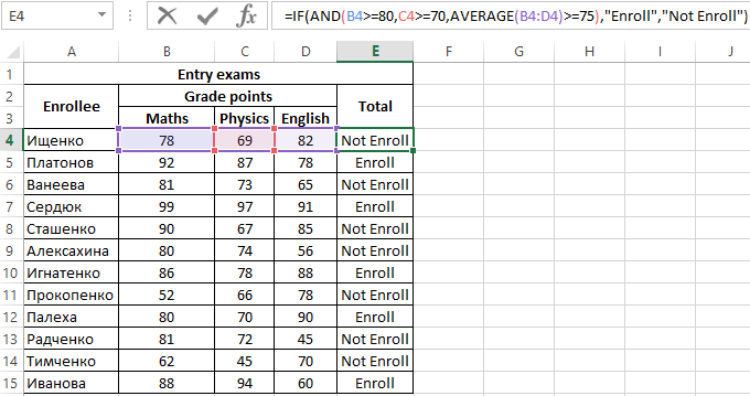
To determine the enrolled students use the formula:
Argument Description:
- AND(B4>=80,C4>=70,AVERAGE(B4:D4)>=75) — checked logical expressions according to the condition of the problem;
- «Enroll» — the result, if the function AND returned the value TRUE (all expressions represented as its arguments, as a result of the calculations returned the value TRUE);
- «Not Enroll» — the result if AND returned FALSE.
Using the autocomplete function (double-click on the cursor marker in the lower right corner), we get the rest of the results:
Formula with logical functions AND IF OR in excel
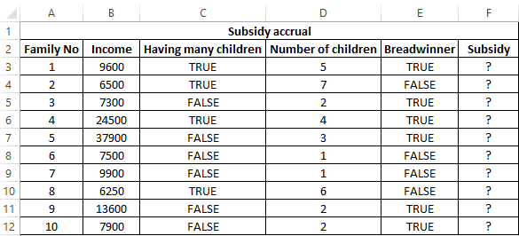
Example 3. Subsidies in the amount of 30% are charged to families with an average income below 8,000$, which are large or there is no main breadwinner. If the number of children is over 5, the amount of the subsidy is 50%. Determine who should receive subsidies and who should not.
View source table:
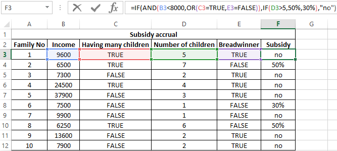
To check the criteria according to the condition of the problem, we write the formula:
Argument Description:
- AND(B3<8000,OR(C3=TRUE,E3=FALSE)) is the checked expression according to the condition of the problem. In this case, the AND function returns the TRUE value, if B3 <8000 is true and at least one of the expressions passed as arguments to the OR function also returns the TRUE value.
- The nested IF function performs a check on the number of children in the family, which rely on subsidies.
- If the main condition returned the result is FALSE, the main function IF returns the text string “no”.
Perform the calculation for the first family and stretch the formula to the remaining cells using the autocomplete function. Results:
Features of using logical functions IF, AND, OR in Excel
The IF function has the following syntax notation:
=IF(Logical_test,[ Value_if_True ],[ Value_if_False])
As you can see, by default, you can check only one condition, for example, is e3 more than 20? Using the IF function, this check can be done as follows:
=IF(EXP(3)>20,»more»,»less»)
As a result, the text string “more” will be returned. If we need to find out if any value belongs to the specified interval, we will need to compare this value with the upper and lower limits of the intervals, respectively. For example, is the result of calculating e3 in the range from 20 to 25? When using the IF function alone, you must enter the following entry:
=IF(EXP(3)>20,IF(EXP(3)<25,»belongs»,»does not belong»),»does not belong»)
We have a nested function IF as one of the possible results of the implementation of the main function IF, and therefore the syntax looks somewhat cumbersome. If you also need to know, for example, whether the square root e3 is equal to a numeric value from a fractional number range from 4 to 5, the final formula will look cumbersome and unreadable.
It is much easier to use as a condition a complex expression that can be written using AND and OR functions. For example, the above function can be rewritten as follows:
=IF(AND(EXP(3)>20,EXP(3)<25),»belongs»,»does not belong»)
The result of the execution of the AND expression (EXP(3)>20,EXP(3)<25) can be a logical value TRUE only if the result of checking each of the specified conditions is a logical value TRUE. In other words, the function AND allows you to test one, two or more hypotheses on their truth, and returns the result FALSE if at least one of them is incorrect.
Sometimes you want to know if at least one assumption is true. In this case, it is convenient to use the OR function, which performs the check of one or several logical expressions and returns a logical TRUE, if the result of the calculations of at least one of them is a logical TRUE. For example, you want to know if e3 is an integer or a number that is less than 100? To test this condition, you can use the following formula:
=IF(OR(MOD(EXP(3),1)<>0,EXP(3)<100),»true»,»false»)
The “<>” means inequality, that is, more or less than some value. In this case, both expressions return the value TRUE, and the result of the execution of the IF function is the text string «true.» However, if an OR test was performed (MOD(EXP (3),1)<>0,EXP(3)<20, while EXP(3) <20 will return FALSE, the result of the calculation of the IF function will not change, since MOD(EXP(3),1) <> 0 returns TRUE.
Download examples using the functions OR AND IF in Excel
In practice, often used bundles IF + AND, IF + OR, or all three functions at once. Consider examples of similar use of these functions.