
Содержание
- IF function
- Simple IF examples
- Common problems
- Need more help?
- How to Find Matching Values in Excel
- What’s An Excel Function?
- The Exact Function
- The MATCH Function
- The VLOOKUP Function
- How Do I Find Matching Values in Two Different Sheets?
- How Else Can I Use These Functions?
- How to Tell if Two Cells in Excel Contain the Same Value
- How to Check for Duplicate Cells using the Exact Function
- How to Use the Exact Excel Function to Check for Duplicates
- How to Check Excel for Duplicate Cells using the IF Function
IF function
The IF function is one of the most popular functions in Excel, and it allows you to make logical comparisons between a value and what you expect.
So an IF statement can have two results. The first result is if your comparison is True, the second if your comparison is False.
For example, =IF(C2=”Yes”,1,2) says IF(C2 = Yes, then return a 1, otherwise return a 2).

Use the IF function, one of the logical functions, to return one value if a condition is true and another value if it’s false.
IF(logical_test, value_if_true, [value_if_false])
The condition you want to test.
The value that you want returned if the result of logical_test is TRUE.
The value that you want returned if the result of logical_test is FALSE.
Simple IF examples

In the above example, cell D2 says: IF(C2 = Yes, then return a 1, otherwise return a 2)

In this example, the formula in cell D2 says: IF(C2 = 1, then return Yes, otherwise return No)As you see, the IF function can be used to evaluate both text and values. It can also be used to evaluate errors. You are not limited to only checking if one thing is equal to another and returning a single result, you can also use mathematical operators and perform additional calculations depending on your criteria. You can also nest multiple IF functions together in order to perform multiple comparisons.
 B2,”Over Budget”,”Within Budget”)» loading=»lazy»>
=IF(C2>B2,”Over Budget”,”Within Budget”)
In the above example, the IF function in D2 is saying IF(C2 Is Greater Than B2, then return “Over Budget”, otherwise return “Within Budget”)
 B2,C2-B2,»»)» loading=»lazy»>
In the above illustration, instead of returning a text result, we are going to return a mathematical calculation. So the formula in E2 is saying IF(Actual is Greater than Budgeted, then Subtract the Budgeted amount from the Actual amount, otherwise return nothing).

In this example, the formula in F7 is saying IF(E7 = “Yes”, then calculate the Total Amount in F5 * 8.25%, otherwise no Sales Tax is due so return 0)
Note: If you are going to use text in formulas, you need to wrap the text in quotes (e.g. “Text”). The only exception to that is using TRUE or FALSE, which Excel automatically understands.
Common problems
What went wrong
There was no argument for either value_if_true or value_if_False arguments. To see the right value returned, add argument text to the two arguments, or add TRUE or FALSE to the argument.
This usually means that the formula is misspelled.
Need more help?
You can always ask an expert in the Excel Tech Community or get support in the Answers community.
Источник
How to Find Matching Values in Excel
Ladies and gentlemen, introducing the Exact function
You’ve got an Excel workbook with thousands of numbers and words. There are bound to be multiples of the same number or word in there. You might need to find them. So we’re going to look at several ways you can find matching values in Excel 365.
We’re going to cover finding the same words or numbers in two different worksheets and in two different columns. We’ll look at using the EXACT, MATCH, and VLOOKUP functions. Some of the methods we’ll use may not work in the web version of Microsoft Excel, but they will all work in the desktop version.
What’s An Excel Function?
If you’ve used functions before, skip ahead.
An Excel function is like a mini app. It applies a series of steps to perform a single task. The most commonly used Excel functions can be found in the Formulas tab. Here we see them categorized by the nature of the function –
- AutoSum
- Recently Used
- Financial
- Logical
- Text
- Date & Time
- Lookup & Reference
- Math & Trig
- More Functions.
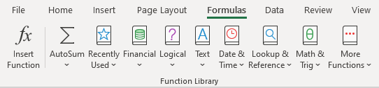
The More Functions category contains the categories Statistical, Engineering, Cube, Information, Compatibility, and Web.
The Exact Function
The Exact function’s task is to go through the rows of two columns and find matching values in the Excel cells. Exact means exact. On its own, the Exact function is case sensitive. It won’t see New York and new york as being a match.
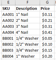
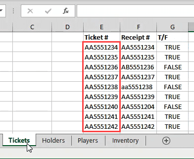
In the example below, there are two columns of text – Tickets and Receipts. For only 10 sets of text, we could compare them by looking at them. Imagine if there were 1,000 rows or more though. That’s when you would use the Exact function.
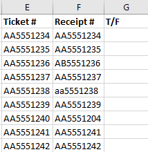
Place the cursor in cell C2. In the formula bar, enter the formula
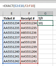
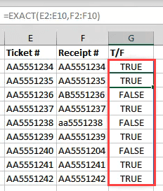
E2:E10 refers to the first column of values and F2:F10 refers to the column right next to it. Once we press Enter, Excel will compare the two values in each row and tell us if it’s a match (True) or not (False). Since we used ranges instead of just two cells, the formula will spill over into the cells below it and evaluate all the other rows.
This method is limited though. It will only compare two cells that are on the same row. It won’t compare what’s in A2 with B3 for example. How do we do that? MATCH can help.
The MATCH Function
MATCH can be used to tell us where a match for a specific value is in a range of cells.
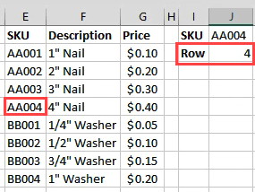
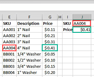
Let’s say we want to find out what row a specific SKU (Stock Keeping Unit) is in, in the example below.
If we want to find what row AA003 is in, we would use the formula:
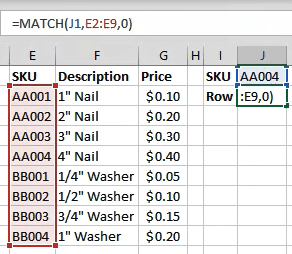
J1 refers to the cell with the value we want to match. E2:E9 refers to the range of values we’re searching through. The zero (0) at the end of the formula tells Excel to look for an exact match. If we were matching numbers, we could use 1 to find something less than our query or 2 to find something greater than our query.
But what if we wanted to find the price of AA003?
The VLOOKUP Function
The V in VLOOKUP stands for vertical. Meaning it can search for a given value in a column. What it can also do is return a value on the same row as the found value.
If you’ve got an Office 365 subscription in the Monthly channel, you can use the newer XLOOKUP. If you only have the semi-annual subscription it will be available to you in July 2020.
Let’s use the same inventory data and try to find the price of something.

Where we were looking for a row before, enter the formula:
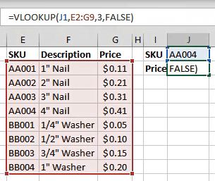
J1 refers to the cell with the value we’re matching. E2:G9 is the range of values we’re working with. But VLOOKUP will only look in the first column of that range for a match. The 3 refers to the 3rd column over from the start of the range.
So when we type a SKU in J1, VLOOKUP will find the match and grab the value from the cell 3 columns over from it. FALSE tells Excel what kind of match we’re looking for. FALSE means it must be an exact match where TRUE would tell it that it has to be a close match.
How Do I Find Matching Values in Two Different Sheets?
Each of the functions above can work across two different sheets to find matching values in Excel. We’re going to use the EXACT function to show you how. This can be done with almost any function. Not just the ones we covered here. There are also other ways to link cells between different sheets and workbooks.
Working on the Holders sheet, we enter the formula
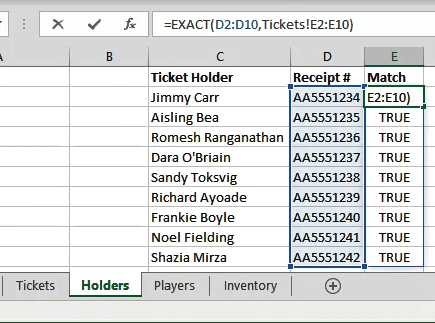
D2:D10 is the range we’ve selected on the Holders sheet. Once we put a comma after that, we can click on the Tickets sheet and drag and select the second range.
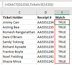
See how it references the sheet and range as Tickets!E2:E10? In this case each row matches, so the results are all True.
How Else Can I Use These Functions?
Once you master these functions for matching and finding things, you can start doing a lot of different things with them. Also take a look at using the INDEX and MATCH functions together to do something similar to VLOOKUP.
Have some cool tips on using Excel functions to find matching values in Excel? Maybe a question about how to do more? Drop us a note in the comments below.
Guy has been published online and in print newspapers, nominated for writing awards, and cited in scholarly papers due to his ability to speak tech to anyone, but still prefers analog watches. Read Guy’s Full Bio
Источник
How to Tell if Two Cells in Excel Contain the Same Value
Many companies still use Excel as it allows them to store different types of data, such as tax records and business contacts. Since many things are often done manually in Excel, there is a potential risk of storing duplicate information. It’s usually not an intentional act; it just happens when entering data with a typo, such as a name, account number, amount, or even an address.
Typos or misspellings often lead to new entries when existing data already exists. For instance, your records may have data for John Doe, Jon Dow, or Jon Dow, even though they are the same person.
Making these kinds of mistakes can sometimes lead to grave consequences. That’s precisely why accuracy is so important when working in spreadsheets. Thankfully, Excel includes features and tools that help everyday users check their data and correct errors.
This article shows you how to check whether two or more Excel cells have the same value.
How to Check for Duplicate Cells using the Exact Function
If you want to check whether or not two or more cells have the same value but don’t want to go through the whole table manually, you can make Excel do the work for you. Excel has a built-in function called “Exact.” This function works for both numbers and text.
How to Use the Exact Excel Function to Check for Duplicates
Let’s say you are working with the worksheet shown in the picture below. As you can see, it isn’t easy to determine whether the numbers from column A are the same as any numbers found in column B. Of course, it’s easier than comparing different cells from each column, but you get the idea.

To ensure that cells from column “A” don’t have a duplicate entry in the corresponding column “B” cells, use the “Exact” function, such as checking cells “A1” and “B1” by adding the formula to cell “C1.”
- Click on the “Formulas” tab, then select the “Text” button.

- Choose “EXACT” from the drop-down menu. The “Exact” formula works on numbers as well.
- A window called “Function Arguments” appears. You need to specify which cells you want to compare.
- To compare cells “A1” and “B1,” type “A1” in the “Text1” box and then “B1” in the “Text2” box, then click “OK.”
- Since the numbers from cells “A1” and “B1” don’t match, Excel returns a “FALSE” value and stores the result in cell “C1.”
- To check all cells, drag the “fill handle” (small square in the bottom-right corner of the cell) down the column as far as needed. This action copies and applies an adjusted formula to all other rows.
- After copying the formula down the column, you should notice that the “FALSE” value appears for non-duplicates in each row, and “TRUE” appears for identical ones.


How to Check Excel for Duplicate Cells using the IF Function
Another function that allows you to check two or more cells for duplicates is the “IF” function. It compares cells from one column, row by row. Let’s use the same two columns (A1 and B1) as in the previous example.
To use the “IF” function correctly, remember its syntax.
- In cell “C1,” type the following formula: =IF(A1=B1, “Match”, “”), and you’ll see “Match” next to the cells that have duplicate entries.
- To check for differences, you should type the following formula: =IF(A1<>B1, “No match”,” “). Again, use the fill handle by dragging it down to apply the function to all cells.
- Excel also allows you to check for duplicates and differences simultaneously by typing the following formula: =IF (A1=B1, “No Match”, “Match“) .


In closing, checking for duplicates in Excel is relatively easy when you implement formulas. The human eyes sometimes overlook identical cells, especially when there are hundreds of them to compare. Also, using formulas builds on efficiency and reduces fatigue, not to mention eye strain. These are the easiest methods to find out whether two cells have the same value in Excel.
Of course, there are times when duplicate cells are valid entries, such as dollar amounts for more than one account, two different family members with the same name, or even repeat transactions. Therefore, check the entries before taking action on them, and make a copy first to prevent data loss if something goes wrong.
Источник
IF function
The IF function is one of the most popular functions in Excel, and it allows you to make logical comparisons between a value and what you expect.
So an IF statement can have two results. The first result is if your comparison is True, the second if your comparison is False.
For example, =IF(C2=”Yes”,1,2) says IF(C2 = Yes, then return a 1, otherwise return a 2).
Use the IF function, one of the logical functions, to return one value if a condition is true and another value if it’s false.
IF(logical_test, value_if_true, [value_if_false])
For example:
-
=IF(A2>B2,»Over Budget»,»OK»)
-
=IF(A2=B2,B4-A4,»»)
|
Argument name |
Description |
|---|---|
|
logical_test (required) |
The condition you want to test. |
|
value_if_true (required) |
The value that you want returned if the result of logical_test is TRUE. |
|
value_if_false (optional) |
The value that you want returned if the result of logical_test is FALSE. |
Simple IF examples
-
=IF(C2=”Yes”,1,2)
In the above example, cell D2 says: IF(C2 = Yes, then return a 1, otherwise return a 2)
-
=IF(C2=1,”Yes”,”No”)
In this example, the formula in cell D2 says: IF(C2 = 1, then return Yes, otherwise return No)As you see, the IF function can be used to evaluate both text and values. It can also be used to evaluate errors. You are not limited to only checking if one thing is equal to another and returning a single result, you can also use mathematical operators and perform additional calculations depending on your criteria. You can also nest multiple IF functions together in order to perform multiple comparisons.
-
=IF(C2>B2,”Over Budget”,”Within Budget”)
In the above example, the IF function in D2 is saying IF(C2 Is Greater Than B2, then return “Over Budget”, otherwise return “Within Budget”)
-
=IF(C2>B2,C2-B2,0)
In the above illustration, instead of returning a text result, we are going to return a mathematical calculation. So the formula in E2 is saying IF(Actual is Greater than Budgeted, then Subtract the Budgeted amount from the Actual amount, otherwise return nothing).
-
=IF(E7=”Yes”,F5*0.0825,0)
In this example, the formula in F7 is saying IF(E7 = “Yes”, then calculate the Total Amount in F5 * 8.25%, otherwise no Sales Tax is due so return 0)
Note: If you are going to use text in formulas, you need to wrap the text in quotes (e.g. “Text”). The only exception to that is using TRUE or FALSE, which Excel automatically understands.
Common problems
|
Problem |
What went wrong |
|---|---|
|
0 (zero) in cell |
There was no argument for either value_if_true or value_if_False arguments. To see the right value returned, add argument text to the two arguments, or add TRUE or FALSE to the argument. |
|
#NAME? in cell |
This usually means that the formula is misspelled. |
Need more help?
You can always ask an expert in the Excel Tech Community or get support in the Answers community.

See Also
IF function — nested formulas and avoiding pitfalls
IFS function
Using IF with AND, OR and NOT functions
COUNTIF function
How to avoid broken formulas
Overview of formulas in Excel
Need more help?
In Excel, there are plenty of formulas you can use to determine if two values are equal. Here are some examples.

Yes, you can tell if two numbers are equal in an instant just by looking at them. But that won’t be the case when you’re looking at larger numbers, or if you want to test multiple numbers in two columns to see if they’re equal.
Like everything else, Excel has a remedy that makes this test easier. There are many formulas you could write that check if two values in Excel are equal or not. Two of the simpler ones consist of the DELTA function and the IF function.
What Is the DELTA Function in Excel?
DELTA is a function in Excel that tests if two numerical values are equal or not. If the two values are equal, DELTA will return 1, and if they are not equal, it will return 0.
=DELTA(number1, number2)
The DELTA function can only operate on numbers, and it cannot test whether two text strings are equal or not. If number2 is left blank, DELTA will assume that it is zero.
How to Test if Two Values Are Equal With the DELTA Function
DELTA can be easily coupled with other Excel functions to count the equal number pairs in a list. In this sample spreadsheet, we have two columns of numbers, and we want to see how many pairs are equal.
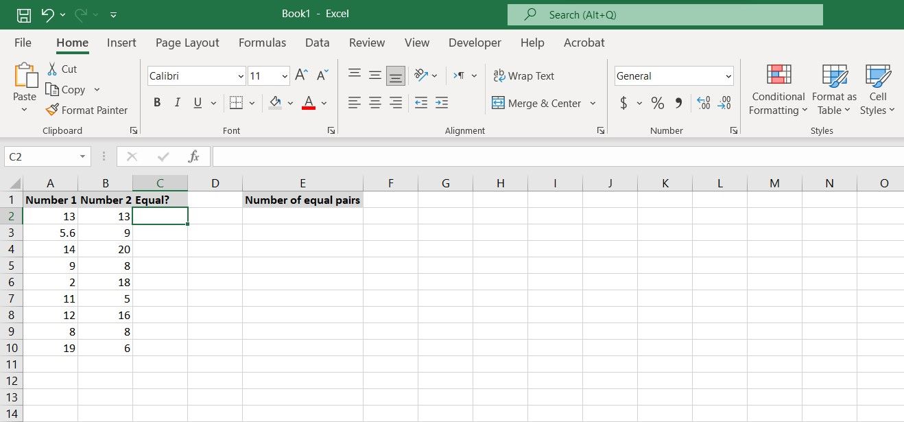
For this example, we’re going to use the DELTA function to check if the numbers in each pair are equal. Then, we’re going to get the count of equal pairs using Excel’s COUNTIF function. Here’s how:
- Select the first cell in the column where you want to check if the numbers are equal. In this example, we’ll use cell C2.
- In the formula bar, enter the formula below:
=DELTA(A2, B2) - Press Enter. DELTA will now tell you if the two numbers are equal or not.
- Grab the fill handle and drop it on the cells below to get the test results for all the numbers.

The formula we used here calls on DELTA to test the numbers in A2 and B2 and see if they’re equal. The formula then returns 1 to indicate that they were equal. If the two numbers weren’t equal, the formula would return 0.
Now you can see which pairs have equal numbers using the DELTA function. Unfortunately, that’s as far as the DELTA function goes. To count the number of pairs with equal numbers, you’ll have to use other functions. One candidate for this task is the COUNTIF function.
COUNTIF can go through a range of cells and return the number of cells that meet a specific condition. Since DELTA returned 1 to indicate equal pairs, we can ask COUNTIF to go through DELTA’s output and count the cells containing 1. This will give us the number of equal pairs.
- Select the cell where you want to show the count of pairs with equal numbers.
- In the formula bar, enter the formula below:
=COUNTIF(C2:C10, "=1") - Press Enter.
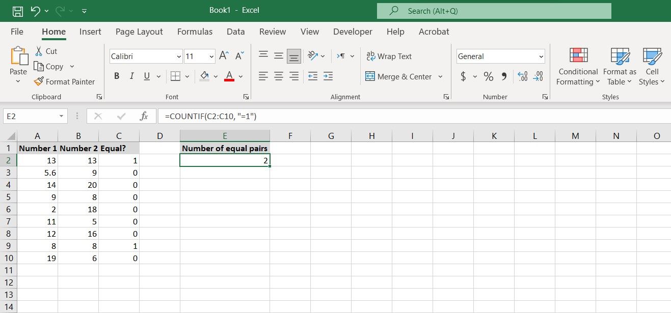
The formula calls on COUNTIF to check the cells C2 to C10 (the results from the DELTA function) and return the number of cells that equal 1.
Remember that the DELTA function returns 1 when the two values are equal, so this formula will count the number of pairs with equal numbers. You can replace 1 with 0 in the formula to get the count of pairs with unequal numbers.
The DELTA function is a simple enough method to check if two numbers are equal. However, if you don’t like the binary output of the DELTA function, you can use the IF function instead to get a custom output.
What Is the IF Function in Excel?
IF is one of the core Excel functions that lets you build sophisticated formulas. It takes a condition and then returns two user-specified outputs if the condition is or is not met.
=IF(logical_Test, Output_If_True, Output_If_False)
The IF function conducts a logical test, and if the test result is true, it returns Output_If_True. Otherwise, it returns Output_If_False.
IF is on a whole other league than DELTA. Where DELTA could only determine whether two numbers are equal, IF can run any kind of logical tests. Another advantage of IF to DELTA is that it isn’t restricted to numbers. In addition to numbers, you can check whether two strings of text are equal using IF in Excel.
How to Test if Two Values Are Equal With the IF Function
In this context, the IF function works in the same way as the DELTA function, except that you can have it output a specific string. To check if two values are equal with the IF function, you need to run a logical test where you put the two cells as equal.
Then, you’ll need to specify outputs for the two scenarios: The test result being true, and the test result being false.
Let’s put the IF function to use in the same example. We’re going to see which numbers pairs are equal, and then count the equal ones using the COUNTIF function.
- Select the first cell in the column where you want to return the test results. This will be cell C2 for this example.
- In the formula bar, enter the formula below:
=IF(A2=B2, "Yes", "No") - Press Enter. The IF function will now tell you whether the two values are equal or not.
- Grab the fill handle and drop it on the cells below. The IF function will now test each pair and return the results accordingly.
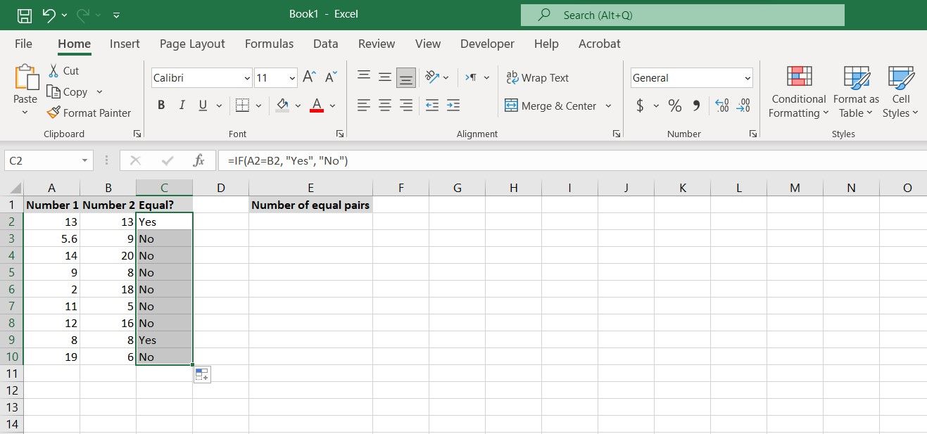
The formula we used will test cells A2 and B2 to see if they’re equal. If the two cells are equal, the formula will return Yes. Otherwise, the formula will return No.
You can count the equal pairs using the COUNTIF function in the same way as the previous example, except that instead of counting the cells that equal 1, you should count the cells containing the string Yes.
This is because the IF formula you wrote returns Yes for pairs that contain equal values. Here’s how you can count the equal pairs:
- Select the cell where you want to return the count. For this example, we’ve chosen cell E2.
- In the formula bar, enter the formula below:
=COUNTIF(C2:C10, "=Yes") - Press Enter. COUNTIF will now tell you how many pairs contain equal values.
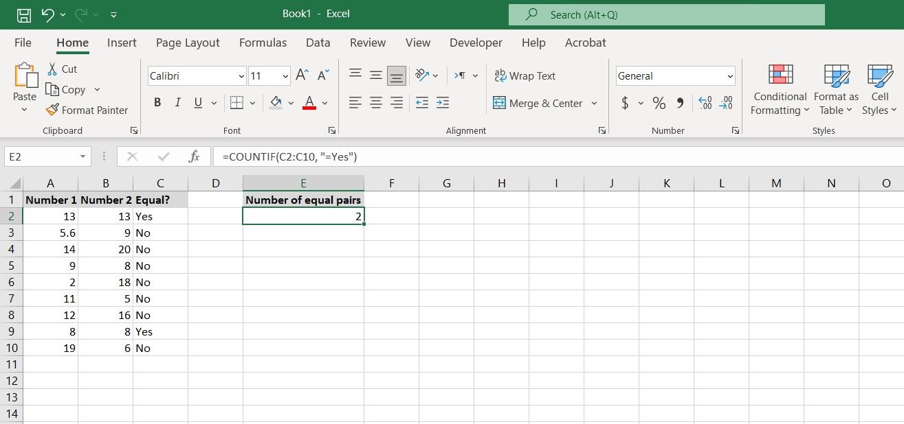
This formula will summon COUNTIF to look through cells C2 to C10 (the results from the IF function) for cells containing the string Yes and then return the count of cells that do.
Since IF returned Yes for equal pairs, then this will be the count of equal pairs.
Test if Two Values Are Equal With Excel Functions
There are plenty of formulas you could write up to check whether two values are equal in Excel. The DELTA function is designed to serve this purpose exclusively, whereas the IF function can accomplish many feats, this included.
Excel exists to take the burden of counting and calculating off your shoulders. This is one minor instance of how Excel can do that, and make your life easier as a result.
Explanation
If you want to do something specific when a cell equals a certain value, you can use the IF function to test the value, then do something if the result is TRUE, and (optionally) do something else if the result of the test is FALSE.
In the example shown, we want to mark rows where the color is red with an «x». In other words, we want to test cells in column B, and take a specific action when they equal the word «red». The formula in cell D6 is:
=IF(B6="red","x","")
In this formula, the logical test is this bit:
B6="red"
This will return TRUE if the value in B6 is «red» and FALSE if not. Since we want to mark or flag red items, we only need to take action when the result of the test is TRUE. In this case, we are simply adding an «x» to column D if when the color is red. If the color is not red (or blank, etc.), we simply return an empty string («»), which displays as nothing.
Note: if an empty string («») is not provided for value_if_false, the formula will return FALSE when the color is not red or green.
Increase price if color is red
Of course, you could do something more complicated as well. For example, let’s say you want to increase the price of red items only by 15%.
In that case, you could use this formula in column E to calculate a new price:
=IF(B6="red",C6*1.15,C6)

The test is the same as before (B6=»red»). If the result is TRUE, we multiply the original price by 1.15 (increase by 15%). If the result of the test is FALSE, we simply use the original price as-is.
When you’re working with data in Excel, sooner or later you will have to compare data. This could be comparing two columns or even data in different sheets/workbooks.
In this Excel tutorial, I will show you different methods to compare two columns in Excel and look for matches or differences.
There are multiple ways to do this in Excel and in this tutorial I will show you some of these (such as comparing using VLOOKUP formula or IF formula or Conditional formatting).
So let’s get started!
Compare Two Columns (Side by Side)
This is the most basic type of comparison where you need to compare a cell in one column with the cell in the same row in another column.
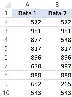
Suppose you have a dataset as shown below and you simply want to check whether the value in column A in a specific cell is the same (or different) when compared with the value in the adjacent cell.
Of course, you can do this when you have a small dataset when you have a large one, you can use a simple comparison formula to get this done. And remember, there is always a chance of human error when you do this manually.
So let me show you a couple of easy ways to do this.
Compare Side by Side Using the Equal to Sign Operator
Suppose you have the below dataset and you want to know what rows have the matching data and what rows have different data.
Below is a simple formula to compare two columns (side by side):
=A2=B2
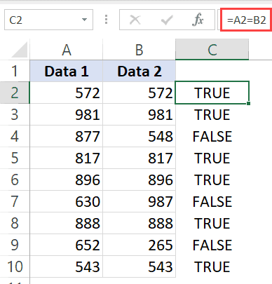
The above formula will give you a TRUE if both the values are the same and FALSE in case they are not.
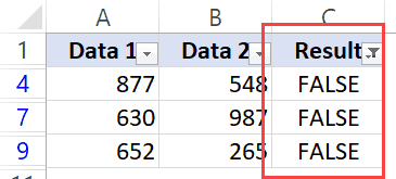
Now, if you need to know all the values that match, simply apply a filter and only show all the TRUE values. And if you want to know all the values that are different, filter all the values that are FALSE (as shown below):
When using this method to do column comparison in Excel, it’s always best to check that your data does not have any leading or trailing spaces. If these are present, despite having the same value, Excel will show them as different. Here is a great guide on how to remove leading and trailing spaces in Excel.
Compare Side by Side Using the IF Function
Another method that you can use to compare two columns can be by using the IF function.
This is similar to the method above where we used the equal to (=) operator, with one added advantage. When using the IF function, you can choose the value you want to get when there are matches or differences.
For example, if there is a match, you can get the text “Match” or can get a value such as 1. Similarly, when there is a mismatch, you can program the formula to give you the text “Mismatch” or give you a 0 or blank cell.
Below is the IF formula that returns ‘Match’ when the two cells have the cell value and ‘Not a Match’ when the value is different.
=IF(A2=B2,"Match","Not a Match")
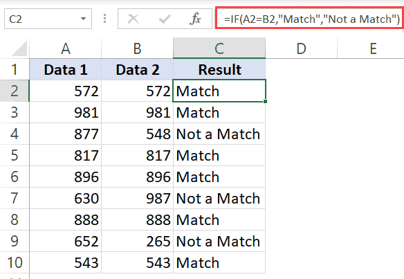
The above formula uses the same condition to check whether the two cells (in the same row) have matching data or not (A2=B2). But since we are using the IF function, we can ask it to return a specific text in case the condition is True or False.
Once you have the formula results in a separate column, you can quickly filter the data and get rows that have the matching data or rows with mismatched data.
Also read: Does Not Equal Operator in Excel (Examples)
Highlight Rows with Matching Data (or Different Data)
Another great way to quickly check the rows that have matching data (or have different data), is to highlight these rows using conditional formatting.
You can do both – highlight rows that have the same value in a row as well as the case when the value is different.
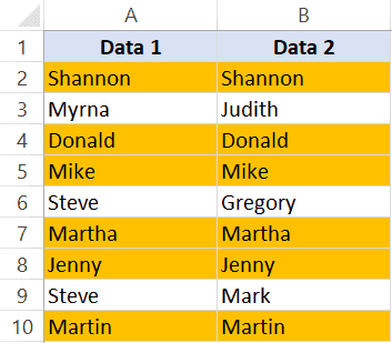
Suppose you have a dataset as shown below and you want to highlight all the rows where the name is the same.
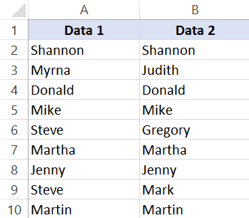
Below are the steps to use conditional formatting to highlight rows with matching data:
- Select the entire dataset (except the headers)
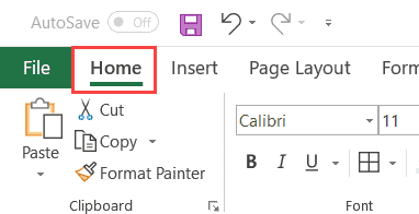
- Click the Home tab

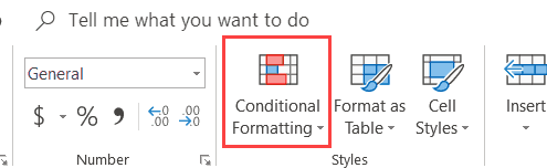
- In the Styles group, click on Conditional Formatting

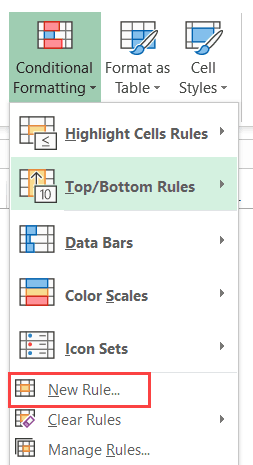
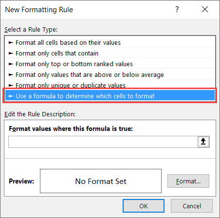
- In the options that show up, click on ‘New Rule’

- In the ‘New Formatting Rule’ dialog box, click on the option -”Use a formula to determine which cells to format’

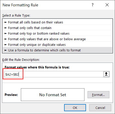
- In the ‘Format values where this formula is true’ field, enter the formula: =$A2=$B2
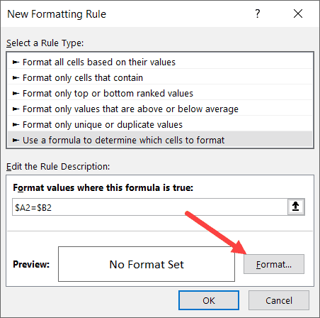
- Click on the Format button
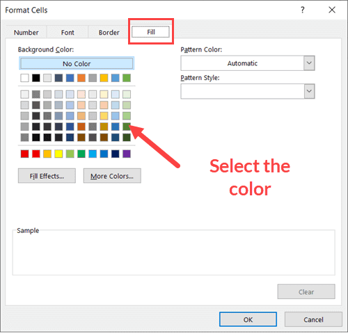
- Click on the ‘Fill’ tab and select the color in which you want to highlight the rows with the same value in both columns

- Click OK
The above steps would instantly highlight the rows where the name is the same in both columns A and B (in the same row). And in the case where the name is different, those rows will not be highlighted.
In case you want to compare two columns and highlight rows where the names are different, use the below formula in the conditional formatting dialog box (in step 6).
=$A2<>$B2
How does this work?
When we use conditional formatting with a formula, it only highlights those cells where the formula is true.
When we use $A2=$B2, it will check each cell (in both columns) and see whether the value in a row in column A is equal to the one in column B or not.
In case it’s an exact match, it will highlight it in the specified color, and in case it doesn’t match, it will not.
The best part about conditional formatting is that it doesn’t require you to use a formula in a separate column. Also, when you apply the rule on a dataset, it remains dynamic. This means that if you change any name in the dataset, conditional formatting will accordingly adjust.
Compare Two Columns Using VLOOKUP (Find Matching/Different Data)
In the above examples, I showed you how to compare two columns (or lists) when we are just comparing side by side cells.
In reality, this is rarely going to be the case.
In most cases, you will have two columns with data and you would have to find out whether a data point in one column exists in the other column or not.
In such cases, you can’t use a simple equal-to sign or even an IF function.
You need something more powerful…
… something that’s right up VLOOKUP’s alley!
Let me show you two examples where we compare two columns in Excel using the VLOOKUP function to find matches and differences.
Compare Two Columns Using VLOOKUP and Find Matches
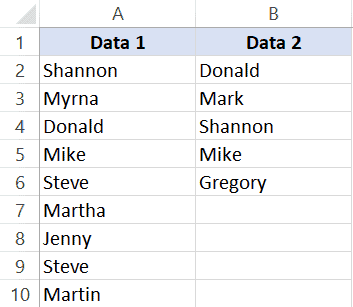
Suppose we have a dataset as shown below where we have some names in columns A and B.
If you have to find out what are the names that are in column B that are also in column A, you can use the below VLOOKUP formula:
=IFERROR(VLOOKUP(B2,$A$2:$A$10,1,0),"No Match")
The above formula compares the two columns (A and B) and gives you the name in case the name is in column B as well A, and it returns “No Match” in case the name is in Column B and not in Column A.
By default, the VLOOKUP function will return a #N/A error in case it doesn’t find an exact match. So to avoid getting the error, I have wrapped the VLOOKUP function in the IFERROR function, so that it gives “No Match” when the name is not available in column A.
You can also do the other way round comparison – to check whether the name is in Column A as well as Column B. The below formula would do that:
=IFERROR(VLOOKUP(A2,$B$2:$B$6,1,0),"No Match")
Compare Two Columns Using VLOOKUP and Find Differences (Missing Data Points)
While in the above example, we checked whether the data in one column was there in another column or not.
You can also use the same concept to compare two columns using the VLOOKUP function and find missing data.
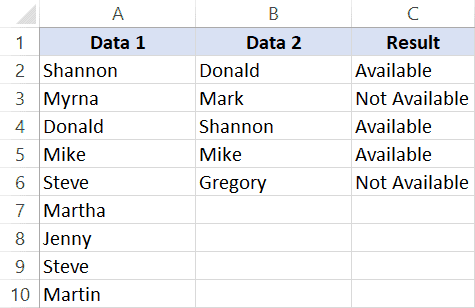
Suppose we have a dataset as shown below where we have some names in columns A and B.
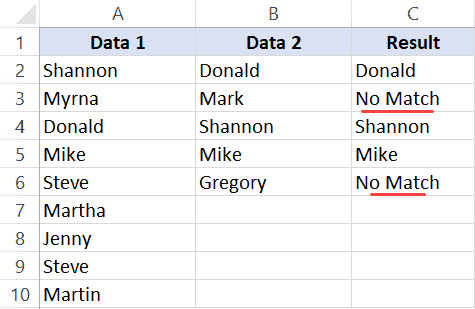
If you have to find out what are the names that are in column B that not there in column A, you can use the below VLOOKUP formula:
=IF(ISERROR(VLOOKUP(B2,$A$2:$A$10,1,0)),"Not Available","Available")
The above formula checks the name in column B against all the names in Column A. In case it finds an exact match, it would return that name, and in case it doesn’t find and exact match, it will return the #N/A error.
Since I am interested in finding the missing names that are there is column B and not in column A, I need to know the names that return the #N/A error.
This is why I have wrapped the VLOOKUP function in the IF and ISERROR functions. This whole formula gives the value – “Not Available” when the name is missing in Column A, and “Available” when it’s present.
To know all the names that are missing, you can filter the result column based on the “Not Available” value.
You can also use the below MATCH function to get the same result:
=IF(ISNUMBER(MATCH(B2,$A$2:$A$10,0)),"Available","Not Available")
Common Queries when Comparing Two Columns
Below are some common queries I usually get when people are trying to compare data in two columns in Excel.
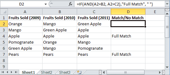
Q1. How to compare multiple columns in Excel in the same row for matches? Count the total duplicates also.
Ans. We have given the procedure to compare two columns in excel for the same row above. But if you want to compare multiple columns in excel for the same row then see the example
=IF(AND(A2=B2, A2=C2),"Full Match", "")
Here we have compared data of column A, column B, and column C. After this, I have applied the above formula in column D and get the result.
Now to count the duplicates, you need to use the Countif function.
=IF(COUNTIF($A2:$E2, $A2)=5, "Full Match", "")
Q2. Which operator do you use for matches and differences?
Ans. Below are the operators to use:
- To find matches, use the equal to sign (=)
- To find differences (mismatches), use the not-equal-to sign (<>)
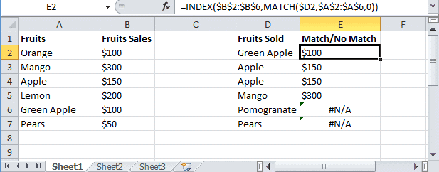
Q3. How to compare two different tables and pull matching data?
Ans. For this, you can use the VLOOKUP function or INDEX & MATCH function. To understand this thing in a better way we will take an example.
Here we will take two tables and now want to do pull matching data. In the first table, you have a dataset and in the second table, take the list of fruits and then use pull matching data in another column. For pull matching, use the formula
=INDEX($B$2:$B$6,MATCH($D2,$A$2:$A$6,0))
Q4. How to remove duplicates in Excel?
Ans. To remove duplicate data you need to first find the duplicate values.
To find the duplicate, you can use various methods like conditional formatting, Vlookup, If Statement, and many more. Excel also has an in-built tool where you can just select the data, and remove the duplicates from a column or even multiple columns
Q5. I can see that there is a matching value in both columns. However, the formulas you have shared above are not considering these as exact matches. Why?
Ans: Excel considers something an exact match when each and every character of one cell is equal to the other. There is a high chance that in your dataset there are leading or trailing spaces.
Although these spaces may still make the values seem equal to a naked eye, for Excel these are different. If you have such a dataset, it’s best to get rid of these spaces (you can use Excel functions such as TRIM for this).
Q7. How to compare two columns that give the result as TRUE when all first columns’ integer values are not less than the second column’s integer values. To solve this problem, I do not require conditional formatting, Vlookup function, If Statement, and any other formulas. I need the formula to solve this problem.
Ans. You can use the array formula for solving this problem.
The syntax is {=AND(H6:H12>I6:I12)}. This will give you “True” as a result whenever the value of Column H is greater than the value in column I else “False” will be the result.
You may also like the following Excel tutorials:
- Compare Two Columns in Excel (for matches and differences)
- How to Remove Blank Columns in Excel? (Formula + VBA)
- How to Hide Columns Based On Cell Value in Excel
- How to Split One Column into Multiple Columns in Excel
- How to Select Alternate Columns in Excel (or every Nth Column)
- How to Paste in a Filtered Column Skipping the Hidden Cells
- Best Excel Books (that will make you an Excel Pro)
- How to Flip Data in Excel (Columns, Rows, Tables)?
- Find the Closest Match in Excel (Nearest Value)
- How to Compare Two Cells in Excel?
- VLOOKUP Not Working – 7 Possible Reasons + How to Fix!
I was trying to compare A-B columns and highlight equal text, but usinng the obove fomrulas some text did not match at all. So I used form (VBA macro to compare two columns and color highlight cell differences) codes and I modified few things to adapt it to my application and find any desired column (just by clicking it). In my case, I use large and different numbers of rows on each column. Hope this helps:
Sub ABTextCompare()
Dim Report As Worksheet
Dim i, j, colNum, vMatch As Integer
Dim lastRowA, lastRowB, lastRow, lastColumn As Integer
Dim ColumnUsage As String
Dim colA, colB, colC As String
Dim A, B, C As Variant

Set Report = Excel.ActiveSheet
vMatch = 1

'Select A and B Columns to compare
On Error Resume Next
 Set A = Application.InputBox(Prompt:="Select column to compare", Title:="Column A", Type:=8)
  If A Is Nothing Then Exit Sub
colA = Split(A(1).Address(1, 0), "$")(0)
 Set B = Application.InputBox(Prompt:="Select column being searched", Title:="Column B", Type:=8)
   If A Is Nothing Then Exit Sub
  colB = Split(B(1).Address(1, 0), "$")(0)
 'Select Column to show results
 Set C = Application.InputBox("Select column  to show results", "Results", Type:=8)
    If C Is Nothing Then Exit Sub
  colC = Split(C(1).Address(1, 0), "$")(0)

'Get Last Row
lastRowA = Report.Cells.Find("", Range(colA & 1), xlFormulas, xlByRows, xlPrevious).Row - 1 ' Last row in column A
lastRowB = Report.Cells.Find("", Range(colB & 1), xlFormulas, xlByRows, xlPrevious).Row - 1 ' Last row in column B

 Application.ScreenUpdating = False
'***************************************************
For i = 2 To lastRowA
      For j = 2 To lastRowB
          If Report.Cells(i, A.Column).Value <> "" Then
              If InStr(1, Report.Cells(j, B.Column).Value, Report.Cells(i, A.Column).Value, vbTextCompare) > 0 Then
                  vMatch = vMatch + 1
                  Report.Cells(i, A.Column).Interior.ColorIndex = 35 'Light green background
                  Range(colC & 1).Value = "Items Found"
                  Report.Cells(i, A.Column).Copy Destination:=Range(colC & vMatch)
                  Exit For
              Else
                  'Do Nothing
              End If
          End If
      Next j
  Next i
If vMatch = 1 Then
    MsgBox Prompt:="No Itmes Found", Buttons:=vbInformation
End If
'***************************************************
Application.ScreenUpdating = True
End Sub
This post will guide you how to check if the values of multiple cells are equal with a formula in Excel. How do I verify that multiple cellsare the same in Excel. How to compare three or more cells in Excel to see if they are the same with a formula.
Table of Contents
- Check If Multiple Cells are Equal
- Related Functions
Assuming that you have a list of data in range A1:C1, and you want to compare if these cells are equal, if so, then return True, otherwise, return False. How to achieve it.
You need to create an Excel array formula based on the AND function and the EXACT function. Just like this:
=AND(EXACT(A1:C1,A1))
Type this formula into a blank cell, and press Ctrl +Shift +Enter shortcuts in your keyboard.
There is another formula based on the COUNTIF function to achieve the same result. Like this:
=COUNTIF(A1:C1,A1)=3
- Excel AND function
The Excel AND function returns TRUE if all of arguments are TRUE, and it returns FALSE if any of arguments are FALSE.The syntax of the AND function is as below:= AND (condition1,[condition2],…) … - Excel COUNTIF function
The Excel COUNTIF function will count the number of cells in a range that meet a given criteria. This function can be used to count the different kinds of cells with number, date, text values, blank, non-blanks, or containing specific characters.etc.= COUNTIF (range, criteria)… - Excel EXACT function
The Excel EXACT function compares if two text strings are the same and returns TRUE if they are the same, Or, it will return FALSE.The syntax of the EXACT function is as below:= EXACT (text1,text2)…