
The IF function allows you to make a logical comparison between a value and what you expect by testing for a condition and returning a result if that condition is True or False.
-
=IF(Something is True, then do something, otherwise do something else)
But what if you need to test multiple conditions, where let’s say all conditions need to be True or False (AND), or only one condition needs to be True or False (OR), or if you want to check if a condition does NOT meet your criteria? All 3 functions can be used on their own, but it’s much more common to see them paired with IF functions.
Use the IF function along with AND, OR and NOT to perform multiple evaluations if conditions are True or False.
Syntax
-
IF(AND()) — IF(AND(logical1, [logical2], …), value_if_true, [value_if_false]))
-
IF(OR()) — IF(OR(logical1, [logical2], …), value_if_true, [value_if_false]))
-
IF(NOT()) — IF(NOT(logical1), value_if_true, [value_if_false]))
|
Argument name |
Description |
|
|
logical_test (required) |
The condition you want to test. |
|
|
value_if_true (required) |
The value that you want returned if the result of logical_test is TRUE. |
|
|
value_if_false (optional) |
The value that you want returned if the result of logical_test is FALSE. |
|
Here are overviews of how to structure AND, OR and NOT functions individually. When you combine each one of them with an IF statement, they read like this:
-
AND – =IF(AND(Something is True, Something else is True), Value if True, Value if False)
-
OR – =IF(OR(Something is True, Something else is True), Value if True, Value if False)
-
NOT – =IF(NOT(Something is True), Value if True, Value if False)
Examples
Following are examples of some common nested IF(AND()), IF(OR()) and IF(NOT()) statements. The AND and OR functions can support up to 255 individual conditions, but it’s not good practice to use more than a few because complex, nested formulas can get very difficult to build, test and maintain. The NOT function only takes one condition.

Here are the formulas spelled out according to their logic:
|
Formula |
Description |
|---|---|
|
=IF(AND(A2>0,B2<100),TRUE, FALSE) |
IF A2 (25) is greater than 0, AND B2 (75) is less than 100, then return TRUE, otherwise return FALSE. In this case both conditions are true, so TRUE is returned. |
|
=IF(AND(A3=»Red»,B3=»Green»),TRUE,FALSE) |
If A3 (“Blue”) = “Red”, AND B3 (“Green”) equals “Green” then return TRUE, otherwise return FALSE. In this case only the first condition is true, so FALSE is returned. |
|
=IF(OR(A4>0,B4<50),TRUE, FALSE) |
IF A4 (25) is greater than 0, OR B4 (75) is less than 50, then return TRUE, otherwise return FALSE. In this case, only the first condition is TRUE, but since OR only requires one argument to be true the formula returns TRUE. |
|
=IF(OR(A5=»Red»,B5=»Green»),TRUE,FALSE) |
IF A5 (“Blue”) equals “Red”, OR B5 (“Green”) equals “Green” then return TRUE, otherwise return FALSE. In this case, the second argument is True, so the formula returns TRUE. |
|
=IF(NOT(A6>50),TRUE,FALSE) |
IF A6 (25) is NOT greater than 50, then return TRUE, otherwise return FALSE. In this case 25 is not greater than 50, so the formula returns TRUE. |
|
=IF(NOT(A7=»Red»),TRUE,FALSE) |
IF A7 (“Blue”) is NOT equal to “Red”, then return TRUE, otherwise return FALSE. |
Note that all of the examples have a closing parenthesis after their respective conditions are entered. The remaining True/False arguments are then left as part of the outer IF statement. You can also substitute Text or Numeric values for the TRUE/FALSE values to be returned in the examples.
Here are some examples of using AND, OR and NOT to evaluate dates.

Here are the formulas spelled out according to their logic:
|
Formula |
Description |
|---|---|
|
=IF(A2>B2,TRUE,FALSE) |
IF A2 is greater than B2, return TRUE, otherwise return FALSE. 03/12/14 is greater than 01/01/14, so the formula returns TRUE. |
|
=IF(AND(A3>B2,A3<C2),TRUE,FALSE) |
IF A3 is greater than B2 AND A3 is less than C2, return TRUE, otherwise return FALSE. In this case both arguments are true, so the formula returns TRUE. |
|
=IF(OR(A4>B2,A4<B2+60),TRUE,FALSE) |
IF A4 is greater than B2 OR A4 is less than B2 + 60, return TRUE, otherwise return FALSE. In this case the first argument is true, but the second is false. Since OR only needs one of the arguments to be true, the formula returns TRUE. If you use the Evaluate Formula Wizard from the Formula tab you’ll see how Excel evaluates the formula. |
|
=IF(NOT(A5>B2),TRUE,FALSE) |
IF A5 is not greater than B2, then return TRUE, otherwise return FALSE. In this case, A5 is greater than B2, so the formula returns FALSE. |

Using AND, OR and NOT with Conditional Formatting
You can also use AND, OR and NOT to set Conditional Formatting criteria with the formula option. When you do this you can omit the IF function and use AND, OR and NOT on their own.
From the Home tab, click Conditional Formatting > New Rule. Next, select the “Use a formula to determine which cells to format” option, enter your formula and apply the format of your choice.

Using the earlier Dates example, here is what the formulas would be.

|
Formula |
Description |
|---|---|
|
=A2>B2 |
If A2 is greater than B2, format the cell, otherwise do nothing. |
|
=AND(A3>B2,A3<C2) |
If A3 is greater than B2 AND A3 is less than C2, format the cell, otherwise do nothing. |
|
=OR(A4>B2,A4<B2+60) |
If A4 is greater than B2 OR A4 is less than B2 plus 60 (days), then format the cell, otherwise do nothing. |
|
=NOT(A5>B2) |
If A5 is NOT greater than B2, format the cell, otherwise do nothing. In this case A5 is greater than B2, so the result will return FALSE. If you were to change the formula to =NOT(B2>A5) it would return TRUE and the cell would be formatted. |
Note: A common error is to enter your formula into Conditional Formatting without the equals sign (=). If you do this you’ll see that the Conditional Formatting dialog will add the equals sign and quotes to the formula — =»OR(A4>B2,A4<B2+60)», so you’ll need to remove the quotes before the formula will respond properly.
Need more help?

See also
You can always ask an expert in the Excel Tech Community or get support in the Answers community.
Learn how to use nested functions in a formula
IF function
AND function
OR function
NOT function
Overview of formulas in Excel
How to avoid broken formulas
Detect errors in formulas
Keyboard shortcuts in Excel
Logical functions (reference)
Excel functions (alphabetical)
Excel functions (by category)
Excel has a number of formulas that help you use your data in useful ways. For example, you can get an output based on whether or not a cell meets certain specifications. Right now, we’ll focus on a function called “if cell contains, then”. Let’s look at an example.
Jump To Specific Section:
- Explanation: If Cell Contains
- If cell contains any value, then return a value
- If cell contains text/number, then return a value
- If cell contains specific text, then return a value
- If cell contains specific text, then return a value (case-sensitive)
- If cell does not contain specific text, then return a value
- If cell contains one of many text strings, then return a value
- If cell contains several of many text strings, then return a value
Excel Formula: If cell contains
Generic formula
=IF(ISNUMBER(SEARCH("abc",A1)),A1,"")
Summary
To test for cells that contain certain text, you can use a formula that uses the IF function together with the SEARCH and ISNUMBER functions. In the example shown, the formula in C5 is:
=IF(ISNUMBER(SEARCH("abc",B5)),B5,"")
If you want to check whether or not the A1 cell contains the text “Example”, you can run a formula that will output “Yes” or “No” in the B1 cell. There are a number of different ways you can put these formulas to use. At the time of writing, Excel is able to return the following variations:
- If cell contains any value
- If cell contains text
- If cell contains number
- If cell contains specific text
- If cell contains certain text string
- If cell contains one of many text strings
- If cell contains several strings
Using these scenarios, you’re able to check if a cell contains text, value, and more.
Explanation: If Cell Contains
One limitation of the IF function is that it does not support Excel wildcards like «?» and «*». This simply means you can’t use IF by itself to test for text that may appear anywhere in a cell.
One solution is a formula that uses the IF function together with the SEARCH and ISNUMBER functions. For example, if you have a list of email addresses, and want to extract those that contain «ABC», the formula to use is this:
=IF(ISNUMBER(SEARCH("abc",B5)),B5,""). Assuming cells run to B5
If «abc» is found anywhere in a cell B5, IF will return that value. If not, IF will return an empty string («»). This formula’s logical test is this bit:
ISNUMBER(SEARCH("abc",B5))
Read article: Excel efficiency: 11 Excel Formulas To Increase Your Productivity
Using “if cell contains” formulas in Excel
The guides below were written using the latest Microsoft Excel 2019 for Windows 10. Some steps may vary if you’re using a different version or platform. Contact our experts if you need any further assistance.
1. If cell contains any value, then return a value
This scenario allows you to return values based on whether or not a cell contains any value at all. For example, we’ll be checking whether or not the A1 cell is blank or not, and then return a value depending on the result.
- Select the output cell, and use the following formula: =IF(cell<>»», value_to_return, «»).
- For our example, the cell we want to check is A2, and the return value will be No. In this scenario, you’d change the formula to =IF(A2<>»», «No», «»).
- Since the A2 cell isn’t blank, the formula will return “No” in the output cell. If the cell you’re checking is blank, the output cell will also remain blank.
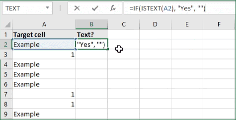
2. If cell contains text/number, then return a value
With the formula below, you can return a specific value if the target cell contains any text or number. The formula will ignore the opposite data types.
Check for text
- To check if a cell contains text, select the output cell, and use the following formula: =IF(ISTEXT(cell), value_to_return, «»).
- For our example, the cell we want to check is A2, and the return value will be Yes. In this scenario, you’d change the formula to =IF(ISTEXT(A2), «Yes», «»).

- Because the A2 cell does contain text and not a number or date, the formula will return “Yes” into the output cell.
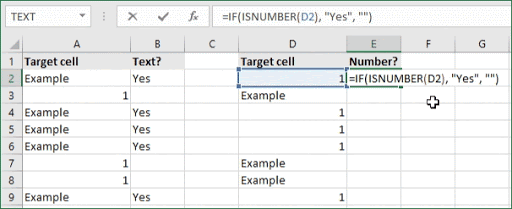
Check for a number or date
- To check if a cell contains a number or date, select the output cell, and use the following formula: =IF(ISNUMBER(cell), value_to_return, «»).
- For our example, the cell we want to check is D2, and the return value will be Yes. In this scenario, you’d change the formula to =IF(ISNUMBER(D2), «Yes», «»).

- Because the D2 cell does contain a number and not text, the formula will return “Yes” into the output cell.
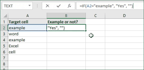
3. If cell contains specific text, then return a value
To find a cell that contains specific text, use the formula below.
- Select the output cell, and use the following formula: =IF(cell=»text», value_to_return, «»).
- For our example, the cell we want to check is A2, the text we’re looking for is “example”, and the return value will be Yes. In this scenario, you’d change the formula to =IF(A2=»example», «Yes», «»).

- Because the A2 cell does consist of the text “example”, the formula will return “Yes” into the output cell.
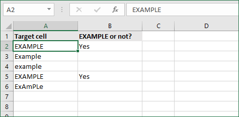
4. If cell contains specific text, then return a value (case-sensitive)
To find a cell that contains specific text, use the formula below. This version is case-sensitive, meaning that only cells with an exact match will return the specified value.
- Select the output cell, and use the following formula: =IF(EXACT(cell,»case_sensitive_text»), «value_to_return», «»).
- For our example, the cell we want to check is A2, the text we’re looking for is “EXAMPLE”, and the return value will be Yes. In this scenario, you’d change the formula to =IF(EXACT(A2,»EXAMPLE»), «Yes», «»).
- Because the A2 cell does consist of the text “EXAMPLE” with the matching case, the formula will return “Yes” into the output cell.
5. If cell does not contain specific text, then return a value
The opposite version of the previous section. If you want to find cells that don’t contain a specific text, use this formula.
- Select the output cell, and use the following formula: =IF(cell=»text», «», «value_to_return»).
- For our example, the cell we want to check is A2, the text we’re looking for is “example”, and the return value will be No. In this scenario, you’d change the formula to =IF(A2=»example», «», «No»).
- Because the A2 cell does consist of the text “example”, the formula will return a blank cell. On the other hand, other cells return “No” into the output cell.
6. If cell contains one of many text strings, then return a value
This formula should be used if you’re looking to identify cells that contain at least one of many words you’re searching for.
- Select the output cell, and use the following formula: =IF(OR(ISNUMBER(SEARCH(«string1», cell)), ISNUMBER(SEARCH(«string2», cell))), value_to_return, «»).
- For our example, the cell we want to check is A2. We’re looking for either “tshirt” or “hoodie”, and the return value will be Valid. In this scenario, you’d change the formula to =IF(OR(ISNUMBER(SEARCH(«tshirt»,A2)),ISNUMBER(SEARCH(«hoodie»,A2))),»Valid «,»»).
- Because the A2 cell does contain one of the text values we searched for, the formula will return “Valid” into the output cell.
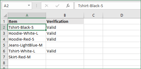
To extend the formula to more search terms, simply modify it by adding more strings using ISNUMBER(SEARCH(«string», cell)).
7. If cell contains several of many text strings, then return a value
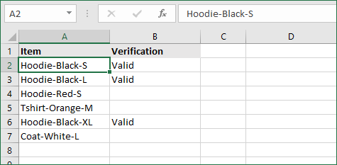
This formula should be used if you’re looking to identify cells that contain several of the many words you’re searching for. For example, if you’re searching for two terms, the cell needs to contain both of them in order to be validated.
- Select the output cell, and use the following formula: =IF(AND(ISNUMBER(SEARCH(«string1»,cell)), ISNUMBER(SEARCH(«string2″,cell))), value_to_return,»»).
- For our example, the cell we want to check is A2. We’re looking for “hoodie” and “black”, and the return value will be Valid. In this scenario, you’d change the formula to =IF(AND(ISNUMBER(SEARCH(«hoodie»,A2)),ISNUMBER(SEARCH(«black»,A2))),»Valid «,»»).
- Because the A2 cell does contain both of the text values we searched for, the formula will return “Valid” to the output cell.
Final thoughts
We hope this article was useful to you in learning how to use “if cell contains” formulas in Microsoft Excel. Now, you can check if any cells contain values, text, numbers, and more. This allows you to navigate, manipulate and analyze your data efficiently.
We’re glad you’re read the article up to here  Thank you
You may also like
» How to use NPER Function in Excel
» How to Separate First and Last Name in Excel
» How to Calculate Break-Even Analysis in Excel
Tests if a given value is a text string or not
What is the ISTEXT Function?
The ISTEXT Function[1] is categorized under Excel Information functions. The function will test if a given value is a text string or not. If the given value is text, it will return TRUE, or if not, it will return FALSE.
In doing financial analysis, if we want a particular file to input only text values in a designated cell, using this function along with data validation will help us do that.
Formula
=ISTEXT(value)
The ISTEXT function uses only one argument:
- Value (required argument) – This is the given value or expression that we wish to test. The value argument can be a blank (i.e., an empty cell), an error, a logical value, a text, a number, a reference value, or a name referring to any of these.
How to use the ISTEXT Function in Excel?
As a worksheet function, ISTEXT can be entered as part of a formula in a cell of a worksheet.
To understand the uses of the ISTEXT function, let’s consider a few examples:
Example 1
Suppose we are given the following data:
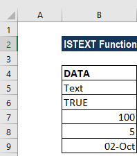
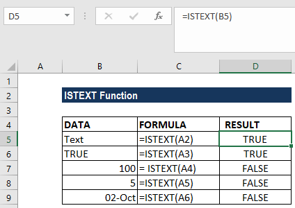
As we see above, when we apply the ISTEXT formula, we get the result in the form of TRUE or FALSE.
Example 2
Suppose we wish to allow only text to be entered in a particular cell. In such a scenario, we can use data validation along with ISTEXT to get the desired results.
Using the data below:
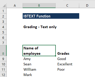
We want only text to be entered in column C9:C12, so we apply data validation to the cells. The formula to be used would be =ISTEXT(B9).
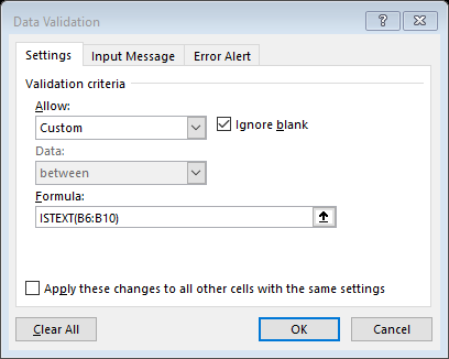
How to apply this formula?
We need to go to the Data tab. Under the Data tab, click on Data Validation, then click on Validation criteria and select “Custom”. Use a formula to determine which cells to format. For this example, we selected column B6:B10:
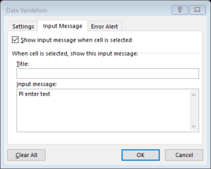
If we want, we can input an error message. Click on Input Message and type the message on the Input message box.
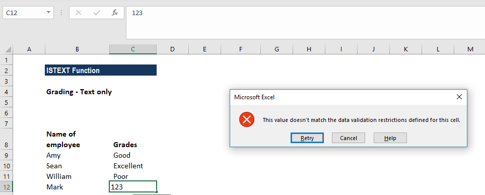
Now, click OK.
Data validation rules are now triggered when any user adds or changes a cell value. Cell references in data validation formulas are checked for rules defined in data validation.
The ISTEXT function returns TRUE when a value is text and FALSE if it is not. As a result, all text input will pass validation, but numbers and formulas will fail validation.
We get the results below when we try to enter numbers:
Example 3
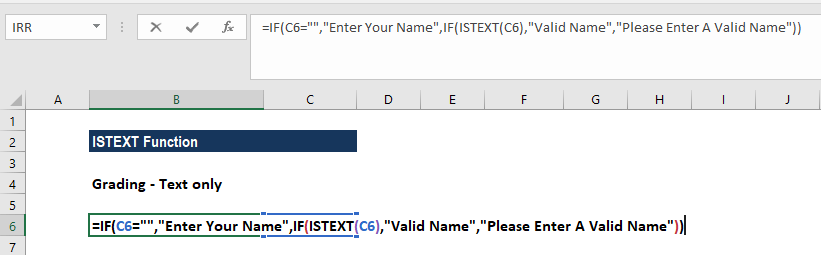
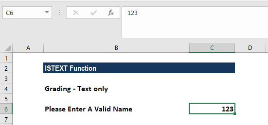
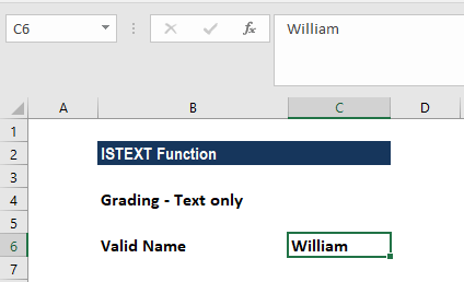
We can also ensure valid text is entered by using ISTEXT with the IF function. This can be done using a nesting formula. Suppose we have a form that is to be filled out by users. The form is being sent to various users. We want to ensure that only names are entered in cell B3. For this, we will use the formula =IF(B3=””,”Enter Your Name”,IF(ISTEXT(B3),”Valid Name”,”Please Enter A Valid Name”)), as shown below:
If we try to input a number, we will get an error, while a valid name will be accepted, as shown below.
A few things to remember about the ISTEXT Function
- The ISTEXT function is available in MS Excel 2000 and later versions.
- The function will return FALSE even for formula errors such as #VALUE!, #NULL!, etc.
- ISTEXT belongs to the IS family. We can use an IS function to get information about a value before performing a calculation or other action on it.
Click here to download the sample Excel file
Additional Resources
Thanks for reading CFI’s guide to important Excel functions! By taking the time to learn and master these functions, you’ll significantly speed up your financial analysis. To learn more, check out these additional CFI resources:
- Excel Finance Functions
- Advanced Excel Formulas Course
- Advanced Excel Formulas to Know
- Excel Keyboard Shortcuts
- See all Excel resources
Article Sources
- ISTEXT Function
Normally, If you want to write an IF formula for text values in combining with the below two logical operators in excel, such as: “equal to” or “not equal to”.
Table of Contents
- Excel IF function check if a cell contains text(case-insensitive)
- Excel IF function check if a cell contains text (case-sensitive)
- Excel IF function check if part of cell matches specific text
- Excel IF function with Wildcards text value
- Related Formulas
- Related Functions
Excel IF function check if a cell contains text(case-insensitive)
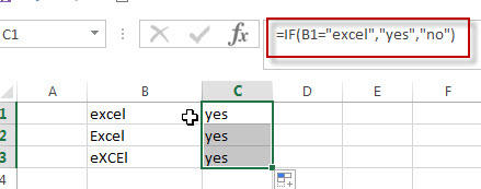
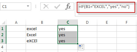
By default, IF function is case-insensitive in excel. It means that the logical text for text values will do not recognize case in the IF formulas. For example, the following two IF formulas will get the same results when checking the text values in cells.
=IF(B1="excel","yes","no")
=IF(B1="EXCEl","yes","no")
The IF formula will check the values of cell B1 if it is equal to “excel” word, If it is TRUE, then return “yes”, otherwise return “no”. And the logical test in the above IF formula will check the text values in the logical_test argument, whatever the logical_test values are “Excel”, “eXcel”, or “EXCEL”, the IF formula don’t care about that if the text values is in lowercase or uppercase, It will get the same results at last.
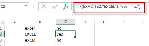
Excel IF function check if a cell contains text (case-sensitive)
If you want to check text values in cells using IF formula in excel (case-sensitive), then you need to create a case-sensitive logical test and then you can use IF function in combination with EXACT function to compare two text values. So if those two text values are exactly the same, then return TRUE. Otherwise return FALSE.
So we can write down the following IF formula combining with EXACT function:
=IF(EXACT(B1,"excel"),"yes","no")
Excel IF function check if part of cell matches specific text
If you want to check if part of text values in cell matches the specific text rather than exact match, to achieve this logic text, you can use IF function in combination with ISNUMBER and SEARCH Function in excel.
Both ISNUMBER and SEARCH functions are case-insensitive in excel.
=IF(ISNUMBER(SEARCH("x",B1)),"good","bad")
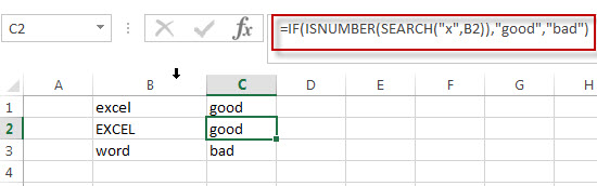
For above the IF formula, it will Check to see if B1 contain the letter x.
Also, we can use FIND function to replace the SEARCH function in the above IF formula. It will return the same results.
Excel IF function with Wildcards text value
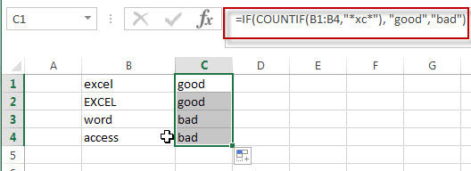
If you wan to use wildcard charcter in an IF formula, for example, if any of the values in column B contains “*xc*”, then return “good”, others return “bad”. You can not directly use the wildcard characters in IF formula, and we can use IF function in combination with COUNTIF function. Let’s see the following IF formula:
=IF(COUNTIF(B1:B4,"*xc*"), "good","bad")
- Excel IF Function With Numbers
If you want to check if a cell values is between two values or checking for the range of numbers or multiple values in cells, at this time, we need to use AND or OR logical function in combination with the logical operator and IF function…
- Excel EXACT function
The Excel SEARCH function returns the number of the starting location of a substring in a text string.The syntax of the EXACT function is as below:= EXACT (text1,text2)… - Excel COUNTIF function
The Excel COUNTIF function will count the number of cells in a range that meet a given criteria.= COUNTIF (range, criteria) … - Excel ISNUMBER function
The Excel ISNUMBER function returns TRUE if the value in a cell is a numeric value, otherwise it will return FALSE. - Excel IF function
The Excel IF function perform a logical test to return one value if the condition is TRUE and return another value if the condition is FALSE…. - Excel SEARCH function
The Excel SEARCH function returns the number of the starting location of a substring in a text string.…
Purpose
Test for a non-text value
Return value
A logical value (TRUE or FALSE)
Usage notes
The ISNONTEXT function returns TRUE when a cell contains any value except text. This includes numbers, dates, times, errors, and formulas that return non-text results. ISNONTEXT also returns TRUE when a cell is empty.
The ISNONTEXT function takes one argument, value, which can be a cell reference, a formula, or a hardcoded value. Typically, value is entered as a cell reference like A1. When value is not text, the ISNONTEXT function will return TRUE. If value is text, ISNONTEXT will return FALSE.
Examples
The ISNONTEXT function returns TRUE for numbers and FALSE for text:
=ISNONTEXT(100) // returns TRUE
=ISNONTEXT("apple") // returns FALSE
If cell A1 contains the number 100, ISNONTEXT returns TRUE:
=ISNONTEXT(A1) // returns TRUE
If cell A1 is empty, ISNONTEXT returns TRUE:
=ISNONTEXT(A1) // returns TRUE
If a cell contains a formula, ISNONTEXT checks the result of the formula:
=ISNONTEXT(2+2) // returns TRUE
=ISNONTEXT(10 &" apples") // returns FALSE
=ISNONTEXT(A1&B1) // returns FALSE
Note: the ampersand (&) is the concatenation operator in Excel. When values are concatenated, the result is text.
Count text non values
To count cells in a range that do not contain text with the ISNONTEXT function, you can use the SUMPRODUCT function like this:
=SUMPRODUCT(--ISNONTEXT(range))
The double negative coerces the TRUE and FALSE results from ISNONTEXT into 1s and 0s and SUMPRODUCT sums the result. You can also use the COUNTIF function to count cells that do not contain text, as explained here.
Notes
- When value is a number, ISNONTEXT returns TRUE.
- When value is any error, ISNONTEXT returns TRUE.
- When value is an empty cell, ISNONTEXT returns TRUE.
EXPLANATION
This tutorial shows how to test if a cell contains text and return a specified value if the test is True or False by using Excel formulas or VBA.
This tutorial provides three Excel methods that can be applied to test if a cell contains text.
The first method uses a combination of an Excel IF and ISTEXT functions. The ISTEXT function test if the selected cell contains text. If it does then the function will return a TRUE value. The IF function is then used to return a specified value if the ISTEXT function returns a value of TRUE, which in this example is «Contains Text». Alternatively, if the ISTEXT function returns a value of FALSE, then the cell does not contain text and the IF function will return the associated value, which in this example is «No Text».
The second method uses a combination of an Excel IF and ISNUMBER functions. The ISNUMBER function test if the selected cell is a numeric value. If the cell is a numeric value, meaning that there are no text values, then the function will return a TRUE value, alternatively if the cell contains a text value, the function will return a FALSE value. The IF function is then used to return a specified value if the ISNUMBER function returns a value of FALSE, which in this example is «Contains Text». Alternatively, if the ISNUMBER function returns a value of TRUE, then the cell does not contain text and the IF function will return the associated value, which in this example is «No Text».
The third method uses a combination of an Excel IF and COUNTIF functions. The COUNTIF function uses the «*» to identify if the cell contains text. If the cell contains text the COUNTIF function will return a value of 1, alternatively it will return a value of 0. The IF function is then used to return a specified value if the COUNTIF function returns a value greater than 0, which in this example is «Contains Text». Alternatively, if the COUNTIF function returns a value of 0, then the cell does not contain text and the IF function will return the associated value, which in this example is «No Text».
This tutorial provides six VBA methods that can be applied to test if a cell contains text and return a specific value. Methods 1, 3 and 5 are applied against a single cell, whilst methods 2, 4 and 6 use a For Loop to loop through all of the relevant cells, as per the example in the image, to test each of the cells in a range and return specific values. The main difference between the examples is how the code determines is the cell contains text.
FORMULA (using ISTEXT function)
=IF(ISTEXT(value)=TRUE, value_if_true, value_if_false)
FORMULA (using ISNUMBER function)
=IF(ISNUMBER(value)=FALSE, value_if_true, value_if_false)
FORMULA (using COUNTIF function)
=IF(COUNTIF(value, «*»)>0, value_if_true, value_if_false)
ARGUMENTS
value: The value or cell that is to be tested.
value_if_true: Value to be returned if the value or cell contains text.
value_if_false: Value to be returned if the value or cell does not contains text.
The logical IF statement in Excel is used for the recording of certain conditions. It compares the number and / or text, function, etc. of the formula when the values correspond to the set parameters, and then there is one record, when do not respond — another.
Logic functions — it is a very simple and effective tool that is often used in practice. Let us consider it in details by examples.
The syntax of the function «IF» with one condition
The operation syntax in Excel is the structure of the functions necessary for its operation data.
=IF(boolean;value_if_TRUE;value_if_FALSE)
Let us consider the function syntax:
- Boolean – what the operator checks (text or numeric data cell).
- Value_if_TRUE – what will appear in the cell when the text or numbers correspond to a predetermined condition (true).
- Value_if_FALSE – what appears in the box when the text or the number does not meet the predetermined condition (false).
Example:

Logical IF functions.
The operator checks the A1 cell and compares it to 20. This is a «Boolean». When the contents of the column is more than 20, there is a true legend «greater 20». In the other case it’s «less or equal 20».
Attention! The words in the formula need to be quoted. For Excel to understand that you want to display text values.
Here is one more example. To gain admission to the exam, a group of students must successfully pass a test. The results are listed in a table with columns: a list of students, a credit, an exam.

The statement IF should check not the digital data type but the text. Therefore, we prescribed in the formula В2= «done» We take the quotes for the program to recognize the text correctly.
The function IF in Excel with multiple conditions
Usually one condition for the logic function is not enough. If you need to consider several options for decision-making, spread operators’ IF into each other. Thus, we get several functions IF in Excel.
The syntax is as follows:
Here the operator checks the two parameters. If the first condition is true, the formula returns the first argument is the truth. False — the operator checks the second condition.
Examples of a few conditions of the function IF in Excel:

It’s a table for the analysis of the progress. The student received 5 points:
- А – excellent;
- В – above average or superior work;
- C – satisfactory;
- D – a passing grade;
- E – completely unsatisfactory.
IF statement checks two conditions: the equality of value in the cells.

In this example, we have added a third condition, which implies the presence of another report card and «twos». The principle of the operator is the same.
Enhanced functionality with the help of the operators «AND» and «OR»
When you need to check out a few of the true conditions you use the function И. The point is: IF A = 1 AND A = 2 THEN meaning в ELSE meaning с.
OR function checks the condition 1 or condition 2. As soon as at least one condition is true, the result is true. The point is: IF A = 1 OR A = 2 THEN value B ELSE value C.
Functions AND & OR can check up to 30 conditions.
An example of using the operator AND:

It’s the example of using the logical operator OR.

How to compare data in two tables
Users often need to compare the two spreadsheets in an Excel to match. Examples of the «life»: compare the prices of goods in different bringing, to compare balances (accounting reports) in a few months, the progress of pupils (students) of different classes, in different quarters, etc.
To compare the two tables in Excel, you can use the COUNTIFS statement. Consider the order of application functions.
For example, consider the two tables with the specifications of various food processors. We planned allocation of color differences. This problem in Excel solves the conditional formatting.
Baseline data (tables, which will work with):

Select the first table. Conditional Formatting — create a rule — use a formula to determine the formatted cells:

In the formula bar write: = COUNTIFS (comparable range; first cell of first table)=0. Comparing range is in the second table.
To drive the formula into the range, just select it first cell and the last. «= 0» means the search for the exact command (not approximate) values.
Choose the format and establish what changes in the cell formula in compliance. It’s better to do a color fill.
Select the second table. Conditional Formatting — create a rule — use the formula. Use the same operator (COUNTIFS). For the second table formula:
Download all examples in Excel

Now it is easy to compare the characteristics of the data in the table.