Excel if value is not a function - Word и Excel - помощь в работе с программами

IF function

The IF function is one of the most popular functions in Excel, and it allows you to make logical comparisons between a value and what you expect.

So an IF statement can have two results. The first result is if your comparison is True, the second if your comparison is False.

For example, =IF(C2=”Yes”,1,2) says IF(C2 = Yes, then return a 1, otherwise return a 2).

Use the IF function, one of the logical functions, to return one value if a condition is true and another value if it’s false.

IF(logical_test, value_if_true, [value_if_false])

For example:

=IF(A2>B2,»Over Budget»,»OK»)
=IF(A2=B2,B4-A4,»»)

Argument name	Description
logical_test (required)	The condition you want to test.
value_if_true (required)	The value that you want returned if the result of *logical_test* is TRUE.
value_if_false (optional)	The value that you want returned if the result of *logical_test* is FALSE.

Simple IF examples

=IF(C2=”Yes”,1,2)

In the above example, cell D2 says: IF(C2 = Yes, then return a 1, otherwise return a 2)

=IF(C2=1,”Yes”,”No”)

In this example, the formula in cell D2 says: IF(C2 = 1, then return Yes, otherwise return No)As you see, the IF function can be used to evaluate both text and values. It can also be used to evaluate errors. You are not limited to only checking if one thing is equal to another and returning a single result, you can also use mathematical operators and perform additional calculations depending on your criteria. You can also nest multiple IF functions together in order to perform multiple comparisons.

=IF(C2>B2,”Over Budget”,”Within Budget”)

In the above example, the IF function in D2 is saying IF(C2 Is Greater Than B2, then return “Over Budget”, otherwise return “Within Budget”)

=IF(C2>B2,C2-B2,0)

In the above illustration, instead of returning a text result, we are going to return a mathematical calculation. So the formula in E2 is saying IF(Actual is Greater than Budgeted, then Subtract the Budgeted amount from the Actual amount, otherwise return nothing).

=IF(E7=”Yes”,F5*0.0825,0)

In this example, the formula in F7 is saying IF(E7 = “Yes”, then calculate the Total Amount in F5 * 8.25%, otherwise no Sales Tax is due so return 0)

Note: If you are going to use text in formulas, you need to wrap the text in quotes (e.g. “Text”). The only exception to that is using TRUE or FALSE, which Excel automatically understands.

Common problems

Problem	What went wrong
0 (zero) in cell	There was no argument for either value_if_true or value_if_False arguments. To see the right value returned, add argument text to the two arguments, or add TRUE or FALSE to the argument.
#NAME? in cell	This usually means that the formula is misspelled.

Need more help?

You can always ask an expert in the Excel Tech Community or get support in the Answers community.

What is a Logical Function?

It is a feature that allows us to introduce decision-making when executing formulas and functions. Functions are used to;

Check if a condition is true or false
Combine multiple conditions together

What is a condition and why does it matter?

A condition is an expression that either evaluates to true or false. The expression could be a function that determines if the value entered in a cell is of numeric or text data type, if a value is greater than, equal to or less than a specified value, etc.

IF Function example

We will work with the home supplies budget from this tutorial. We will use the IF function to determine if an item is expensive or not. We will assume that items with a value greater than 6,000 are expensive. Those that are less than 6,000 are less expensive. The following image shows us the dataset that we will work with.

Put the cursor focus in cell F4
Enter the following formula that uses the IF function

=IF(E4<6000,”Yes”,”No”)

HERE,

“=IF(…)” calls the IF functions
“E4<6000” is the condition that the IF function evaluates. It checks the value of cell address E4 (subtotal) is less than 6,000
“Yes” this is the value that the function will display if the value of E4 is less than 6,000
“No” this is the value that the function will display if the value of E4 is greater than 6,000

When you are done press the enter key

You will get the following results

Excel Logic functions explained

The following table shows all of the logical functions in Excel

S/N	FUNCTION	CATEGORY	DESCRIPTION	USAGE
01	AND	Logical	Checks multiple conditions and returns true if they all the conditions evaluate to true.	=AND(1 > 0,ISNUMBER(1)) The above function returns TRUE because both Condition is True.
02	FALSE	Logical	Returns the logical value FALSE. It is used to compare the results of a condition or function that either returns true or false	FALSE()
03	IF	Logical	Verifies whether a condition is met or not. If the condition is met, it returns true. If the condition is not met, it returns false. =IF(logical_test,[value_if_true],[value_if_false])	=IF(ISNUMBER(22),”Yes”, “No”) 22 is Number so that it return Yes.
04	IFERROR	Logical	Returns the expression value if no error occurs. If an error occurs, it returns the error value	=IFERROR(5/0,”Divide by zero error”)
05	IFNA	Logical	Returns value if #N/A error does not occur. If #N/A error occurs, it returns NA value. #N/A error means a value if not available to a formula or function.	=IFNA(D6*E6,0) N.B the above formula returns zero if both or either D6 or E6 is/are empty
06	NOT	Logical	Returns true if the condition is false and returns false if condition is true	=NOT(ISTEXT(0)) N.B. the above function returns true. This is because ISTEXT(0) returns false and NOT function converts false to TRUE
07	OR	Logical	Used when evaluating multiple conditions. Returns true if any or all of the conditions are true. Returns false if all of the conditions are false	=OR(D8=”admin”,E8=”cashier”) N.B. the above function returns true if either or both D8 and E8 admin or cashier
08	TRUE	Logical	Returns the logical value TRUE. It is used to compare the results of a condition or function that either returns true or false	TRUE()

A nested IF function is an IF function within another IF function. Nested if statements come in handy when we have to work with more than two conditions. Let’s say we want to develop a simple program that checks the day of the week. If the day is Saturday we want to display “party well”, if it’s Sunday we want to display “time to rest”, and if it’s any day from Monday to Friday we want to display, remember to complete your to do list.

A nested if function can help us to implement the above example. The following flowchart shows how the nested IF function will be implemented.

The formula for the above flowchart is as follows

=IF(B1=”Sunday”,”time to rest”,IF(B1=”Saturday”,”party well”,”to do list”))

HERE,

“=IF(….)” is the main if function
“=IF(…,IF(….))” the second IF function is the nested one. It provides further evaluation if the main IF function returned false.

Practical example

Create a new workbook and enter the data as shown below

Enter the following formula

=IF(B1=”Sunday”,”time to rest”,IF(B1=”Saturday”,”party well”,”to do list”))

Enter Saturday in cell address B1
You will get the following results

Download the Excel file used in Tutorial

Summary

Logical functions are used to introduce decision-making when evaluating formulas and functions in Excel.

Источник

What is IF Function in Excel?

IF function in Excel evaluates whether a given condition is met and returns a value depending on whether the result is “true” or “false”. It is a conditional function of Excel, which returns the result based on the fulfillment or non-fulfillment of the given criteria.

For example, the IF formula in Excel can be applied as follows:

“=IF(condition A,“value B”,“value C”)”

The IF excel function returns “value B” if condition A is met and returns “value C” if condition A is not met.

It is often used to make logical interpretations which help in decision-making.

What is IF Function in Excel?
- Syntax of the IF Excel Function
- How to Use IF Function in Excel?
  - Example #1
  - Example #2
  - Example #3
  - Example #4
  - Example #5
- Guidelines for the Multiple IF Statements
- Frequently Asked Question
- IF Excel Function Video
- Recommended Articles

Syntax of the IF Excel Function

The syntax of the IF function is shown in the following image:

The IF excel function accepts the following arguments:

Logical_test: It refers to the condition to be evaluated. The condition can be a value or a logical expression.
Value_if_true: It is the value returned as a result when the condition is “true”.
Value_if_false: It is the value returned as a result when the condition is “false”.

In the formula, the “logical_test” is a required argument, whereas the “value_if_true” and “value_if_false” are optional arguments.

The IF formula uses logical operators to evaluate the values in a range of cells. The following table shows the different logical operatorsLogical operators in excel are also known as the comparison operators and they are used to compare two or more values, the return output given by these operators are either true or false, we get true value when the conditions match the criteria and false as a result when the conditions do not match the criteria.read more and their meaning.

Operator	Meaning
=	Equal to
>	Greater than
>=	Greater than or equal to
<	Less than
<=	Less than or equal to
<>	Not equal to

How to Use IF Function in Excel?

Let us understand the working of the IF function with the help of the following examples in Excel.

You can download this IF Function Excel Template here – IF Function Excel Template

Example #1

If there is no oxygen on a planet, life is impossible. If oxygen is available on a planet, then life is possible. The following table shows a list of planets in column A and the information on the availability of oxygen in column B. We have to find the planets where life is possible, based on the condition of oxygen availability.

Let us apply the IF formula to cell C2 to find out whether life is possible on the planets listed in the table.

The IF formula is stated as follows:

“=IF(B2=“Yes”, “Life is Possible”, “Life is Not Possible”)

The succeeding image shows the IF formula applied to cell C2.

The subsequent image shows how the IF formula is applied to the range of cells C2:C5.

Drag the cells to view the output of all the planets.

The output in the below worksheet shows life is possible on the planet Earth.

Flow Chart of Generic IF Excel Function

The IF Function Flow Chart for Mars (Example #1)

The flow of IF function flowchart for Jupiter and Venus is the same as the IF function flowchart for Mars (Example #1).

The IF Function Flow Chart for Earth

Hence, the IF excel function allows making logical comparisons between values. The modus operandi of the IF function is stated as: If something is true, then do something; otherwise, do something else.

Example #2

The following table shows a list of years. We want to find out if the given year is a leap year or not.

A leap year has 366 days; the extra day is the 29th of February. The criteria for a leap year are stated as follows:

The year will be exactly divisible by 4 and not exactly be divisible by 100 or
The year will be exactly divisible by 400.

In this example, we will use the IF function along with the AND, OR, and MOD functions to find the leap years.

We use the MOD function to find a remainder after a dividend is divided by a divisor.

The AND functionThe AND function in Excel is classified as a logical function; it returns TRUE if the specified conditions are met, otherwise it returns FALSE.read more evaluates both the conditions of the leap years for the value “true”. The OR functionThe OR function in Excel is used to test various conditions, allowing you to compare two values or statements in Excel. If at least one of the arguments or conditions evaluates to TRUE, it will return TRUE. Similarly, if all of the arguments or conditions are FALSE, it will return FASLE.read more evaluates either of the condition for the value “true”.

We will apply the MOD function to the conditions as follows:

If MOD(year,4)=0 and MOD(year,100)<>(is not equal to) 0, then the year is a leap year.

If MOD(year,400)=0, then the year is a leap year; otherwise, the year is not a leap year.

The IF formula is stated as follows:

“=IF(OR(AND((MOD(year,4)=0),(MOD(year,100)<>0)),(MOD(year,400)=0)),“Leap Year”, “Not A Leap Year”)”

The argument “year” refers to a reference value.

The following images show the output of the IF formula applied in the range of cells.

The following image shows how the IF formula is applied to the range of cells B2:B18.

The succeeding table shows the years 1960, 2028, and 2148 as leap years and the remaining as non-leap years.

The result of the IF excel formula is displayed for the range of cells B2:B18 in the following image.

Example #3

The succeeding table shows a list of drivers and the directions they undertook to reach the destination. It is preceded by an image of the road intersection explaining the turns taken by the drivers and their destinations. The right turn leads to town B, and the left turn leads to town C. Identify the driver’s destination to town B and town C.

Road Intersection Image

Let us apply the IF excel function to find the destination. Here, the condition is mentioned as follows:

If the driver turns right, he/she reaches town B.
If the driver turns left, he/she reaches town C.

We use the following IF formula to find the destination:

“=IF(B2=“Left”, “Town C”, “Town B”)”

The succeeding image shows the output of the IF formula applied to cell C2.

Drag the cells to use the formula in the range C2:C11. Finally, we get the destinations of each driver for their turning movements.

The below image displays the IF formula applied to the range.

The output of the IF formula and the destinations are displayed in the succeeding image.

The result shows that six drivers reached town C, and the remaining four have reached town B.

Example #4

The following table shows a list of items and their inventory levels. We want to check if the specific item is available in the inventory or not using the IF function.

Let us list the name of items in column A and the number of items in column B. The list of data to be validated for the entire items list is shown in the cell E2 of the below image.

We use the Excel IF along with the VLOOKUP functionThe VLOOKUP excel function searches for a particular value and returns a corresponding match based on a unique identifier. A unique identifier is uniquely associated with all the records of the database. For instance, employee ID, student roll number, customer contact number, seller email address, etc., are unique identifiers.
read more to check the availability of the items in the inventory.

The VLOOKUP function looks up the values referring to the number of items, and the IF function will check whether the item number is greater than zero or not.

We will apply the following IF formula in the F2 cell:

“=IF(VLOOKUP(E2,A2:B11,2,0)=0, “Item Not Available”,“Item Available”)”

If the lookup value of an item is equal to 0, then the item is not available; else, the item is available.

The succeeding image shows the result of the IF formula in the cell F2.

Select “bat” in the E2 item cell to know whether the item is available or not in the inventory (as shown in the following image).

Example #5

The following table shows the list of students and their marks. The grade criteria are provided based on the marks obtained by the students. We want to find the grade of each student in the list.

We apply the Nested IF in Excel since we have multiple criteria to find and decide each student’s grade.

The Nesting of IF function uses the IF function inside another IF formula when multiple conditions are to be fulfilled.

The syntax of Nesting of IF function is stated as follows:

“=IF( condition1, value_if_true1, IF( condition2, value_if_true2, value_if_false2 ))”

The succeeding table represents the range of scores and the grades, respectively.

Let us apply the multiple IF conditions with AND function in the below-nested formula to find out the grade of the students:

“=IF((B2>=95),“A”,IF(AND(B2>=85,B2<=94),“B”,IF(AND(B2>=75,B2<=84),“C”,IF(AND(B2>=61,B2<=74),“D”,“F”))))”

The IF function checks the logical condition as shown in the formula below:

“=IF(logical_test, [value_if_true],[value_if_false])”

We will split the above-mentioned nested formula and check the IF statements as shown below:

First Logical Test: B2>=95

If the formula returns,

Value_if_true, execute: “A” (Grade A) else(comma) enter value_if_false
Value_if_false, then the formula finds another IF condition and enter IF condition

Second Logical Test: B2>=85(logical expression 1) and B2<=94(logical expression 2)

(We use AND function to check the multiple logical expressions as the two given conditions are to be evaluated for “true.”)

If the formula returns,

Value_if_true, execute: “B” (Grade B) else(comma) enter value_if_false
Value_if_false, then the formula finds another IF condition and enter IF condition

Third Logical Test: B2>=75(logical expression 1) and B2<=84(logical expression 2)

(We use AND function to check the multiple logical expressions as the two given conditions are to be evaluated for “true.”)

If the formula returns,

Value_if_true, execute: “C” (Grade C) else(comma) enter value_if_false
value_if_false, then the formula finds another IF condition and enter IF condition

Fourth Logical Test: B2>=61(logical expression 1) and B2<=74(logical expression 2)

(We use AND function to check the multiple logical expressions as the two given conditions are to be evaluated for “true.”)

If the formula returns,

Value_if_true, execute: “D” (Grade D) else(comma) enter value_if_false

Value_if_false, execute: “F” (Grade F)
Finally, close the parenthesis.

The below image displays the output of the IF formula applied to the range.

The succeeding image shows the IF nested formula applied to the range.

The grades of the students are listed in the following table.

Guidelines for the Multiple IF Statements

The guidelines for the multiple IF statements are listed as follows:

Use nested IF function to a limited extent as multiple IF statements require a great deal of thought to be accurate.
Multiple IF statementsIn Excel, multiple IF conditions are IF statements that are contained within another IF statement. They are used to test multiple conditions at the same time and return distinct values. Additional IF statements can be included in the ‘value if true’ and ‘value if false’ arguments of a standard IF formula.read more require multiple parentheses (), which is often difficult to manage. Excel provides a way to check the color of each opening and closing parenthesis to avoid this situation. The last closing parenthesis color will always be black, denoting the end of the formula statement.
Whenever we pass a string value for the arguments “value_if_true” and “value_if_false” or test a reference against a string value, enclose the string value in double quotes. Passing a string value without quotes will result in “#NAME?” error.

Frequently Asked Question

1. What is the IF function in Excel?

The Excel IF function is a logical function that checks the given criteria and returns one value for a “true” and another value for a “false” result.

The syntax of the IF function is stated as follows:
“=IF(logical_test, [value_if_true], [value_if_false])”

The arguments are as follows:
1. Logical_test – It refers to a value or condition that is tested.
2. Value_if_true – It is the value returned when the condition logical_test is “true.”
3. Value_if_false – It is the value returned when the condition logical_test is “false.”

The “logical_test” is a required argument, whereas the “value_if_true” and “value_if_false” are optional arguments.

2. How to use the IF Excel function with multiple conditions?

The IF Excel statement for multiple conditions is created by using multiple IF functions in a single formula.

The syntax of IF function with multiple conditions is stated as follows:

“=IF (condition 1_“true”, do something, IF (condition 2_“true”, do something, IF (condition 3_ “true”, do something, else do something)))”

3. How to use the function IFERROR in Excel?

IF Excel Function Video

NOT in Excel

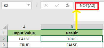
NOT function is an inbuilt function that is categorized under the Logical Function; the logical function operates under a logical test. It is also called Boolean logic or function. Boolean functions are most commonly used along with or in conjunction with other functions, specifically along with conditional test functions (“IF’’ FUNCTION), to create formulas that can evaluate multiple parameters or criteria and produce desired results depending on that criteria. It is used as an individual function or part of the formula and other excel functions in a cell. E.G. with AND, IF & OR function. It returns the opposite value of a given logical value in the formula, NOT function is used to reverse a logical value. If the argument is FALSE, then TRUE is returned and vice versa.

Note: Use NOT function when you want to make sure a value is not equal to one Specific or particular value

It’s a worksheet function; it is also used as part of the formula in a cell along with other excel function

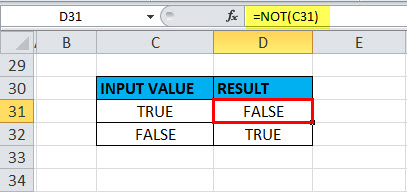
If given with the value TRUE, the Not function returns FALSE
If given with the value FALSE, the Not function returns TRUE

NOT Formula in Excel

Below is the NOT Formula in excel:

=NOT (logical) logical – A value that can be evaluated to TRUE or FALSE

The only parameter in the NOT function is a logical value.

The logical test or argument can be either entered directly, or it can be entered as a reference to a cell that contains a logical value, and it always returns the Boolean value (“TRUE” OR “FALSE”) only.

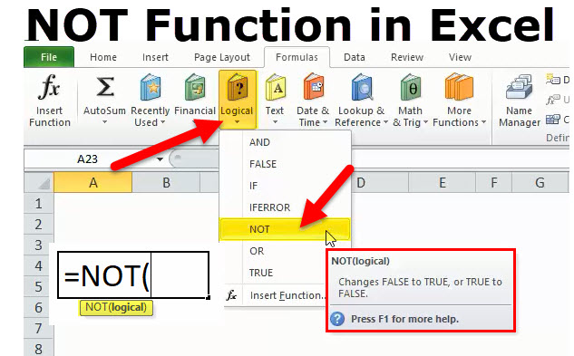
How to Use the NOT Function in Excel?

NOT Function in Excel is very simple and easy to use. Let us now see how to use the NOT function in excel with the help of some examples.

You can download this NOT function Excel Template here – NOT function Excel Template

Example #1 – Excel NOT Function

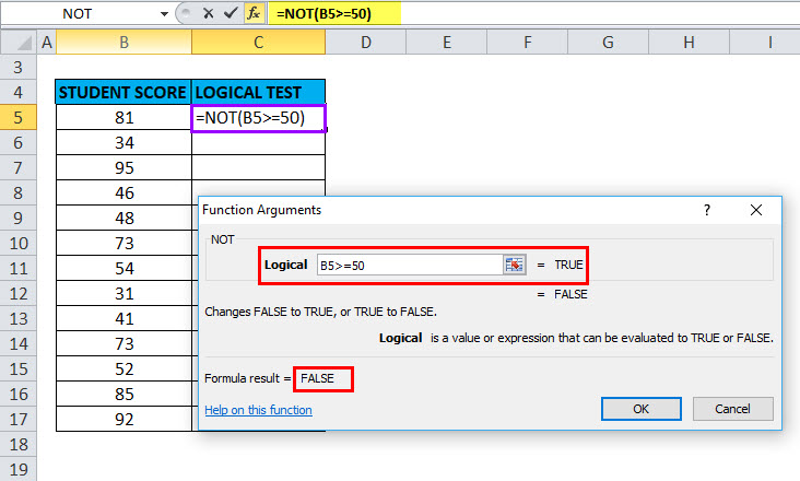
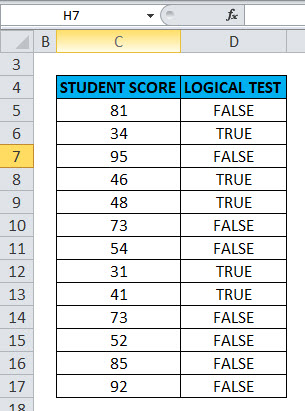
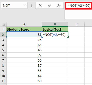
Here a logical test is performed on the given set of values (Student score) by using the NOT function. Here, we will check which value is greater than or equal to 50.

In the table, we have 2 columns, the first column contains student score & the second column is the logical test column, where the NOT function is performed.

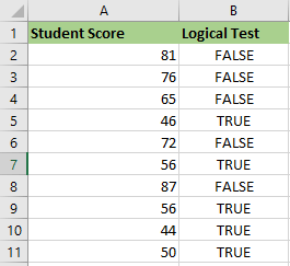
Result: It will return the reverse value if the value is greater than or equal to 50, then it will return FALSE and if the lesser than or equal to 50, it will return TRUE as output.

The result will be as given below:

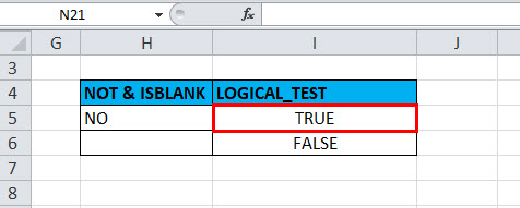
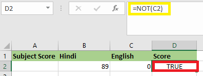
Example #2 – Using NOT Function with ISBLANK

the logical test is performed on the H5 & H6 Cells by using the NOT Function along with ISBLANK function; here will check if cells H5 & H6 is blank OR not using NOT function along with ISBLANK in excel

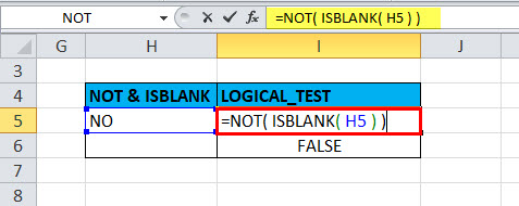
OUTPUT will be TRUE.

Example #3 – NOT Function along with “IF” and “OR” Function

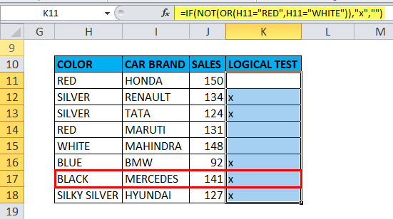
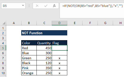
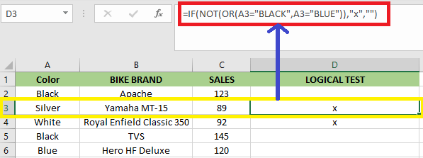
Here the color check is performed for the cars in the below-mentioned table by using NOT Function along with “if” and “or” function

Here we have to sort out color “WHITE” or “RED” from the given set of data

=IF(NOT(OR(H11=”RED”,H11=”WHITE”)),”x”,””) formula is used

This logical condition is applied on a Color column containing any car with color “RED” or “WHITE”,

if the condition is true, then it will return blank as output,

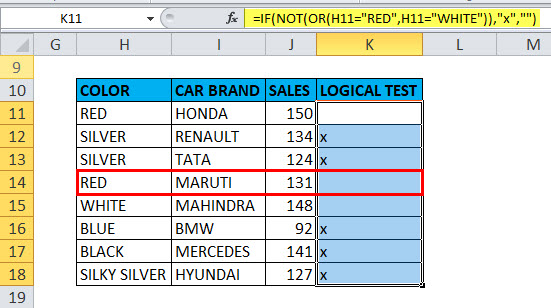
if not true, then it will return x as output

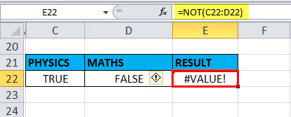
Example #4 – VALUE! Error

It Occurs when the supplied argument is not a logical or numeric value.

Suppose, if we give a range in the logical argument

Selected the range C22:D22 in the logical argument, i.e. =NOT (C22:D22)

a function returns a #VALUE error because the NOT function does not allow any range and can take only a logical test or argument or one condition.

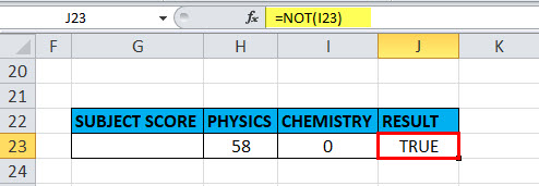
Example #5 – NOT Function for an empty cell or blank or “0”

An empty cell or blank or “0” are treated as false, therefore “NOT” function returns TRUE

Here in the cell “I23”, the stored value is “0” suppose if I apply the “NOT” function with logical argument or value as “0” or “I23”, Output will be TRUE.

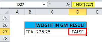
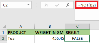
Example #6 – NOT Function for Decimals

When the value is decimal in a cell

Suppose if we take the argument as decimals, i.e. suppose if I apply the “NOT” function with logical argument or value as “225.25” or “c27”, Output will be FALSE.

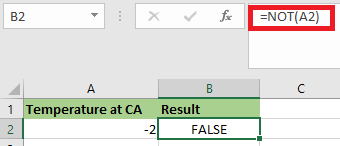
Example #7 – NOT Function for Negative Number

When the value is a negative number in a cell

Suppose if we take the argument as a negative number, i.e. suppose if I apply the “NOT” function with logical argument or value as “-4” or “H27”, Output will be FALSE.

Example #8 – When the value or Reference is Boolean Input in NOT Function

When the value or reference is Boolean input (“TRUE” OR “FALSE”) in a cell.

Here in the cell “C31”, the stored value is “TRUE” suppose if I apply the “NOT” function with logical argument or value as “C31” or “TRUE”, Output will be FALSE. It will be vice versa if the logical argument is “FALSE”, i.e. the NOT function returns the “TRUE” value as output.

Purpose

Reverse arguments or results

Usage notes

The NOT function returns the opposite of a given logical or Boolean value. Use the NOT function to reverse a Boolean value or the result of a logical expression.

When given FALSE, NOT returns TRUE.
When given TRUE, NOT returns FALSE.

Example #1 — not green or red

In the example shown, the formula in C5, copied down, is:

=NOT(OR(B5="green",B5="red"))

The literal translation of this formula is «NOT green or red». At each row, the formula returns TRUE if the color in column B is not green or red, and FALSE if the color is green or red.

Example #2 — Not blank

A common use case for the NOT function is to reverse the behavior of another function. For example, If cell A1 is blank (empty), the ISBLANK function will return TRUE:

=ISBLANK(A1)  // TRUE if A1 is empty

To reverse this behavior, wrap the NOT function around the ISBLANK function:

=NOT(ISBLANK(A1))  // TRUE if A1 is NOT empty

By adding NOT the output from ISBLANK is reversed. This formula will return TRUE when A1 is not empty and FALSE when A1 is empty. You might use this kind of test to only run a calculation if there is a value in A1:

=IF(NOT(ISBLANK(A1)),B1/A1,"")

Translation: if A1 is not blank, divide B1 by A1, otherwise return an empty string («»). This is an example of nesting one function inside another.

Источник

The TRUE function in Excel is intended to indicate a logical true value and returns it as a result of calculations.

The FALSE function in Excel is used to specify a logical false value and returns it accordingly.

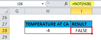
The NOT function in Excel returns the opposite of the specified logical value. For example, writing = NOT (TRUE) will return the result FALSE.

Examples of using the logical functions true, false and not in Excel

Example 1. The Excel spreadsheet stores the phone numbers of various organizations. Calls to some of them are free of charge (code 8800), while the rest are charged at the rate of 1.5 rubles per minute. Determine the cost of calls made.

Data table:

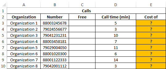
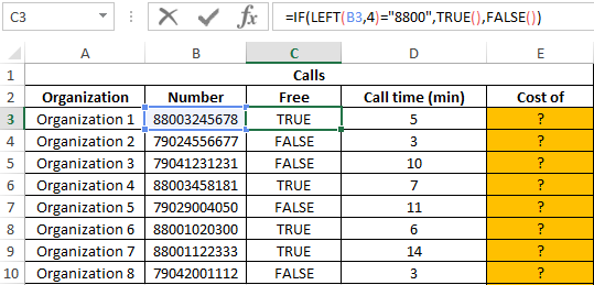
In the “Free” column we display the logical values TRUE or FALSE according to the following condition: is the phone number code equal to “8800”? We introduce the formula in cell C3:

Argument Description:

LEFT (B3; 4) = «8800» — condition for checking the equality of the first four characters of the string to the specified value («8800»).
If the condition is met, the TRUE () function will return a true logical value;
If the condition is not fulfilled, the FALSE () function will return a false logical value.

Similarly, we determine whether the call is free for other rooms. Result:

TRUE.

To calculate the cost, we use the following formula:

Argument Description:

C3 = TRUE () — checking the condition «is the value stored in cell C3 equal to the value returned by the function (logical truth)?».
0- call cost, if the condition is met.
D3 * 1.5 — the cost of the call, if the condition is not met.

Calculation results:

LYING.

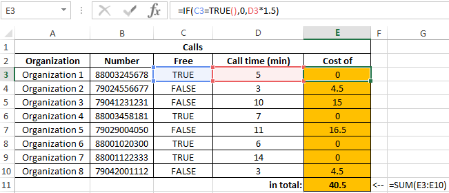
We received the total cost of all calls made by all organizations.

How to calculate the average value of the condition in Excel

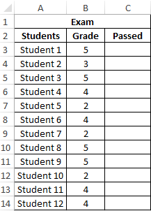
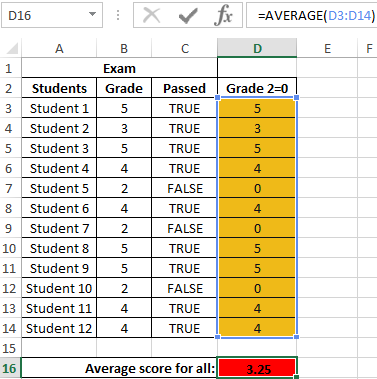
Example 2. Determine the average score for the exam for a group of students, in the composition of which there are students who have failed. It is also necessary to obtain an average assessment of performance only for those students who have passed the exam. The grade of the student who did not pass the exam must be counted as 0 (zero) in the formula for the calculation.

Data table:

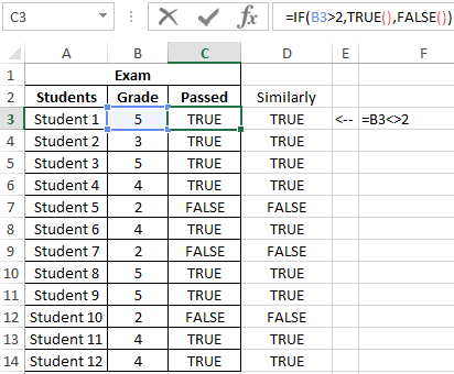
To fill in the “Passed” column, use the formula:

Result of calculations:

IF A.

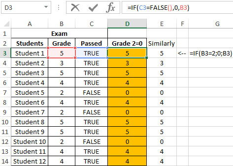
Create a new column in which we rewrite the estimates, provided that grade 2 is interpreted as 0 using the formula:

Result of calculations:

Result.

We determine the average score by the formula:

=AVERAGE(D3:D14)

Result:

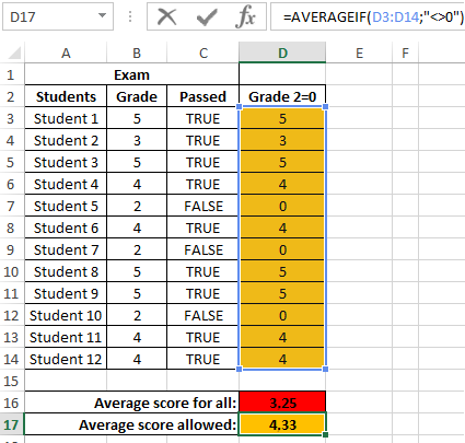
Now we get the average grade point for students who are admitted to the next exams. To do this, we use another logical function AVERAGEIF:

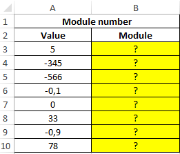
How to get the value module numbers without using the abs function

Example 3. Implement an algorithm for determining the value of the modulus of a number (absolute value), that is, an alternative for the ABS function.

Data table:

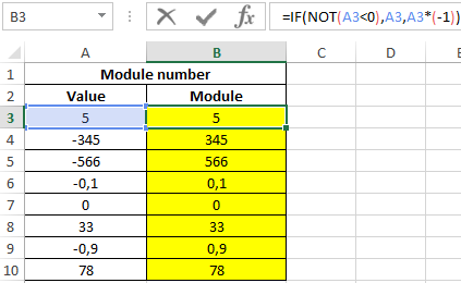
To solve, we use the array formula:

=IF(NOT(A3<0),A3,A3*(-1))

Argument Description:

NOT (A3: A10 <0) — checking the condition “does the number belong to a range of positive values or is it 0 (zero)?”. Without the use of the function, a longer version of the OR record would not be required (A3: A10 = 0, A3: A10> 0);
A3: A10 — the returned number (the corresponding element from the range), if the condition is met;
A3: A10 * (- 1) — the returned number, if the condition is not met (that is, the initial value belongs to the range of negative numbers, to obtain the module, multiply by -1).

Result:

Note: as a rule, the logical values and the functions themselves (TRUE (), FALSE ()) are not explicitly indicated in the expressions, as is done in examples 1 and 2. For example, to avoid intermediate calculations in Example 2, you could use the formula = IF B3 = 2, 0, B3), and also = B3 <> 2.

At the same time, Excel automatically determines the result of calculating the expression B3 <> 2 or B3 = 2, 0, B3 in the arguments of the IF function (logical comparison) and on its basis performs the corresponding action prescribed by the second or third arguments of the IF function.

Features of use of functions true, false, not in Excel

In functions TRUE and FALSE Arguments are absent.

The function does NOT have the following syntax notation:

=NOT( logical value )

Argument Description:

logical is a required argument characterizing one of two possible values: TRUE or FALSE.

Notes:

If the argument logical value of the function is NOT used the number 0 or 1, they are automatically converted to logical values FALSE and TRUE, respectively. For example, the function = NOT (0) returns TRUE, = NOT (1) returns FALSE.
If any numeric value> 0 is used as an argument, the function will NOT return FALSE.
If the only argument of the function is NOT a text string, the function will return the error code #VALUE !.
In computing, a special logical data type is used (in programming, it has the name “Boolean” type or Boolean in honor of the famous mathematician George Boole). This data type operates with only two values: 1 and 0 (TRUE, FALSE).
In Excel, the true logical value also corresponds to the number 1, and the false logical value also corresponds to the numerical value 0 (zero).
The functions TRUE () and FALSE () can be entered in any cell or used in the formula and will be interpreted as logical values, respectively.
Both of the above functions are necessary to ensure compatibility with other software products designed for working with tables.

Download examples of formulas TRUE FALSE and NOT

The function does NOT allow you to expand the capabilities of functions intended to perform a logical test. For example, when using this function as an argument to log_expression of an IF function, you can check several conditions at once.

Источник

Checks if one value is not equal to another

What is the NOT Function?

The NOT Function[1] is an Excel Logical function. The function helps check if one value is not equal to another. If we give TRUE, it will return FALSE and when given FALSE, it will return TRUE. So, basically, it will always return a reverse logical value.

As a financial analyst, the NOT function is useful when we wish to know if a specific condition was not met.

Formula

=NOT(logical)

Where:

Logical (required argument) – The argument should be a logical or numerical value. If the given logical argument is a numeric value, zero is treated as the logical value FALSE and any other numeric value is treated as the logical value TRUE.

How to use the NOT Function in Excel?

NOT is a built-in function that can be used as a worksheet function in Excel. To understand the uses of this function, let us consider a few examples:

Example 1

Suppose we don’t want the red and blue combination for soft toys. We are given the data below:

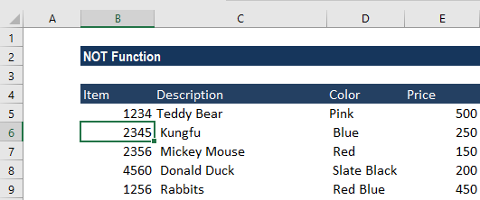
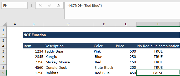
To avoid the Red Blue combination, we will use the formula =NOT(C6=”Red Blue”).

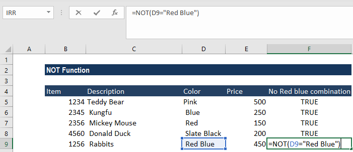
We will get the results below:

If we wish to test several conditions in a single formula, then we can use NOT in conjunction with the AND or OR function. For example, if we wanted to exclude Red Blue and Slate Black, the formula would be =NOT(OR(C2=”Slate black”, C2=”Red Blue”).

Example 2

Suppose we need to put “no bonus” for employees. Basically, we wish to reverse the behavior of some other functions. For instance, we can combine the NOT and ISBLANK functions to create the ISNOTBLANK formula.

The data given to us is shown below:

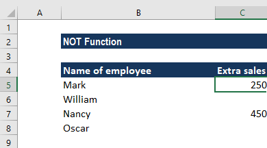
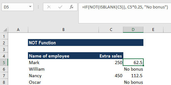
The formula to be used would be =IF(NOT(ISBLANK(C5)), C5*0.25, “No bonus”), as shown below:

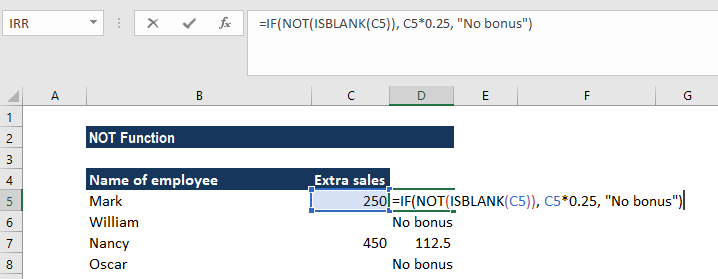
The formula tells Excel to do the following:

If the cell C5 is not empty, multiply the extra sales in C5 by 0.25, which gives the 25% bonus to each salesman who has made any extra sales.
If there are no extra sales – that is, if C5 is blank – then the text, “No bonus”, appears.

We will get the results below:

In essence, this is how we use Logical functions in Excel. We can use this function with AND, XOR, and/or the OR function.

Example 3

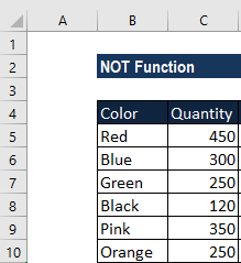
Let’s say we wish to highlight a cell that doesn’t meet specific criteria. In such a scenario, we can use NOT with the IF and OR function. Suppose we received an order to manufacture soft toys of Red and Blue color. The colors are specified by the client and we can’t change them.

We are given the inventory below:

Using the formula =IF(NOT(OR(B5=”red”,B5=”blue”)),”x”,””), we can highlight toys with the two colors:

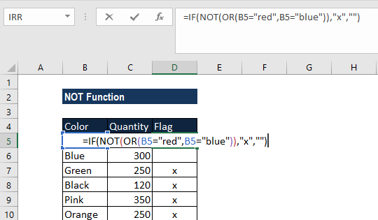
We will get the following result:

Here, we marked inventory that was not of specific colors, that is, which were not Red or Blue.

Using NOT and OR, we will get TRUE if the specified cell is not Red or Blue.

We added an empty string “” so if the result is FALSE, we get X, and nothing if TRUE. We can expand the OR function to add additional conditions if required.

Things to remember

#VALUE! error – Occurs when the given argument is not a logical value or numeric value.

Click here to download the sample Excel file

Additional Resources

Thanks for reading CFI’s guide to important Excel functions! By taking the time to learn and master these functions, you’ll significantly speed up your financial analysis. To learn more, check out these additional CFI resources:

Excel Functions for Finance
Advanced Excel Formulas Course
Advanced Excel Formulas You Must Know
Excel Shortcuts for PC and Mac
See all Excel resources

Article Sources

NOT Function

Источник

NOT Function

Th NOT function in Excel is an inbuilt function. The NOT function belongs to the category of Logical functions. We can use it as a worksheet function; the NOT function can be entered as part of a formula in a worksheet’s cell.

We can use it as an individual function or as a part of a formula and other excel functions in a cell. For example, with IF, AND & OR function. The NOT function is used to reverse a logical value. It returns the opposite value of a given logical value in the formula. If the value of the argument is TRUE, then it will return FALSE and vice versa.

Syntax

The syntax of the NOT function is:

NOT(logical_value)

Arguments or Parameters

logical_value: — An expression that either evaluates TRUE or FALSE. If we used with the expression of TRUE, then FALSE is returned. If used with the expression FALSE, then TRUE is returned.

Returns

If the logical_value is TRUE, then the NOT Function will return
If the logical_value is FALSE, then the NOT function will return

How to Use the NOT Function in Excel?

The NOT function in Excel is quite simple and straightforward to use. Let’s look at some examples of how to use the NOT function in Excel.

Example 1: In this example, the NOT function is used to perform a logical test on the given collection of data (Student score). We’ll check which value is larger than or equal to 60.

The table has two columns: the first column comprises student score & the second column is the logical test column, where the NOT function is performed.

Result: It will give us the opposite result or reverse value. If the value is larger than or equal to 60, the output will be FALSE; if the value is less than or equal to 60. Then the output will be TRUE.

After applying the formula, the result would be:

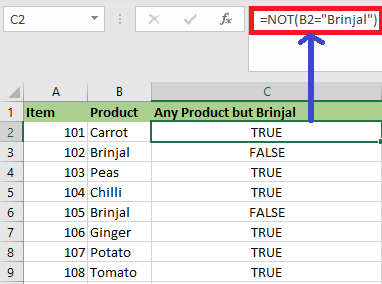
Example 2: Use NOT Function to Exclude Some Specific Values

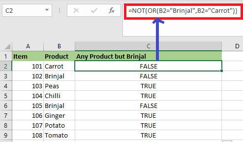
In this example, we have a list of vegetables; we may want to exclude Brinjal, which we don’t like. So, if we use the NOT function, all Brinjal will return FALSE, whereas if we don’t, TRUE will be returned.

The formula we

Note:

1. If we wish to test many conditions in a single formula, we can use NOT with the AND or OR For example, if we need to exclude Brinjal and Carrot, the formula would be:

=NOT(OR(B2=»Brinjal»,B2=»Carrot»))

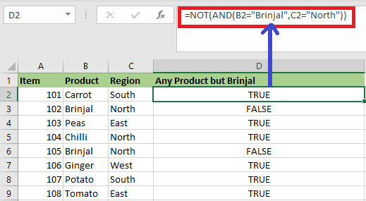
2. Also, if we wish to exclude brinjal from North, use NOT in conjunction with the Excel AND function.

=NOT(AND(B2=»Brinjal»,C2=»North»))

Example 3: Use NOT Function to Deal with Blank Cells

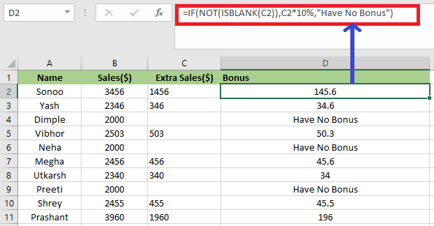
It is another common usage of the NOT function; we can combine the NOT and ISBLANK functions in order to deal with certain blank cells while applying a formula, which is another typical use of the NOT function.

For example, we have a report with employee’s sales, and someone has completed the work excessively. They will receive a bonus if they have extra sales, that equals extra sales*10%. No incentive if their extra sales are blanks.

We may use this formula to combine the NOT and ISBLANK functions, which will give us the following result:

=IF(NOT(ISBLANK(C2*10%,»Have No Bonus»)

Example 4: NOT Function along with «IF» and «OR» Function

In this example, the color check is performed for the bike in the table below using the NOT Function, and the «IF» and «OR» function.

We need to sort out the color «BLUE» or «BLACK» from the given data set.

We will use the below formula:

=IF(NOT(OR(A2=»BLACK»,A2=»BLUE»)),»x»,»»)

This logical condition is applied on a Color column comprising any bike with the color «BLACK» or «BLUE».

If the condition is true, then the output will be blank.

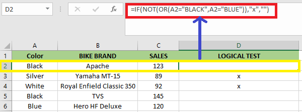
It the condition is not true, then the output will be «x».

Example 5: NOT Function for an Empty Cell or Blank or «0»

The blank cell or empty cell or «0» are considered false, therefore the «NOT» function returns TRUE.

Here in the cell «C2», the stored value is «0» suppose we use NOT function with logical arguments or value as «0» or «C2», the result will be TRUE.

Example 6: NOT Function for Decimals

Suppose the value in the cell is a decimal value. Let’s assume we take the argument as decimals mean if we use the «NOT» function with a logical argument or values as «456.45» or «B2». The result will be FALSE.

Example 7: NOT Function for Negative Number

If the value is a negative number in a cell. Suppose we use a negative number as the parameter; for example, if we use the «NOT» function with a logical argument or value as «-2» or «A2», the result will be FALSE.

Example 8: When the Value or Reference is Boolean Input in NOT Function

If the value or reference is Boolean input («TRUE» OR «FALSE») in a cell. In this example, the cell A2, a FALSE value is stored so, if we use the «NOT» function with logical argument or value as «A2» or «FALSE», the result will be TRUE. If the logical argument is «TRUE,» it will be vice versa means the NOT function returns the «TRUE» value as an output.

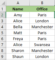
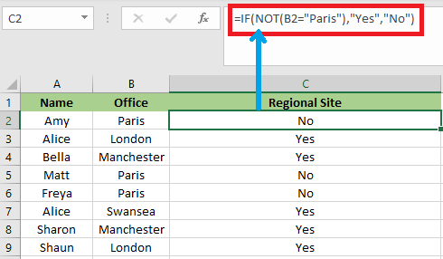
Example 9: Consider the following scenario: We have a head office in Paris and a number of regional offices. If the site is anything other than Paris, then we need to display the word «Yes,» and if it is Paris, we need to display the word «NO.»

The NOT function is nested in the logical test of the IF function given below in order to reverse the TRUE result.

=IF(NOT(B2=»Paris»), «Yes»,»No»)

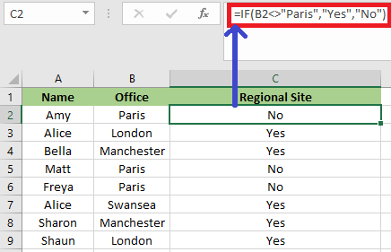
The NOT Logical operator of <> can also be used to do this. Below is an example.

IF(B2<>»Paris»,»Yes»,»NO»)

Example 10: When working with Excel’s information function, the NOT function is helpful. There are a set of Excel functions that check something and return TRUE if the check is successful and FALSE otherwise.

For example, the ISTEXT function will determine whether a cell contains text and return TRUE if it does or FALSE if it does not. The NOT function is useful if it is capable of reversing the result of these functions.

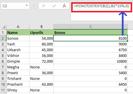
In the below example, we need to pay a salesman 15% of the amount they upsell. However, if they did not upsell anything, the word «None» will appear in the cell, resulting in a formula error.

We used the ISTEXT function to check the Text’s presence. If text is present, then it returns TRUE. Hence the NOT function returns FALSE, And the IF performs its calculation.

=IF(NOT(ISTEXT(B2)),B2*15%,0)

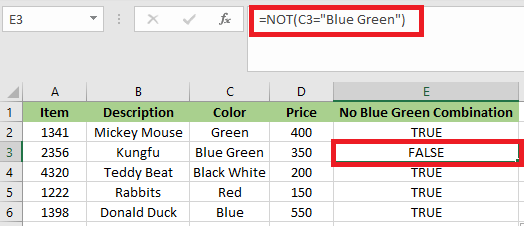
Example 11: Let’s say we do not want our soft toys to be Blue and Green. We have the below dataset:

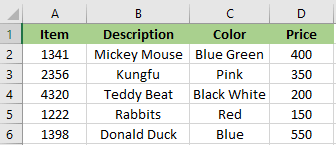
We will use the formula =NOT(C2=»Blue Green») to prevent the Blue Green combo.

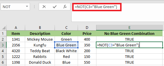
After applying the mentioned formula, we will get the output below:

Источник

Simple IF examples

Common problems

Need more help?

See Also

Need more help?

Want more options?

What is a Logical Function?

IF Function example

Excel Logic functions explained

Practical example

Summary

What is IF Function in Excel?

Table of contents

Syntax of the IF Excel Function

How to Use IF Function in Excel?

Example #1

Example #2

Example #3

Example #4

Example #5

Guidelines for the Multiple IF Statements

Frequently Asked Question

IF Excel Function Video

Recommended Articles

NOT in Excel

NOT Formula in Excel

How to Use the NOT Function in Excel?

Example #1 – Excel NOT Function

Example #2 – Using NOT Function with ISBLANK

Example #3 – NOT Function along with “IF” and “OR” Function

Example #4 – VALUE! Error

Example #5 – NOT Function for an empty cell or blank or “0”

Example #6 – NOT Function for Decimals

Example #7 – NOT Function for Negative Number

Example #8 – When the value or Reference is Boolean Input in NOT Function

Recommended Articles

Purpose

Usage notes

Example #1 — not green or red

Example #2 — Not blank

Examples of using the logical functions true, false and not in Excel

How to calculate the average value of the condition in Excel

How to get the value module numbers without using the abs function

Features of use of functions true, false, not in Excel

What is the NOT Function?

Formula

How to use the NOT Function in Excel?

Example 1

Example 2

Example 3

Things to remember

Additional Resources

Article Sources

NOT Function

Syntax

Arguments or Parameters

Returns

How to Use the NOT Function in Excel?

Example 2: Use NOT Function to Exclude Some Specific Values

Example 3: Use NOT Function to Deal with Blank Cells

Example 4: NOT Function along with «IF» and «OR» Function

Example 5: NOT Function for an Empty Cell or Blank or «0»

Example 6: NOT Function for Decimals

Example 7: NOT Function for Negative Number

Example 8: When the Value or Reference is Boolean Input in NOT Function