
After checking if a cell value exists in a column, I need to get the value of the cell next to the matching cell. For instance, I check if the value in cell A1 exists in column B, and assuming it matches B5, then I want the value in cell C5.
To solve the first half of the problem, I did this…
=IF(ISERROR(MATCH(A1,B:B, 0)), "No Match", "Match")
…and it worked. Then, thanks to an earlier answer on SO, I was also able to obtain the row number of the matching cell:
=IF(ISERROR(MATCH(A1,B:B, 0)), "No Match", "Match on Row " & MATCH(A1,B:B, 0))
So naturally, to get the value of the next cell, I tried…
=IF(ISERROR(MATCH(A1,B:B, 0)), "No Match", C&MATCH(A1,B:B, 0))
…and it doesn’t work.
What am I missing? How do I append the column number to the row number returned to achieve the desired result?
When you need to check if one column value exists in another column in Excel, there are several options. One of the most important features in Microsoft Excel is lookup and reference. The VLOOKUP, HLOOKUP, INDEX and MATCH functions can make life a lot easier in terms of looking for a match.
In this tutorial, we will see the use of VLOOKUP and INDEX/MATCH to check if one values from one column exist in another column.
Check if one column value exists in another column
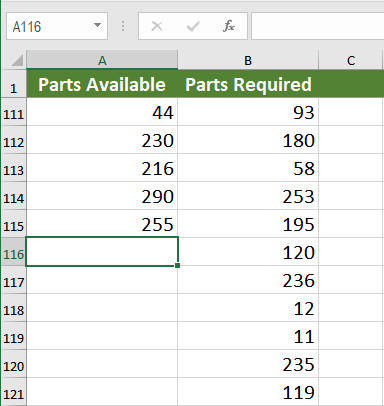
In the following example, you will work with automobile parts inventory data set. Column A has the parts available, and column B has all the parts needed. Column A has 115 entries, and column B has 1001 entries. We will discuss a couple of ways to match the entries in column A with the ones in column B. Column C will output “True” if there is a match, and “False” if there isn’t.
Check if one column value exists in another column using MATCH
You can use the MATCH() function to check if the values in column A also exist in column B. MATCH() returns the position of a cell in a row or column. The syntax for MATCH() is =MATCH(lookup_value, lookup_array, [match_type]). Using MATCH, you can look up a value both horizontally and vertically.
Example using MATCH
To solve the problem in the previous example with MATCH(), you need to follow the following steps:
- Select cell C2 by clicking on it.
- Insert the formula in
"=NOT(ISERROR(MATCH(A2,$B$2:$B$1001,0)))”the formula bar. - Press Enter to assign the formula to C2.

- Drag the formula down to the other cells in column C clicking and dragging the little “+” icon on the bottom-right of C2.
Excel will match the entries in column A with the ones in column B. If there is a match, it will return the row number. The NOT() and ISERROR() functions check for an error which would be and column C will show “True” for a match and “False” if it is not a match.
Check if one column value exists in another column using VLOOKUP
VLOOKUP is one of the lookup, and reference functions in Excel and Google Sheets used to find values in a specified range by “row.” It compares them row-wise until it finds a match. In this tutorial, we will look at how to use VLOOKUP on multiple columns with multiple criteria. The syntax for VLOOKUP is =VLOOKUP(value, table_array, col_index,[range_lookup]).
Example using VLOOKUP
You can check if the values in column A exist in column B using VLOOKUP.
- Select cell C2 by clicking on it.
- Insert the formula in
“=IF(ISERROR(VLOOKUP(A2,$B$2:$B$1001,1,FALSE)),FALSE,TRUE)”the formula bar. - Press Enter to assign the formula to C2.
- Drag the formula down to the other cells in column C clicking and dragging the little “+” icon on the bottom-right of C2.
This will allow Excel to look up all the values in column A and match them with the values of column B. Column C will now show “True” if the corresponding cell in column A has a match in column B, “False” if it does not have a match.
MATCH vs. VLOOKUP – Which is Better?
Between MATCH and VLOOKUP, the better option is MATCH. Not only the formula is simpler, but MATCH is also faster than VLOOKUP when it comes to performance.
MATCH uses a dynamic column reference whereas VLOOKUP uses a static one. If you were to add more columns, with VLOOKUP, you would distort the results. But with MATCH you can easily change the reference when inserting or deleting columns.
Another issue with VLOOKUP is that the lookup value needs to be on the leftmost column of the array, which is not applicable for MATCH. In the previous example, If we had to check if Column C values exist in column A, VLOOKUP would have provided an #N/A error.
Excel has some very effective functions when it comes to checking if values in one column exist in another column. One of these functions is MATCH. It returns the row number based on the lookup value from an array. Another such function is VLOOKUP. It returns the value based on a lookup value from a static array.
When it comes to which function is faster, MATCH is the winner. For its dynamic reference and easy to change array references, MATCH is preferred to check if values in one column also exist in another column.
Most of the time, the problem you need is probably more complex than just simply checking if a value exists in a column. If you want to save hours of researching and frustration, try our Excel Live Chat service! Our Excel experts are available 24/7 to answer any Excel question you have on the spot. The first question is free.
Are you still looking for help with the VLOOKUP function? View our comprehensive round-up of VLOOKUP function tutorials here.
Содержание
- Check If One Column Value Exists in Another Column
- Check if one column value exists in another column
- Check if one column value exists in another column using MATCH
- Example using MATCH
- Check if one column value exists in another column using VLOOKUP
- Example using VLOOKUP
- MATCH vs. VLOOKUP – Which is Better?
- Excel formula that returns row if value is found in a column
- 2 Answers 2
- If found in Column A, display entire row
- 3 Answers 3
- Step 1
- Step 2
- Step 3
- Notes
- Related
- Hot Network Questions
- Subscribe to RSS
- Excel — Need to find if anything from column A is found within column B [duplicate]
- 3 Answers 3
- Excel: If cell contains formula examples
- If cell contains any value, then
- If cell contains text, then
- If cell contains number, then
- If cell contains specific text
- If cell does not contain specific text
- If cell contains text: case-sensitive formula
- If cell contains specific text string (partial match)
- If cell contains certain text, put a value in another cell
- If cell contains specific text, copy it to another column
- If cell contains specific text: case-sensitive formula
- If cell contains one of many text strings (OR logic)
- IF OR ISNUMBER SEARCH formula
- SUMPRODUCT ISNUMBER SEARCH formula
- How this formula works
- If cell contains several strings (AND logic)
- How to return different results based on cell value
- Nested IFs
- Lookup formula
- Vlookup formula
- Practice workbook
- You may also be interested in
Check If One Column Value Exists in Another Column
When you need to check if one column value exists in another column in Excel, there are several options. One of the most important features in Microsoft Excel is lookup and reference. The VLOOKUP, HLOOKUP, INDEX and MATCH functions can make life a lot easier in terms of looking for a match.
In this tutorial, we will see the use of VLOOKUP and INDEX/MATCH to check if one values from one column exist in another column.
Check if one column value exists in another column
In the following example, you will work with automobile parts inventory data set. Column A has the parts available, and column B has all the parts needed. Column A has 115 entries, and column B has 1001 entries. We will discuss a couple of ways to match the entries in column A with the ones in column B. Column C will output “True” if there is a match, and “False” if there isn’t.
Check if one column value exists in another column using MATCH
You can use the MATCH() function to check if the values in column A also exist in column B. MATCH() returns the position of a cell in a row or column. The syntax for MATCH() is =MATCH(lookup_value, lookup_array, [match_type]) . Using MATCH, you can look up a value both horizontally and vertically.
Example using MATCH
To solve the problem in the previous example with MATCH(), you need to follow the following steps:
- Select cell C2 by clicking on it.
- Insert the formula in «=NOT(ISERROR(MATCH(A2,$B$2:$B$1001,0)))” the formula bar.
- Press Enter to assign the formula to C2.
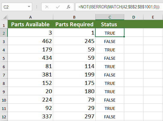
Excel will match the entries in column A with the ones in column B. If there is a match, it will return the row number. The NOT() and ISERROR() functions check for an error which would be and column C will show “True” for a match and “False” if it is not a match.
Check if one column value exists in another column using VLOOKUP
VLOOKUP is one of the lookup, and reference functions in Excel and Google Sheets used to find values in a specified range by “row.” It compares them row-wise until it finds a match. In this tutorial, we will look at how to use VLOOKUP on multiple columns with multiple criteria. The syntax for VLOOKUP is =VLOOKUP(value, table_array, col_index,[range_lookup]) .
Example using VLOOKUP
You can check if the values in column A exist in column B using VLOOKUP.
- Select cell C2 by clicking on it.
- Insert the formula in “=IF(ISERROR(VLOOKUP(A2,$B$2:$B$1001,1,FALSE)),FALSE,TRUE)” the formula bar.
- Press Enter to assign the formula to C2.
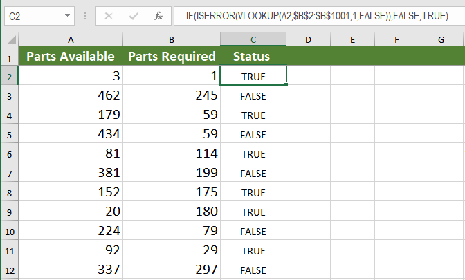
This will allow Excel to look up all the values in column A and match them with the values of column B. Column C will now show “True” if the corresponding cell in column A has a match in column B, “False” if it does not have a match.
MATCH vs. VLOOKUP – Which is Better?
Between MATCH and VLOOKUP, the better option is MATCH. Not only the formula is simpler, but MATCH is also faster than VLOOKUP when it comes to performance.
MATCH uses a dynamic column reference whereas VLOOKUP uses a static one. If you were to add more columns, with VLOOKUP, you would distort the results. But with MATCH you can easily change the reference when inserting or deleting columns.
Another issue with VLOOKUP is that the lookup value needs to be on the leftmost column of the array, which is not applicable for MATCH. In the previous example, If we had to check if Column C values exist in column A, VLOOKUP would have provided an #N/A error.
Excel has some very effective functions when it comes to checking if values in one column exist in another column. One of these functions is MATCH. It returns the row number based on the lookup value from an array. Another such function is VLOOKUP. It returns the value based on a lookup value from a static array.
When it comes to which function is faster, MATCH is the winner. For its dynamic reference and easy to change array references, MATCH is preferred to check if values in one column also exist in another column.
Most of the time, the problem you need is probably more complex than just simply checking if a value exists in a column. If you want to save hours of researching and frustration, try our Excel Live Chat service! Our Excel experts are available 24/7 to answer any Excel question you have on the spot. The first question is free.
Are you still looking for help with the VLOOKUP function? View our comprehensive round-up of VLOOKUP function tutorials here.
Источник
Excel formula that returns row if value is found in a column
I have a list of DNS entries that I need to sort to get the good records.
In sheet1, I have a dump of the raw data, in column 1 is a zone ID which is a number.
In sheet2, I have a column made up of the zone ID’s that I want to keep.
On sheet3 I am looking for a way to take sheet1 column 1, to see if it matches one of the values in sheet2 column 1. If it does, then the result should be the entire row into sheet 3.
Is this possible? Data example is below:
Sheet1 — 4 columns
Sheet2
In column1 is a list of acceptable zone ID’s I want.
Sheet3
If value from sheet1-column1 exists in sheet2-column1, paste the entire row from sheet1.

2 Answers 2
One quick and dirty way to do it is with =COUNTIF(). If the value is found, return the value from cell A1, B1, C1, etc. by filling the formula to the right.
In Sheet 3, Cell A1, enter the following:
Now use the Fill right ( Ctrl + R ) and Fill down ( Ctrl + D ) features to apply the formula to as many cells as required, depending on the number of columns+rows expected in the raw data you have in Sheet 1. If the search is successful, it will fill out the data from that row in Sheet 1.
If the search is unsuccessful, the row will return FALSE. If a cell on sheet 1 does not have data, it will return 0. If desired, you can return blank text («») instead of a FALSE or a 0 with a formula like:
To say it again — this is quick and dirty and will have performance implications if you have a large dataset. You are typically better off putting your raw data in a database — you can then use a Pivot Table or simple SQL queries to extract the data you need in the format required.
Источник
If found in Column A, display entire row
I am trying to do a lookup but VLOOKUP does not seem to be the answer. maybe an INDEX and MATCH formula but I can’t wrap my head around it.
Anyway, I have two tabs, one with data, and the other one will pull parts of the data from the first tab. In tab one my columns look like this (Google Sheets):
In TAB 2, I have the same Columns of Product, Date, Gary, Tom, Mary, but I would like to group their info by product and date. For example, TAB 2 would pull all data that matched Apples and display the entire row. So Tab 2 WOULD give these results:
I would then repeat this for Tab 3 which would pull data for Pears, tab 4 for Oranges, and so on. Of course we will be adding data to this each month so the formula in tab 2 will need to reflect new additions.
3 Answers 3
1) in TAB 2 go to cell A1. right click, and then click data validation.
set up the box as shown below. 
2) in cells B1:E1 put DATE GARY TOM MARY respectively
3)in cell A2 write the following formula: =filter(‘TAB 1′!A:E,’TAB 1’!A:A=A1)
4)choose your fruit from the dropdown box.
5)it might be worht formatting A1 with a yellow fill or something.
This is not going to be possible using standard Excel formulas. To accomplish what you wish I would recommend using several Pivot Tables.
Step 1
Start by selecting the data and navigating to Insert -> Pivot Table in the menu (depending on the version of Excel you are using, the Create PivotTable dialog may differ slightly).

Step 2
Select the PRODUCT column for your filter, the DATE column for your row groups, and the sums of GARY, TOM, and MARY for your values. Set the filter value to Apples (or whichever product you wish to display on this worksheet).

Step 3
Make any desired cosmetic changes to the PivotTable, and then repeat for each worksheet.
Notes
- The PivotTable will not update automatically. If you intend to continue to add rows to your first worksheet, I would recommend setting the Table/Range (in step 1) to something like Sheet1!$A$1:$E$1000 . Then, when an edit is made you can click the Refresh button in the menu to refresh the data.

- If you don’t want to have to refresh all tables manually, you can build a macro that will do so automatically.
I suggest using PivotTables, as opposed to formulas. You can name the data range you use which can be large enough to accommodate future entries and create a PivotTable on each tab quite easily — select the data or named range and do Insert -> PivotTable. Then, within the PivotTable Field List, use the «Choose fields to add to report:» filters and select the specific product you want for a given tab. This would work best if there are only a few handfuls of items as managing 100’s of different products or product types may become tedious.
By using a large enough range, you can add data to the set and/or range and use the «Refresh All» button under the ‘Data’ tab to update the workbook.
Chandoo.org provides some great resources for PivotTable use. Also, when I first started I was fond of fiveminutelessons.com. To be honest, a quick Google search should turn up some decent help topics
Hot Network Questions
To subscribe to this RSS feed, copy and paste this URL into your RSS reader.
Site design / logo © 2023 Stack Exchange Inc; user contributions licensed under CC BY-SA . rev 2023.3.17.43323
By clicking “Accept all cookies”, you agree Stack Exchange can store cookies on your device and disclose information in accordance with our Cookie Policy.
Источник
Excel — Need to find if anything from column A is found within column B [duplicate]
Basicaly, I have 2 lists of email addresses in Excell.
I need a way to find out which email addresses in Column A aren’t found in Column B, and preferably output the results in, either a new sheet, or in Column C.
Than after that I need to be able to find which email addresses in Column B aren’t found in Column A (if any) and output that list into, either a new sheet or Column D.
How can I do this?
3 Answers 3
In either a new sheet or column C use a combination of VLOOKUP() and IFERROR() and drag that formula for every line of A.
=IF(ISERROR(VLOOKUP(A1, $B$1:$B$1995, 1, 0)), A1 & » NOT FOUND IN COLUMN B», «FOUND IN B»)
This will return two different messages depending on if the e-mail was found or not in B.

Why not copy paste the data from column B onto the end of column A? Then set the conditional formatting for the column to highlight all items whose count exceeds one. Use this formula, » =countif($A$1:A1,A1)>1 «, without the quotes. Make sure the whole column is selected when doing this.
Another method for maintaining the separation of data. In column C use a formula like this =IF(ISERROR(VLOOKUP(A1,$B$1:$B$100,1,0)),A1,»») ; change the ranges to match your data ranges. Then fill down the formula until the end of data in column A. To fill down, select the desired range and press ‘Cntl+D’. Repeat this for column D but swap the A and B references in the formula and fill down until the bottom of the column B data. This will result in data in columns C & D that list the unique values. Copy and paste these values, be sure to paste as values if the default paste is used Excel will paste the formulas and not the data, into another set of columns (E & F) or the same columns, then sort each column to eliminate the spaces.
Источник
Excel: If cell contains formula examples
 by Svetlana Cheusheva, updated on March 17, 2023
The tutorial provides a number of «Excel if contains» formula examples that show how to return something in another column if a target cell contains a required value, how to search with partial match and test multiple criteria with OR as well as AND logic.
One of the most common tasks in Excel is checking whether a cell contains a value of interest. What kind of value can that be? Just any text or number, specific text, or any value at all (not empty cell).
There exist several variations of «If cell contains» formula in Excel, depending on exactly what values you want to find. Generally, you will use the IF function to do a logical test, and return one value when the condition is met (cell contains) and/or another value when the condition is not met (cell does not contain). The below examples cover the most frequent scenarios.
If cell contains any value, then
For starters, let’s see how to find cells that contain anything at all: any text, number, or date. For this, we are going to use a simple IF formula that checks for non-blank cells.
For example, to return «Not blank» in column B if column A’s cell in the same row contains any value, you enter the following formula in B2, and then double click the small green square in the lower-right corner to copy the formula down the column:
The result will look similar to this: 
If cell contains text, then
If you want to find only cells with text values ignoring numbers and dates, then use IF in combination with the ISTEXT function. Here’s the generic formula to return some value in another cell if a target cell contains any text:
Supposing, you want to insert the word «yes» in column B if a cell in column A contains text. To have it done, put the following formula in B2:
=IF(ISTEXT(A2), «Yes», «») 
If cell contains number, then
In a similar fashion, you can identify cells with numeric values (numbers and dates). For this, use the IF function together with ISNUMBER:
The following formula returns «yes» in column B if a corresponding cell in column A contains any number:
=IF(ISNUMBER(A2), «Yes», «») 
If cell contains specific text
Finding cells containing certain text (or numbers or dates) is easy. You write a regular IF formula that checks whether a target cell contains the desired text, and type the text to return in the value_if_true argument.
For example, to find out if cell A2 contains «apples», use this formula:
=IF(A2=»apples», «Yes», «») 
If cell does not contain specific text
If you are looking for the opposite result, i.e. return some value to another column if a target cell does not contain the specified text («apples»), then do one of the following.
Supply an empty string («») in the value_if_true argument, and text to return in the value_if_false argument:
=IF(A2=»apples», «», «Not apples»)
Or, put the «not equal to» operator in logical_test and text to return in value_if_true:
=IF(A2<>«apples», «Not apples», «»)
Either way, the formula will produce this result: 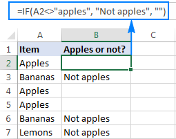
If cell contains text: case-sensitive formula
To force your formula to distinguish between uppercase and lowercase characters, use the EXACT function that checks whether two text strings are exactly equal, including the letter case:
=IF(EXACT(A2,»APPLES»), «Yes», «») 
You can also input the model text string in some cell (say in C1), fix the cell reference with the $ sign ($C$1), and compare the target cell with that cell:
=IF(EXACT(A2,$C$1), «Yes», «») 
If cell contains specific text string (partial match)
We have finished with trivial tasks and move on to more challenging and interesting ones 🙂 In this example, it takes three different functions to find out whether a given character or substring is part of the cell contents:
Working from the inside out, here is what the formula does:
- The SEARCH function searches for a text string, and if the string is found, returns the position of the first character, the #VALUE! error otherwise.
- The ISNUMBER function checks whether SEARCH succeeded or failed. If SEARCH has returned any number, ISNUMBER returns TRUE. If SEARCH results in an error, ISNUMBER returns FALSE.
- Finally, the IF function returns the specified value for cells that have TRUE in the logical test, an empty string («») otherwise.
And now, let’s see how this generic formula works in real-life worksheets.
If cell contains certain text, put a value in another cell
Supposing you have a list of orders in column A and you want to find orders with a specific identifier, say «A-«. The task can be accomplished with this formula:
Instead of hardcoding the string in the formula, you can input it in a separate cell (E1), the reference that cell in your formula:
For the formula to work correctly, be sure to lock the address of the cell containing the string with the $ sign (absolute cell reference). 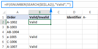
If cell contains specific text, copy it to another column
If you wish to copy the contents of the valid cells somewhere else, simply supply the address of the evaluated cell (A2) in the value_if_true argument:
The screenshot below shows the results: 
If cell contains specific text: case-sensitive formula
In both of the above examples, the formulas are case-insensitive. In situations when you work with case-sensitive data, use the FIND function instead of SEARCH to distinguish the character case.
For example, the following formula will identify only orders with the uppercase «A-» ignoring lowercase «a-«.
=IF(ISNUMBER(FIND(«A-«,A2)),»Valid»,»») 
If cell contains one of many text strings (OR logic)
To identify cells containing at least one of many things you are searching for, use one of the following formulas.
IF OR ISNUMBER SEARCH formula
The most obvious approach would be to check for each substring individually and have the OR function return TRUE in the logical test of the IF formula if at least one substring is found:
Supposing you have a list of SKUs in column A and you want to find those that include either «dress» or «skirt». You can have it done by using this formula:
=IF(OR(ISNUMBER(SEARCH(«dress»,A2)),ISNUMBER(SEARCH(«skirt»,A2))),»Valid «,»») 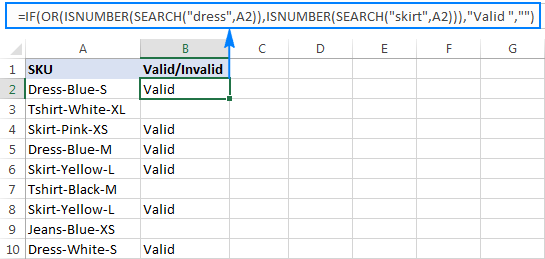
The formula works pretty well for a couple of items, but it’s certainly not the way to go if you want to check for many things. In this case, a better approach would be using the SUMPRODUCT function as shown in the next example.
SUMPRODUCT ISNUMBER SEARCH formula
If you are dealing with multiple text strings, searching for each string individually would make your formula too long and difficult to read. A more elegant solution would be embedding the ISNUMBER SEARCH combination into the SUMPRODUCT function, and see if the result is greater than zero:
For example, to find out if A2 contains any of the words input in cells D2:D4, use this formula:
Alternatively, you can create a named range containing the strings to search for, or supply the words directly in the formula:
Either way, the result will be similar to this: 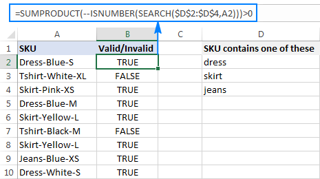
To make the output more user-friendly, you can nest the above formula into the IF function and return your own text instead of the TRUE/FALSE values:
=IF(SUMPRODUCT(—ISNUMBER(SEARCH($D$2:$D$4,A2)))>0, «Valid», «») 
How this formula works
At the core, you use ISNUMBER together with SEARCH as explained in the previous example. In this case, the search results are represented in the form of an array like . If a cell contains at least one of the specified substrings, there will be TRUE in the array. The double unary operator (—) coerces the TRUE / FALSE values to 1 and 0, respectively, and delivers an array like <1;0;0>. Finally, the SUMPRODUCT function adds up the numbers, and we pick out cells where the result is greater than zero.
If cell contains several strings (AND logic)
In situations when you want to find cells containing all of the specified text strings, use the already familiar ISNUMBER SEARCH combination together with IF AND:
For example, you can find SKUs containing both «dress» and «blue» with this formula:
Or, you can type the strings in separate cells and reference those cells in your formula:
=IF(AND(ISNUMBER(SEARCH($D$2,A2)),ISNUMBER(SEARCH($E$2,A2))),»Valid «,»») 
As an alternative solution, you can count the occurrences of each string and check if each count is greater than zero:
The result will be exactly like shown in the screenshot above.
How to return different results based on cell value
In case you want to compare each cell in the target column against another list of items and return a different value for each match, use one of the following approaches.
Nested IFs
The logic of the nested IF formula is as simple as this: you use a separate IF function to test each condition, and return different values depending on the results of those tests.
Supposing you have a list of items in column A and you want to have their abbreviations in column B. To have it done, use the following formula:
=IF(A2=»apple», «Ap», IF(A2=»avocado», «Av», IF(A2=»banana», «B», IF(A2=»lemon», «L», «»)))) 
For full details about nested IF’s syntax and logic, please see Excel nested IF — multiple conditions in a single formula.
Lookup formula
If you are looking for a more compact and better understandable formula, use the LOOKUP function with lookup and return values supplied as vertical array constants:
For accurate results, be sure to list the lookup values in alphabetical order, from A to Z.
=LOOKUP(A2,<«apple»;»avocado»;»banana»;»lemon»>,<«Ap»;»Av»;»B»;»L»>) 
Compared to nested IFs, the Lookup formula has one more advantage — it understands the wildcard characters and therefore can identify partial matches.
For example, if column A contains a few sorts of bananas, you can look up «*banana*» and have the same abbreviation («B») returned for all such cells:
=LOOKUP(A2,<«apple»;»avocado»;»*banana*»;»lemon»>,<«Ap»;»Av»;»B»;»L»>) 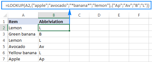
Vlookup formula
When working with a variable data set, it may be more convenient to input a list of matches in separate cells and retrieve them by using a Vlookup formula, e.g.:
=VLOOKUP(A2, $D$2:$E$5, 2,FALSE ) 
This is how you check if a cell contains any value or specific text in Excel. Next week, we are going to continue looking at Excel’s If cell contains formulas and learn how to count or sum relevant cells, copy or remove entire rows containing those cells, and more. Please stay tuned!
Practice workbook
You may also be interested in
Table of contents
Hi,
I need to find the text in list of data which contain specific text to return a specific value and am trying to use IF function with combinations of AND and ISNUMBER, SEARCH but it does not return expected result. can you teach me how can I solve this pls?
Hi!
Your information is not enough to help. I don’t have your data and I don’t know what kind of result you want to have.
What to do if the «IF» command overwrites cells?
For example, for participant ID N840, age 24 is needed. I am using =IF(A2=»N840″, «24», «»), and it works well.
However, for a different participant, ID N860, the age needs to be 26. When writing the command, it overwrites the previous one, leaving it blank.
Important to mention that I have multiple data from each participant (longitudinal data).
Thank you very much.
Hi!
I don’t really understand what your problem is. Perhaps this article will be helpful to you: How to copy formula in Excel with or without changing references. If this does not help, explain the problem in detail.
Thank you for your prompt response. I will try and explain it thoroughly:
I have 20 participants (each has an ID code, e,g., N840), that filled out the same questionnaire over time (meaning, for each participant, I have roughly 16 responses, that is 16 excel rows). The particiapnts filled in their demographic data in a different questionnaire.
I want to assign each participant his age across all of his responses. I am doing the following:
For example, the data for participant N840 is located in excel rows 2, 4, 9, and so on. I am using the following command to enter his age across all rows: IF(B2=»N840″, «24», «»). It works and fills the column where needed (e.g., rows 2, 9) at the age of 24.
However, when I create a formula for the next participant (A840) in the adjacent row, i.e., IF(B3=»A840″, «25», «»), it deletes the age data for the previous participants.
I hope it is more clear now.
What can/should I do differently?
Create a table with 2 columns: ID code and age. You can get the age of each participant from this table using the VLOOKUP function. For example,
A1 — participant ID code
For more instructions and examples, see this article: Excel VLOOKUP function tutorial with formula examples.
I hope it’ll be helpful. If something is still unclear, please feel free to ask.
I’m trying to find the best formula for my scenario,
I need to search cell B2 — if it contains one word and contains one cell, then result another cell.
Currently, the below formula works
=IF(AND(ISNUMBER(SEARCH(«H-Type»,B2)),ISNUMBER(SEARCH($AW$2,B2))),$AZ$2,»»)
I need to add, if this is false, then continue searching for results with alternative options
Like (SEARCH(«P Type»,B2)),ISNUMBER(SEARCH($AW$3,B80))),$AZ$3,»») and continue until result is found
Sample/search options for B2:B1840 fields — maybe 30 different text options like «H-Type» or «P-Type»
H-TypeВ® (18″/450mm) X with X and X
P-Type (90″/2200mm) X with X and X
Sample options for AW2:AW24 cells
12″
18″
90″ etc
Results — Table(called Sizes) between AZ2:BD24 depending on result of text option
Example. If «H-Type» then result within AZ:2AZ24, if «P-Type» then result within BB2:BB24 etc
Actual value of result will be single numbers between 2 — 20
So, I need to check cell B2 contains «H-Type» and AW2, if yes show value in AZ2, if no check if B2 contains «H-Type» and AW3, if yes show value AZ3, if no continue until a match is found. There should always be a match to one of the combinations between each text and cell option.
or
If B2 contains «H-Type» and AW2 then VLOOKUP(B2,Sizes,4,FALSE))
If B2 contains «P-Type» and AW2 then VLOOKUP(B2,Sizes,6,FALSE))
I hope that all makes sense,
I think this will be way to many conditions for one formula, is this formula even possible?
Hello!
I recommend using the IFS function instead of the IF function for many alternative searches. For more information, read this article: The new Excel IFS function instead of multiple IF.
For example, try this formula:
=IFS(AND(ISNUMBER(SEARCH(«H-Type»,B2)),ISNUMBER(SEARCH($AW$2,B2))),$AZ$2, AND(ISNUMBER(SEARCH(«P Type»,B2)),ISNUMBER(SEARCH($AW$3,B80))),$AZ$3)
I hope my advice will help you solve your task.
I am working on a running document. I am attempting to create a formula that will subtract from two cells IF text or a number is present in a different cell. For example if text or a number is present in V3 or U3, then perform E3-D3. My formula looks like:
But it does not work.
Hello!
The ISTEXT function only checks the text in the cell, not the number. Try ISBLANK function.
Hello, I need a help in «improv»ing a formula.
I have something like this in an if: IF(OR(C13=»Closed»,C13=»Dropped»,C13=»Suspended»), ##DoThis##, ##DoThat## )
Can I rewrite it in a manner where I need to type C13 only once? like..
IF(SOMEFUNCTION(C13,»Closed»,»Dropped»,»Suspended»), ##DoThis##, ##DoThat## )
Reason being, there may be another string that might have to be checked for C13, and I am too lazy to type in C13 again ! 🙂
I am aware that I can probably write it like:
IF(ISNUMBER(FIND(C13,»Closed»&Dropped»&»Suspended»)), ##DoThis##, ##DoThat## )
But, is this the only option?
Thank you very much.
Hello!
Instead of a formula
OR(C13=»Closed»,C13=»Dropped»,C13=»Suspended»)
use
OR(C13=<«Closed»,»Dropped»,»Suspended»>)
I am trying to add this function; where a particular range of numbers results in a specific text response
for example:
scores in one column within the following ranges (98) will result the following descriptors in the adjacent column (exceptionally low, below average, low average, average, high average, above average, exceptionally high).
how do i write out a command?
Hi!
You can learn more about multiple IF conditions in Excel in this article on our blog: Nested IF in Excel – formula with multiple conditions.
Excellent!
Thank you!!
Please help provide the formula if a range of cells contain the letters BR, then I would like the sum of another range of cells of just containing BR to return the value, thank you.
Hello!
To find the sum of the cells by condition, try using the SUMIF function. I hope it’ll be helpful. If this is not what you wanted, please describe the problem in more detail.
Exactly what I needed thank you!
I’m currently using the below formula to extract/filter out data from a master sheet to another sheet, however this gives blank cells/rows in between which I don’t want. I tried adding VLOOKUP to the formula but unsuccessful (still noob at using LOOKUP).
May I seek your help on how to edit the formula, so that I can have a list of results without blank cells/rows in between please?
Thanks in advance!
Hello!
To get a list of values by condition, I recommend using the FILTER function
For example,
You can find the examples and detailed instructions here: Excel FILTER function — dynamic filtering with formulas
I have a text string including multiple words and I would like the return value to be different for each IF. For example Statement=send letter with word USD and CAD.If the string includes USD then abbreviate US and if CAD is found then abbreviate CA.
Hi!
To understand what you want to do, give an example of the source data and the desired result.
=IF(ISLBANK(P5),(ISNUMBER(P5), «Done», «Pending»))
I have alredy applied this formula in A5 Cell. So my A5 row is now fill with this formula value. But when my B5 cell value is blank, Then I need to blank also my A5 Cell. How can I applied that with this formula?
HI! I am wondering if you guys can help.. Doing some report for my team
Conditions if scores are from 6.42-7.41 = 5 Coins. if 7.42 — 8;49, 10 coins and if 8.50 — 300, 15 coins.. I used
B22 = 5
B23 = 10
B24 = 15
C3 is 25.53 but result still is 5. Should be 15. Not sure if there’s a mistake with my formula. Thank you.
Hi!
You can find the examples and detailed instructions here: Nested IF in Excel – formula with multiple conditions. Try this formula:
If cell G4 contains wording Baseline
Cell H19 mustn’t add 5% (Costing)
If cell G4 contains wording Project
Cell H19 must add 5% (Costing)
Hi!
You can find the answer to your question in this article: Nested IF in Excel – formula with multiple conditions.
Need formula in Col B. eg. if B2 contains state listed in D2:D8 & Name of that state should be automatically added there.
| | | |
| A | B | C |
——————————————————————————————————————————————
| | | |
| | | |
| Address | States | Total States |
| | | |
| | | |
| Los Angeles, California, United States, 91311 | California | California |
| | | |
| Santa Clarita, California, United States, 91355-5078 | California | Florida |
| | | |
| Saint Petersburg, Florida, United States, 33701 | Florida | Texas |
| | | |
| Walnut Creek, California, United States, 94596-4410 | California | XYZ |
| | | |
| Roseville, California, United States, 95661 | California | XYZ1 |
| | | |
| Lake Forest, California, United States, 92630-8870 | California | XYZ2 |
| | | |
| Houston, Texas, United States, 92660 | Texas | XYZ3 |
Hi!
Sorry, I do not fully understand the task.
Please clarify your specific problem or provide additional details to highlight exactly what you need. What result do you want to get?
Please advise a number check formula that will yield «if lesser then» in a string scenario (dimensions in a cell) to find out if any of the numbers in their position are lesser then 5.
Cell Example: 11 x 3 x 4
Cell Formula Result: false true true
Hello!
To extract all numbers from text, use a user-defined function RegExpExtract. You can find the examples and detailed instructions here: How to extract substrings in Excel using regular expressions (Regex).
I have an excel file where a cell can contain 2 languages (Arabic and English). Is there a way to highlight which of these cells in the sheet have 2 languages. Also, is there a way to further determine if the English language (word) starts at the beginning of the sentence.
The problem is that we are working on a project to create an app, some sentences should include popular english words followed by arabic words. But whenever the sentence start with english, a problem appears in our user interface. That’s why I need to determine which sentences in the cell start with and English word.
Hello!
You can determine the ANSI code of the first character in a text. The ASCII value of the lowercase alphabet is from 97 to 122. And, the ASCII value of the uppercase alphabet is from 65 to 90. To do this, use the CODE function.
See CODE function example here.
I hope my advice will help you solve your task.
Thank you so much Alexander. This helped me a lot!
Hi, need help with a formula, please:
If cell contains certain text, put a value in another cell: So that would be =IF(ISNUMBER(SEARCH(«Sub»,A2)),»Approve»,»»)
But, I would like to use such a formula to look for «Sub» in a range of cells, for example, A2:F2 (1st case scenario), and then in a different instance, to look for «Sub» in a group of cells — A2, C2, D2 and G2 (2nd case scenario).
Thank you very much in advance.
Hello!
Try using the SUM formula to get the search result in a range.
I hope it’ll be helpful.
Kind greetings and thank you very much for your kind help / response. I tried the equation that you helped provide above but it still provides a blank response, even when one of the cells contains «Sub».
In this case, I’m trying to approve the the row #3 because one of the cells from C3 to G3, in this case E3, contains the string «Sub».
A B C D E F G H
1 Alt ID Plans CovA CovB CovC CovD CovE Approval
2 101020 Pol3 Plan11 Coord2e
3 907030 Pol Sub5a Alt24
4 805050
5 778050 Plan88 Sub7d Coord2
6 232520 Sub4 ALt4 Plan6
7 357031 Plan2d Sub7e
So, I used =IF(SUM(—ISNUMBER(SEARCH(«Sub»,C3:G3))),»Approve»,»») but it still gives a blank response.
Thank you again, in advance.
Hi!
I have used your data. The formula works.
Hi, thank you very much for your kind help. I read one of your blogs on Excel ISNUMBER function with formula examples, under conditioning with SUMPRODUCT and it helped.
The equation I’m using now is =IF(SUMPRODUCT(—ISNUMBER(SEARCH(«Sub»,C3:G3))),»Approve»,»») and it is helping with what I needed to do.
Again, your very kind help is much appreciated.
Hello!
You didn’t specify this, but I’m assuming you’re working with Excel 2019 or 2016. The formula returns an array that needs to be summed. In Excel 365, you do not need to do this.
Sorry about that; and yes, I’m working with Excel 2019.
Again, I thank you.
I am new to extended formulas. I usually manage with Vlook Up and Pivots. I am trying to show value of cell B2 in cell C2, if Text in Cell A2 is specific and if not, then value in Cell C2 must reflect «0» / zero. Likewise, for Row no.s 3, 4, 5, .
Eg., A2 value is «Opening Balance», B2 value is «100» then C2 must reflect the value of Cell B2 i.e., «100». But if A2 value is NOT «Opening Balance» then C2 must reflect «0» / zero in numerical value. Please help me.
A B C D E F
Transactions Amount Opening Balance Invoice Debit Note Receipt
1 Opening Balance 100.00 100.00 0 0 0
2 Invoice 248.00 0 248.00 0 0
3 Debit Note 10.00 0 0 10.00 0
4 Receipt 238.00 0 0 0 238.00
Hello!
For your task, you can use the IF function.
IF(A2=»Opening Balance», B2, 0)
If the suggested formula doesn’t work for your case, feel free to describe it in detail.
Great information. Is it possible to put a formula in a cell that tests a different cell and places text in a 3rd cell ?
Example: Formula is in cell E1, testing cell A1 is equal to «Test», setting cell B1 equal to «Yes»
Cell B1 has other text in it until cell A1 has been changed to «Test» manually.
If, Then , Else structure but being able to specify the cells for the then and Else output.
I used this structure but can not specify a target cell
Cell B1 is =IF(ISNUMBER(SEARCH(«Test,A1)),»Yes»,»No») will set B1 to Yes or No
but wish to add target cells for results:
Formula is in cell E1 =IF(ISNUMBER(SEARCH(«Test,A1)),(«Yes»,B1),(«No»,C1)) Target cells are B1 and C1
I know how to do it in Macro but then need to run the macro. I wanted it to happen without running or adding macro.
Thanks,
Vin
Hi!
It has already been written many times in this blog that an Excel formula can only change the value of the cell in which it is written. For all other tasks, use VBA.
Hello, I would like to seek help. If a cell has a text value: then perform another formula else blank
Hi!
To check if a value is text, use the Excel IF ISTEXT formula.
I know how to count a series of keywords in Excel. I use this formula: =SUMPRODUCT(—ISNUMBER(SEARCH($CE$2:$CE$43,(G2:AP2))))
However, what would be the Excel formula if I want to count the number of keywords that exist only within +/-3 words around «risk» in the selected rows?
Consider this sentence: «Political uncertainty generates economic risk which stagnates economic activities.» If my keywords are «political», «uncertainty», «stagnates», and economic», the total number of keywords within +/- 3 words around «risk» will be 3, i.e., «uncertainty», «stagnates», and «economic». «political» will be excluded since it is out of range.
IF the cell contains numbers and characters and without numbers , how can i filter only character cells please help me
Hello!
I recommend using a custom function REGEXMATCH. You can find the examples and detailed instructions here: How to use regex to match strings in Excel. You can filter on the TRUE value that this function will return.
this function selected another word that we don’t need because the two (alphabet) first of this word are the same (ALbendazole and ALcid) any suggestions pls?
Hi!
I can’t guess which formula and which values you are using. Please describe it in detail and I will try to help.
Please help to write a formula for the below
If I update the formula in I2 cell to =IF(SEARCH(«HOSB»,H2),»PO»,»»), the result is coming correctly, but if I change it to =IF(SEARCH(«HOSB»,H2),»PO»,IF(SEARCH(«HONB»,H2),»Non PO»,IF(SEARCH(«HOCB»,H2),»Contract», IF(SEARCH(«HORB»,H2),»Retention»,»»)))) I am getting an error stating #VALUE!
Hello!
If the text is not found in the cell, the SEARCH function will return an error. Add an ISNUMBER function to your formula. In case of a successful search, it will return TRUE, in case the text is not found, it will return FALSE.
=IF(ISNUMBER(SEARCH(«HOSB»,H2)),»PO», IF(ISNUMBER(SEARCH(«HONB»,H2)),»Non PO», IF(ISNUMBER(SEARCH(«HOCB»,H2)),»Contract», IF(ISNUMBER(SEARCH(«HORB»,H2)),»Retention»,»»))))
I intend to use this formula and I got a comment «This formulate use more level of nesting than you can use in the current file formate.» How to fix this formula?
Hello!
The nested IF function has a limit. In Excel 2003 this is 7 levels, in later versions, it is 64 levels. Read more in the article: Excel nested IF statement — multiple conditions in a single formula.
Kindly help please
A have a row for the report headers and below it a a row that says it is Mandatory or optional.
How so i check if the mandatory columns have value?
Hello!
To determine the cells that have values, you can use a combination of functions NOT(ISBLANK(A1)).
Please have a look at this article — Excel formula: if cell is not blank then.
I hope it’ll be helpful.
Hi! Thanks for the response.
But how do i make it dependent on the mandatory/optional row?
For example if the following column headers are the following: name, address,mobile,birthday.( last column is the checking, row complete?)
And then on the row below , all the fields are mandatory except for the birthday.
* row complete value should be TRUE if the mandatory cells are populated.
Hi!
Combine all of these conditions in an IF function as described in this guide: Excel IF statement with multiple AND/OR conditions.
IF(AND(NOT(ISBLANK(A1)),NOT(ISBLANK(B1)),NOT(ISBLANK(C1))),TRUE,FALSE)
It would somehow look like this.
But i dont get how will the code be dependent on the second row. (By checking “Mandatory “)
Name Address Birthday Mobile Row complete?
Mandatory Mandatory Optional Mandatory
James ABC street 8171777 True
Alice Aaa streeat 10/10/1970 81666 True
Hi!
If I understand the problem correctly, you need to copy the formula to the second line and beyond.
Hi, the problem is that i need to check for row 2 as well( mandatory optional)
Starting from row 3( i need to check if there are blank values from the cells tagged as mandatory)
I actually have around 20 headers ( lets say from a1 to t1) and from a2 to t2 it says mandatory or optional.
Hi!
Use in the formula the addresses of only those cells that are mandated.
Hello,
I am trying to use a formula on a sheet with roughly 7900 rows that are constantly being added on to. I have part numbers/model numbers of different styles from different departments. Ones that are in the format of ###AAAAA* (3 numbers followed by letters of various lengths) to show in the column «1» as «INDST». I would also like the part numbers that are ####-###* (4 numbers followed by a dash and more numbers of various lengths) to show in column «1» as AERO. If the part numbers do not fit these requirements, I would like them to show as «ASSY»
Additionally,
A separate situation I Have is that there are (4) Statuses that I Have in Column «2» they are complete, Firm, Released, Stopped. I would like to have them all on the original sheet as well as separate sheets for each «Status».
Finally,
I Have due dates in Column «3» that I would like to change color from «Green» if the date has not passed, to «Red» if they are late, and I would like them to retain their color, but not update again if the job is in the «Complete», «Status» for record keeping later on.
If there is a way that I can have this continue to update when new information is added/Changed, since each day rows are added and some change statuses from «released» to «complete» or another «Status». I have basic knowledge of VBA, but not with a Data Dump of this size each day. I know there is a lot here, I would appreciate any and all help on this one as I am new to this job and am working with unfamiliar with these part numbers. I have included a small part of the data below and have started to manually put in Dpmt. names
Dpmt. / Status / Due Date / last transaction / Job Date / Job / item
INDST Complete 1/12/2021 4/12/2021 E291200-03 316BSZ-A213
AERO Complete 2/3/2021 6/25/2021 E291204-01 7200-8739-RM
AERO Complete 2/3/2021 7/19/2021 E291204-02 7200-8739-SZ
AERO Complete 2/3/2021 6/8/2021 E291204-03 7720-8740-RH
AERO Complete 2/3/2021 6/8/2021 E291204-04 7720-8740-RM
AERO Complete 2/3/2021 6/24/2021 E291205-01 7200-8741-RM
AERO Complete 2/3/2021 6/23/2021 E291205-02 7200-8741-SZ
AERO Complete 2/3/2021 6/10/2021 E291205-03 7720-8742-RH
AERO Complete 2/3/2021 6/10/2021 E291205-04 7720-8742-RM
INDST Complete 1/14/2021 3/18/2021 E291210-02 311BRK7-A335
DIGI Complete 1/14/2021 3/30/2021 E291210-03 340CRF6-A392
INDST Complete 1/18/2021 3/31/2021 E291213-01 317BRH7CAFNGJ
DIGI Complete 1/19/2021 4/6/2021 E291220-01 240CUQ6-A461
CABLE Complete 2/1/2021 4/6/2021 E291220-03 MEC-CA
Complete 1/15/2021 3/30/2021 E291224-01 241DRX7CAFJGJ
Complete 1/15/2021 3/25/2021 E291226-01 340CPP2CAFK
Complete 1/15/2021 3/31/2021 E291226-02 340CSZ3CAFK
Hello!
To automatically populate column 1 based on part numbers, you can use regular expressions. The formula will be something like this:
You can find the examples and detailed instructions here: Excel Regex: match strings using regular expressions.
I also think this article will be useful: Excel conditional formatting for dates & time.
I hope my advice will help you solve your task.
I want to use the IF function where the logical test references a cell/column that looks up a value on a separate spreadsheet. The logical test returns the value in the cell (which is the simple lookup formula) rather than returning the value that is looked up. How do I solve for this?
Hi!
Sorry, I do not fully understand the task.
The value in a cell that is looking for a value in another table is the value being looked up. Describe an example of what you want to do.
I been going crazy trying to get this formula, if you could help me that me very appreciated.
What I am trying to do is
(b1+b2)/2 if b1 or b2 aren’t entered don’t divide just give me the number that was entered in b1 or b2
Thank you in advance
Here is the article that may be helpful to you: Excel IF statement with multiple AND/OR conditions.
This should solve your task.
Thank you so much for your help it help
I need to find a formula where the number is contained within text in a different cell. For example:
Column A Column D
21 Address 21 London Road London
There are 2253 numbers which I need to find within 4955 cells, please help!
Hello!
If I understood the problem correctly, you want to extract the number from the text. We have a special tutorial on this. Please see: How to extract number from string in Excel.
Hope this is what you need.
Hi,
The only issue is this is only taking it from the first column, I would like it to look in the whole of column D to find the matching one?
Hi!
Copy the formula for each cell you want to extract numbers from. It is impossible to do this with a single Excel formula. If this is not what you wanted, please describe the problem in more detail.
I am trying to write a formula that allows me to do the following:
Column I has either USD or CDN dollars,
If I has USD then take Colum G Total price and times it by currency rate listed in T2 or the rate 1.20
Hi!
If I understand your task correctly, the following formula should work for you:
That was perfect — thank you so much I tried over 8 different variances of IF / OR and AND trying to get this to work. Your the kindest, thank you.
Thank you so much, that worked. So kind of you.
Greetings, I’m trying to do the same as Cecile and Rasit, add some categories to my checking account info.
I have one table named “Raw” that contains the raw data from my checking account. On a second tab (in the same file), I created another table named “IDtranslate”. I want to search for key words in the Raw Description and bring back a Short Description as a new column in my Raw table.
This formula seems really close to what I need:
=IF(SUMPRODUCT(
—ISNUMBER(SEARCH(IDtranslate[search text],[@Description],1)))=0,
[@Description],
«found»)
Keep an eye on that value-if-false, “found” because that is the problem. The formula is in the “Short Description” column of my Raw table.
Here is a sample of my Raw table (I think if you copy and paste into a blank Excel table, it will parse itself out correctly):
Description Short Description
Withdrawal POS #759507, MEMO: LOWE’S #2681 630 W NFIELD DR BROWNSBURGCard found
Withdrawal POS #8886, MEMO: Wal-Mart Super Center 2786 WAL-SAMS AVONINCard found
Withdrawal Debit Card MASTERCARD DEBIT, MEMO: SUN CLEANERS AVON INDate 12/18/21 Withdrawal Debit Card MASTERCARD DEBIT, MEMO: SUN CLEANERS AVON INDate 12/18/21
Withdrawal Transfer To Loan 0001 found
Withdrawal ACH VONAGE AMERICA, MEMO: ID: CO: VONAGE AMERICAEntry Class Code: WEBACH Trace Number: Withdrawal ACH VONAGE AMERICA, MEMO: ID: CO: VONAGE AMERICAEntry Class Code: WEBACH Trace Number:
Withdrawal ACH BRIGHT HOUSE NET, MEMO: ID: CO: BRIGHT HOUSE NETEntry Class Code: TELACH Trace Number: found
Withdrawal Bill Payment #91, MEMO: AMAZON.COM3 SEATTLE WACard 5967 found
Withdrawal Debit Card MASTERCARD DEBIT, MEMO: ALDI 4405 AVON INDate 12/19/21 found
Here is a sample of my IDtranslate table:
search text ID category
aldi Aldi grocery
amazon Amazon Amazon
amica Amica insurance
bright house Bright House utilities
loan 0001 car loan car loan
lowe’s Lowe’s Home maint and improve
meijer Meijer grocery
mnrd Menards Home maint and improve
panda express Panda Express restaurant
paypal PayPal PayPal
vectren Vectren utilities
wal-m Wal-Mart grocery
What I want to do is replace the “found” term in my formula with the correct value from the “ID” column of my IDtranslate table. The very first line in the Raw table where the “search text” lowe’s was correctly found needs to bring back “Lowe’s” from the ID column.
I’ve tried replacing the “found” term with variations on IDtranslate[ID] (with and without @ tossed in there), but I keep getting spills or other errors.
If I can get that Short Description formula to work, then adding a category column to my Raw table with a vlookup will be easy.
Hello!
If I understand your task correctly, the following formula should work for you:
Column E — ID
Column D — search text
Column A — Description
Hope this is what you need.
Yes. That works. I’m glad to see you used MATCH. I had played with SWITCH a little bit but I failed at that. Makes feel like I sort of had the right idea!
I am using excel to convert manual testing scenario sheets to automated xml files to test the Covid vaccine schedule and ensure our vaccine forecaster is functioning properly with the new rules. I need to find out if a formula within a cell is calling the DOB or the date of the last vaccine for the forecast and then use that to fill in the test description so I can more easily spot patterns in what causes unexpected forecasting returns. Basically I need a formula that says IF the formula in GN2 (earliest forecast date) contains a reference to E2 (DOB) then True else false. Is there anything that can do that for me?
Hello!
I recommend using the FORMULATEXT function. It will extract the formula from the desired cell and write it down as text. Then apply the SEARCH function
I hope my advice will help you solve your task.
Hello,
I am trying to figure out a formula that will tell me if one cell partially contains the same info as another cell.
Example:
If A2 has «PleaseHelpMe» and B2 has «Please»
I want a formula that will do the following IF A2 contains B2 = «yes» or «no»
Hopefully that makes sense.
Hello!
The formula below will do the trick for you:
Alexander,
You are awesome! Thank you, this will help out tremendously on a project I am working on.
Hello! I have a large spreadsheet (300k rows) with clients details, unfortunately the data is from a form where people were simply asked to enter their City & Country. So they may have entered Christchurch NZ, or Auckland New Zealand, or Los Angeles USA etc etc
We now wish to be able to add a new column that specifies the country ONLY for each client.
What is the best approach for this?
Ideally we would like to be able to have one formula that can search for multiple countries, so for example, if cell A2 contains «NZ» OR «New Zealand» the value in the new column shows as = New Zealand, if the A2 contains «United States» or «US» or «USA» or «America» the value in the new column shows as = USA. everything I have tried so far says it is too long, so I assume I need to work out how to use Vlookup? Is this what it will do!?
Obviously there is a huge array of possibilities, is it possible to have SO many variables? Thank you!
Hello!
You will be looking for a piece of text in a cell. Therefore VLOOKUP cannot be used here.
Try this formula:
Column F — correct country names (e.g. New Zeland)
Column E — arbitrary country names (e.g. NZ)
Column A is your data (e.g. Christchurch NZ).
I hope I answered your question. If something is still unclear, please feel free to ask.
Thank you. your formula assisted me in resolving my pain area.
I have a chart with 2 columns, 1 column — Month 2nd column — Amounts
how do I create a formula that pulls out or subtract out the amounts for a certain month.
EXAMPLE: February amount needs to be subtracted from Jan, Mar, April.
January 150
February 200
March 500
April 2000
I know to sum up everything and then subtract, but I don’t know how to create the formula to do this on its own.
Hello!
If I understand your task correctly, the following formula should work for you:
If this is not what you wanted, please describe the problem in more detail.
Hello,
I would like to match 3 cells in two separate tabs (same file), cells A (tab 1), and cells B & C (tab 2).
Cells A & C are a string of words. Cell B is one word.
If one of the words in cell C is found in cell A, then the formula returns cell B.
I’m going through a bank statement and doing some budgeting based on categories I’ve created.
For example:
1/ Tab 2: Category «Utilities» (cell B) = Water, Council, BT (cell C)
2/ Tab 1 (bank statement) (cell A): DIRECT DEBIT PAYMENT TO WATER REF 400000214, MANDATE NO 0125
I haven’t been able to work out the formula to use to bring back the value of cell B in a new column added to the statement (tab 1).
Might you be able to help please?
Many thanks,
Cecile
Hello!
To search for a word in cell A, you must first split text in cell C into individual words. This cannot be done with one formula.
Thanks for your feedback. I was hoping for a shortcut, never mind!
Once I’ve split the text, shall I then use the following formula:
=IF(SUMPRODUCT(—ISNUMBER(SEARCH(Tab2CAtegoryList!$a$2:$a10,Tab1Statement!C2))),»categoryName1″,»No»)
Hello!
Yes, you can use something like this.
IFS function can be used to choose from several categories
I have an incident where Students are graded in a subject per week from week one to week 16. where each week is in its own column from Column B to Column P. where I grade each student with words «Passed» and «Excelled». I’m crediting their overall performance in another sheet which fetches from my primary sheet and I would like help with an excel function that searches for a word «excelled» in any week from week one to 16 and returns «promoted» if it finds the word «excelled» any where. Thanks!
Hello!
To search for values in the desired line, I recommend using such a formula:
N1 — name.
If the formula returns the number more than 0, then the desired word is found for this student.
I hope it’ll be helpful.
in excel want a cell contains formula should remain as it is if changes made manually in the same cell.
for example Customer A 50 (formulated cell)
Manual changes done is the count cell as 40
If I selecect customer B from drop down the formulated cell should remain same
Is there any possibility to do this
Hi!
Based on your description, it is hard to completely understand your task. Perhaps this article will be useful to you: How to lock and hide formulas in Excel
I.e. I have cell K2 containing 2 different categories (OWN & LEASE). If cell K2 is «OWN» I want to add values from cell P2+R2+S2 or if cell K2 is «LEASE» then I only want to add values from Q2
Hello!
Please have a look at this article — Excel IF statement with nested IF formulas
The formula below will do the trick for you:
my column A contains the following formula:
=INDIRECT(«‘»&$D$2&»‘!»&Parameters!N$2&$C22)
The formula gets values from another tab based on certain parameters.
Using conditional formatting I want to make sure the indirect formula exists in all the cells and no one has tempered with the formula. Is there a way to conditional format the column A to highlight cells using the Indirect formula?
Thanks
Hello!
It is very difficult to understand a formula that contains unique references to your workbook worksheets. For the same reason, I cannot check her work.
I recommend using the FORMULATEXT function. It will extract the formula from the desired cell and write it down as text. You can compare this text with your formula if you also write it as text.
Hi there, hoping I didn’t miss this explained above or in the comments but here’s what i’m trying to figure out:
I have a list of titles in multiple rows of column I (Ex. I2 contains Associate, Manager, Senior Manager, Vice President. I3 contains Associate, Senior Manager, Vice President).
I am using the following formula to separate each title into separate columns for each Row, if it is listed in «I» : =IF(ISNUMBER(SEARCH(«Associate»,I2)),»Associate») but I’m finding that when using the formula for Manager it is giving me a false positive because «Senior Manager» contains the word «Manager» (is should result in «FALSE»).
Basically, is there a way to add an exclusion for the word «senior» in the formula?
Hello Meghan!
If I understand your task correctly, the following formula should work for you:
=IF(ISNUMBER(SEARCH(«Manager»,I3)), IF(ISNUMBER(SEARCH(«Senior Manager»,I3)),FALSE,»Associate»))
I hope this will help
Hi, upon some extensive research I couldn’t find any answer to my problem. Here it is. Every month, I breakdown my transactions (from bank statements) according to their nature such as food, shopping and entertainment. So I prepared a key word mapping with natures as follows:
Column A — Column B
— Walmart — shopping
— Netlix — entertainment
— McDonalds — food
in two column in excel (list is pretty long, examples are simplified). Each transaction records includes many words and details of the transaction. What I want is, if a transaction includes the key word of **NETFLIX**, I need to bring word **ENTERTAINMENT** as nature next to the transaction column in excel. Example: if transaction is «*. June charge of **NETFLIX** obtained from credit card 12345. *» the key word **NETFLIX** is included in the transaction details, then bring **ENTERTAINMENT**. Had I kept my list short, I would have done it with =if(isnumber(search(. formula but my list is looong.
PS. Just extracting out the key word next to the transaction columnn would be fine, too. As the rest can be done by Vlookup.
I need your help.
Hello,
I have a table in which I’m trying to match cities to markets. For example if I have a certain «City Name» in column G, I want a certain «Area name» in column J. I have tried all sorts of variations on this formula but am still a beginner and none of them seem to work.
Noting that there would me multiple cities in column G to match the same area in column J.
Any bit of help would be much appreciated. Thank you!
Hi, Please can someone assist with a formula that checks 2 separate columns and if the text is an exact match then it must return a a text from the separate column and also a value to the correct column.
-3.1441E-07×5
+ 9.9711E-05×4
— 1.2506E-02×3
+ 7.4496E-01×2
— 1.4013E+01x
+ 8.0642E+01
I am trying to use =IF(ISNUMBER(SEARCH(«x»,A1)), «LEFT(A1,FIND(«x»,A1)-1″,»A1″) formula to look at each set of data and see it there is an «x» in the data string. If there is, I need to delete everything on the left of the «x», including the «x». However, if there is no ‘x’ I need the formula to sinply copy the data string as is, to the next cell. I may not have everthing just right but I now that the ISNUMBER(SEARCH is correct, I get TRUE, FALSE as I should. I have not been able to pair the formula with the rest, due to excel assuming that the «x» in the Left/Find statement is supposed to be a «*». Is there a way around this?
Thank you
HI, I need help with totaling up a number meeting a certain percent and the ablity to excluding any zeros. I can do the countif to obtain the percentage that achieves the required percent but I don’t know how to exclude the zeros.
example: % achieving 80% w/o «0»
100
85
0
80
80
0
I have a budgeting document that reflects a few sub-budgets. I want there to be an overall balance column (G) and then 3 sub-budgets (I/J/K). I’d like a formula in I/J/K that states the following:
If column B includes the following partial text xxx (the budget indicator code), then subtract F from the row above it. (F is the amount spent).
The column B will include things like TS1, TS2, TS3 or HS1, HS2, HS3. (The TS and HS are the partial texts I want it to look for — with columns I and J being the TS and HS balance columns.)
Hi , I have a list of products with the cost for each product is written in the adjacent cell . what I want is that when I type the name of the product in another worksheet , the value of the cost appears automatically . Can anybody please help me to find the exact equation for that ? thanks in advance
Hello
Is there a way of using the below formula, but rather than have it search for the specific text only within a cell, it can search a sentence containing «apple» or «banana» etc then return the value based on the sentence content? I need the formula to be able to search for multiple fruits and return the value in another cell depending on what fruit it found within the sentence.
For example, cell A1 contains the sentence, «Mr Smith ate an apple».
cell B1 should then return Apple. However, if cell A1 contained, «Mr Smith ate a banana», cell B2 should return «Banana».
=IF(A2=»apple», «Ap», IF(A2=»avocado», «Av», IF(A2=»banana», «B», IF(A2=»lemon», «L», «»))))
Hope this makes sense!
COUNTIF with wildcards in the criteria works a treat:
=IF(COUNTIF(A2, «*apple*»)>0, «Ap», IF(COUNTIF(A2, «*avocado*»)>0, «Av», IF(COUNTIF(A2, «*banana*»)>0, «B», IF(COUNTIF(A2, «*lemon*»)>0, «L», «»))))
Thanks so much! Worked perfectly.
what would I use in the formula to lookup if a cell has text or number? (replacing the ISNUMBER) ISTEXT will not work as the cell can contain text or a number.
=IFERROR(IF(B17=»»,»»,IF(ISNUMBER(INDEX(T_E,MATCH(I_E,L_E,0),MATCH(«ACT «&B17&» DT»,L_H,0))),»R»,CHAR(163))),»»)
In your MATCH formula, what is the T_E , I_E and L_E? I believe that should be a range, but what range is it referring to?
Hello,
I have numbers on Column A1 that I need B1 to return with a name if the number matches
For example
A1 is 118 and B1 needs to be Chad
A1 is 132 and B1 needs to be Mike
A1 is 109 and B1 needs to be Tuan
A1 is 110 and B1 needs to be Kevin
A1 is 115 and B1 needs to be Carlos
A1 is 105 and B1 needs to be Mark
A1 is 107 and B1 needs to be Curtis
and so on, I have been fighting this all afternoon.
Use VLOOKUP formula
hi,
I came across an interesting problem need help to solve.
I have some text in Column A ( SKU ) and text to be searched in Column C ( Contains ), I need to search in SKU ( Column A) if any of the text listed in Contains ( Column C) need to insert value of Contains in Column B ( Print contains ) if none of the values in Contains ( Column C) is part of SKU ( Column A )then need to print No.
Expected result as below sample.
A B C
SKU Print contains Contains
— —————- ————
Dress-Blue-S dress dress
Tshirt-White-XL NO skrit
Skirt-Pink-XS skrit jeans
Skirt-Yellow-L NO
Tshirt-Black-M NO
Skrit-Yellow-L skrit
Jeans-Blue-XS jeans
Dress-White-S dress
Thanks in advance.
Hi, i found this platform very useful in my daily work. Kudos to the guys managing this site.
I came across a problem that I am unable to find solutions or rather i might not know how to search the problem.
I have 2 workbooks(Report and Checklist)
In Report I have 2 columns, Item, Person
In Checklist I have Columns for Items. (5 Items, Apple, Grapes, Banana, HoneyDew and Orange), I have rows for Adam, John and Tom
In the Report Workbook. It shows this (the pipe symbol is to separate the columns)
Item | Person
Apple | Tom
Apple | Adam
Orange | Adam
Orange | JOHN
.
Expected outcome (In Checklist Workbook)
I want to match in the column of Adam and Apple to show as «Yes» and so forth.
Thanks in advance
Hi, i need to find the amounts (column B) through finding the partial match (A2)to the long text (c2) and display the appropriate amount (column D).
LIST AMOUNTS LONG TEXT AMOUNT
HJA13784 ? abcd-HJA17561 09 082019 1,000,000
HJB02731 ? qwertyu-HJA13784 2019 08 2,500,000
HJA17561 ? plantferqfas sdsd ,HJA13784 3,000,000
SE18120347 ? asdfg sdg-SE10007894 4,000,000
Please help me on this? Thanks!
I have an order sheet containing, amongst other things, a description column and a value column. I need to put a comment such as «authorisation needed» in the description column when a value entered in the value column, in the corresponding line, is over ВЈ500.
I have tried conditional formatting and data validation but cannot get them to work together!
thinking I need some sort of «IF» formula but not well up on writing formulae.
any ideas would be appreciated — thanks
hi
I want to find if the cell contains NZ and then have the 3 numbers after the NZ as the result.
Example in cell D2 is DOL1003194 NZ101-05 in cell F2 I need the result to be 101
cell D3 is VOL10402 NZ102-077 in cell F3 I need the result to be 102
cell D4 is 51151317618 NZ112 in cell F4 I need the result to be 112
Be grateful for help
This is realy good if you have for example car models and you need to know what car it is
=IF(ISNUMBER(SEARCH(«GO»;A1));»MINI VAN»;IF(ISNUMBER(SEARCH(«YE»;A1));»Bus»;IF(ISNUMBER(SEARCH(«L»;A1));»Luksery line»;»other»)))))
and you can extend it as fares you need + it can have nr. of what year it was realised like you have L1 L2 L32 L13 L62 and its not important what nr. it is
if a cell contains 12 Digits, then I want it to return specific text.
Example:- If A2 contains 12 Digits then, B2 should say «Good».
Can you help?
I need a single formula that will say if there is a value in cell B1 then show 316, however if there is a value in C1 then show me 5000. I can get a formula that is on separate lines however, cannot get the formula in a single cell.
1 2
A Meter Number Amount
B 10HD00548 316
C 10HD00548 5000
The 15 or 19 should match the length of the text sting you want to return.
Found this very helpful — thanks
Is the following possible and if so what formula would I use to pull this off?
— Column A has rows of Summary data from problem tickets which will contain the problem ticket ID and other text.
— The problem ID will always be 15 characters in length
— The format of the Problem ID is USPM followed by the number for example USPM12345678911
Is there a formula that will look at for example cell A2 for *USPM* and return everything within the * * IN CELL b2? For example A2= USPM12345678911 the formula looks at A2 to see if it contains USPM and if it does it returns USPM and the next 11 charters to its right.
Robert — You are my hero. Thanks so much. This worked like a charm 🙂
Hi! I am need help building a formula. I have a spreadsheet to be filled in with data. Account codes are across the top. I trying to find a formula string that will recognize which cell across has any text, then return the account number at the heading of column. Not sure if that explanation makes sense. I’m sure there has to be a formula to avoid doing this manually.
«which is found in B4» sorry for typo, I mean B2
Help, please! I need a solution
Problem: B2 contains «IT2». In B7 I want to be shown that number which is found in B4, so B7 should contain «2». What is the correct logical formula?
So again: if a cell (B2) contains a number, show in another cell (B7) THAT number.
Good morning
What i am trying to achieve is to count the number of full stops in a cell and return a number based on that, i.e if i have 1 full stop then it will return a 1 and if it has 3 full stops then it will return a 3, it may very well be that there are up to 10 full stops in a cell. The formula from your examples i am using is =IF(ISNUMBER(SEARCH($C$1,A1)),»1″,»»)
This works great where C1 contains a full stop
I Have a column, M, named «Qualifications». It contains different strings of Academic qualification data. But I just need to pick the specific qualification. E.g If the string reads » Masters of Education», I just need «Masters» If it reads «Certificate of Secondary Education», I need KCSE, If it reads «Bachelors degree in Medicine», I just need «Bachelors».
Tried using the formula below but didn’t work. PLease HELP
Teddy:
Wildcards can be used in some functions, but not in others. If you need to use the * in the formula you’ll need to use VLOOKUP or an INDEX/MATCH formula.
Here’s how to write a nested IF statement for the samples you provided:
=IF(A74=»Doctor»,»PHD», IF(A74=»Master»,»Masters»,IF(A74=»Bachelor»,»Bachelors», IF(A74=»Secondary»,»KCSE», IF(A74=»Diploma»,»KCSE», IF(A74=»CSE»,»KCSE», IF(A74=»EACE»,»KCSE», IF(A74=»Primary»,»CPE», IF(A74=»N/A»,»N/A»)))))))))
You can use this as the basis for a huge IF/OR statement, but it would get crazy long.
Read the VLOOKUP or INDEX/MATCH articles here on AbleBits and see if that helps.
I have two data tables with multiple row and column data. in table 1, i have alphanumeric code and dates while in table 2 i have similar alphanumeric code. i wanted to search the table 2 for any part of the alphanumeric code from table 1 and on locating the same, fetching me the date againt the said code.
Rajat:
Do you have sample data from each table you can post here? It’s easier to try and help if I can see what you’re working with.
Your suggestion on how to handle a cell that contains a specific string and do a partial match using combination of SEARCH, ISNUMBER and IF works like a charm! For example, my raw data input string in cell one is Apple, Ball, Cat, Dog and cell two is Apple, Dog. etc. etc. So I listed four separated columns in my modified data to store the results (1 or 0) if Apple, Ball, Cat or Dog is present or not in the string. I then reference the columns as tables and use a sumif to report on the respective tables. Works nicely. However I would like to pivot on the modified data and I want ONE field, not four. I would like one field showing table of Apple, Ball, Cat, Dog, Apple and Dog. One field name to be used by pivot table with six entries. How would I take the separated string results and put them back into a table so I can use a pivot table on that single table name?
I scrolled thru your samples but did not find a match for what I’m really trying to accomplish
Column A contain a scroll option box
If Scroll option in cell A1 matches cell J3-J6 then B1=Good
If Scroll option in cell A1 matches cell J7-J12 then B1=Bad
Hi, Mind appears simply, however i have tried several funtions to know avail,HELP
What i am trying to do is,
DATE OF APPOINTMENT DATE DUE
so todays date, then in date due, i want the date to show 90 days.
Hello,
For me to understand the problem better, please send me a small sample workbook with your source data and the result you expect to get to support@ablebits.com. Please don’t worry if you have confidential information there, we never disclose the data we get from our customers and delete it as soon as the problem is resolved.
Please also don’t forget to include the link to this comment into your email.
I’ll look into your task and try to help.
Copyright © 2003 – 2023 Office Data Apps sp. z o.o. All rights reserved.
Microsoft and the Office logos are trademarks or registered trademarks of Microsoft Corporation. Google Chrome is a trademark of Google LLC.
Источник
EXPLANATION
This tutorial shows how to test if a range contains a specific value by column and return a specified value if the formula tests true or false, by using an Excel formula and VBA.
This tutorial provides one Excel method that can be applied to test if a range contains a specific value by column and return a specified value by using an Excel IF, ISNA and HLOOKUP functions. In this example, if the range contains a value specified in cell C5 the formula will return a value of «Yes». If the range does not contain the value in cell C5 the formula will return a value of «No».
This tutorial provides one VBA method that can be applied to test if a range contains a specific value and return a specified value.
FORMULA
=IF(ISNA(HLOOKUP(lookup_value, range, row_index_number, range_lookup)), value_if_true, value_if_false)
ARGUMENTS
lookup_value: The value you want to lookup in the first row from the selected range (range).
range: A range of cells from which to lookup the value.
row_index_number: A row number in the table from which to source the data.
range_lookup: A choice of TRUE or FALSE. Selecting TRUE will lookup an approximate match. Selecting FALSE will lookup an exact match.
value_if_true: Value to be returned if the range does not contains the specific value.
value_if_false: Value to be returned if the range contains the specific value.
Excel for Microsoft 365 Excel 2021 Excel 2019 Excel 2016 Excel 2013 Excel 2010 Excel 2007 More…Less
Let’s say you want to ensure that a column contains text, not numbers. Or, perhapsyou want to find all orders that correspond to a specific salesperson. If you have no concern for upper- or lowercase text, there are several ways to check if a cell contains text.
You can also use a filter to find text. For more information, see Filter data.
Find cells that contain text
Follow these steps to locate cells containing specific text:
-
Select the range of cells that you want to search.
To search the entire worksheet, click any cell.
-
On the Home tab, in the Editing group, click Find & Select, and then click Find.
-
In the Find what box, enter the text—or numbers—that you need to find. Or, choose a recent search from the Find what drop-down box.
Note: You can use wildcard characters in your search criteria.
-
To specify a format for your search, click Format and make your selections in the Find Format popup window.
-
Click Options to further define your search. For example, you can search for all of the cells that contain the same kind of data, such as formulas.
In the Within box, you can select Sheet or Workbook to search a worksheet or an entire workbook.
-
Click Find All or Find Next.
Find All lists every occurrence of the item that you need to find, and allows you to make a cell active by selecting a specific occurrence. You can sort the results of a Find All search by clicking a header.
Note: To cancel a search in progress, press ESC.
Check if a cell has any text in it
To do this task, use the ISTEXT function.
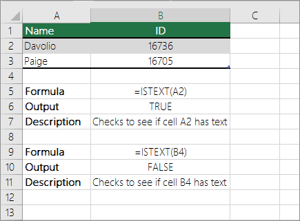
Check if a cell matches specific text
Use the IF function to return results for the condition that you specify.
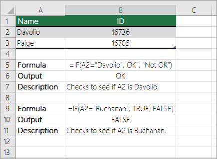
Check if part of a cell matches specific text
To do this task, use the IF, SEARCH, and ISNUMBER functions.
Note: The SEARCH function is case-insensitive.
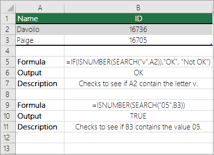
Need more help?
Want more options?
Explore subscription benefits, browse training courses, learn how to secure your device, and more.
Communities help you ask and answer questions, give feedback, and hear from experts with rich knowledge.
This post will guide you how to check if one value in a column exists in another column in Excel. How do I check if value in column A exists in Column B with a formula in Excel. How to determine if values exists in another column in Excel.
Table of Contents
- Check If Value in a Column exists in Another Column
- Related Functions
Assuming that you have a list of data in two columns in range A1:B5, and you want to check if one value in column A exists in column B, if True, then return true, otherwise, returns False. How to achieve it. You can create a new formula based on the IF function, the ISERROR function and the VLOOKUP function. Like this:
=IF(ISERROR(VLOOKUP(A1,$B$1:$B$5, 1, FALSE)),FALSE,TRUE )
Type this formula into cell C1, and press Enter key in your keyboard, and then drag the autofill handle over other cells to apply this formula to check other cells in Column A.
- Excel IF function
The Excel IF function perform a logical test to return one value if the condition is TRUE and return another value if the condition is FALSE. The IF function is a build-in function in Microsoft Excel and it is categorized as a Logical Function.The syntax of the IF function is as below:= IF (condition, [true_value], [false_value])…. - Excel VLOOKUP function
The Excel VLOOKUP function lookup a value in the first column of the table and return the value in the same row based on index_num position.The syntax of the VLOOKUP function is as below:= VLOOKUP (lookup_value, table_array, column_index_num,[range_lookup])…. - Excel ISERROR function
The Excel ISERROR function used to check for any error type that excel generates and it returns TRUE for any error type, and the ISERR function also can be checked for error values except #N/A error, it returns TRUE while the error is #N/A. The syntax of the ISERROR function is as below:= ISERROR (value)….
In this example, the goal is to use a formula to check if a specific value exists in a range. The easiest way to do this is to use the COUNTIF function to count occurences of a value in a range, then use the count to create a final result.
COUNTIF function
The COUNTIF function counts cells that meet supplied criteria. The generic syntax looks like this:
=COUNTIF(range,criteria)Range is the range of cells to test, and criteria is a condition that should be tested. COUNTIF returns the number of cells in range that meet the condition defined by criteria. If no cells meet criteria, COUNTIF returns zero. In the example shown, we can use COUNTIF to count the values we are looking for like this
COUNTIF(data,E5)Once the named range data (B5:B16) and cell E5 have been evaluated, we have:
=COUNTIF(data,E5)
=COUNTIF(B5:B16,"Blue")
=1
COUNTIF returns 1 because «Blue» occurs in the range B5:B16 once. Next, we use the greater than operator (>) to run a simple test to force a TRUE or FALSE result:
=COUNTIF(data,B5)>0 // returns TRUE or FALSEBy itself, the formula above will return TRUE or FALSE. The last part of the problem is to return a «Yes» or «No» result. To handle this, we nest the formula above into the IF function like this:
=IF(COUNTIF(data,E5)>0,"Yes","No")This is the formula shown in the worksheet above. As the formula is copied down, COUNTIF returns a count of the value in column E. If the count is greater than zero, the IF function returns «Yes». If the count is zero, IF returns «No».
Slightly abbreviated
It is possible to shorten this formula slightly and get the same result like this:
=IF(COUNTIF(data,E5),"Yes","No")Here, we have remove the «>0» test. Instead, we simply return the count to IF as the logical_test. This works because Excel will treat any non-zero number as TRUE when the number is evaluated as a Boolean.
Testing for a partial match
To test a range to see if it contains a substring (a partial match), you can add a wildcard to the formula. For example, if you have a value to look for in cell C1, and you want to check the range A1:A100 for partial matches, you can configure COUNTIF to look for the value in C1 anywhere in a cell by concatenating asterisks on both sides:
=COUNTIF(A1:A100,"*"&C1&"*")>0
The asterisk (*) is a wildcard for one or more characters. By concatenating asterisks before and after the value in C1, the formula will count the text in C1 anywhere it appears in each cell of the range. To return «Yes» or «No», nest the formula inside the IF function as above.
An alternative formula using MATCH
As an alternative, you can use a formula that uses the MATCH function with the ISNUMBER function instead of COUNTIF:
=ISNUMBER(MATCH(value,range,0))
The MATCH function returns the position of a match (as a number) if found, and #N/A if not found. By wrapping MATCH inside ISNUMBER, the final result will be TRUE when MATCH finds a match and FALSE when MATCH returns #N/A.
One quick and dirty way to do it is with =COUNTIF(). If the value is found, return the value from cell A1, B1, C1, etc. by filling the formula to the right.
In Sheet 3, Cell A1, enter the following:
=IF(COUNTIF(Sheet2!$A:$A,Sheet1!$A1),Sheet1!A1)
Now use the Fill right (Ctrl+R) and Fill down (Ctrl+D) features to apply the formula to as many cells as required, depending on the number of columns+rows expected in the raw data you have in Sheet 1. If the search is successful, it will fill out the data from that row in Sheet 1.
If the search is unsuccessful, the row will return FALSE. If a cell on sheet 1 does not have data, it will return 0. If desired, you can return blank text («») instead of a FALSE or a 0 with a formula like:
=IF(COUNTIF(Sheet2!$A:$A,Sheet1!$A1),IF(ISBLANK(Sheet1!A1),"",Sheet1!A1),"")
To say it again — this is quick and dirty and will have performance implications if you have a large dataset. You are typically better off putting your raw data in a database — you can then use a Pivot Table or simple SQL queries to extract the data you need in the format required.
Excel has a number of formulas that help you use your data in useful ways. For example, you can get an output based on whether or not a cell meets certain specifications. Right now, we’ll focus on a function called “if cell contains, then”. Let’s look at an example.
Jump To Specific Section:
- Explanation: If Cell Contains
- If cell contains any value, then return a value
- If cell contains text/number, then return a value
- If cell contains specific text, then return a value
- If cell contains specific text, then return a value (case-sensitive)
- If cell does not contain specific text, then return a value
- If cell contains one of many text strings, then return a value
- If cell contains several of many text strings, then return a value
Excel Formula: If cell contains
Generic formula
=IF(ISNUMBER(SEARCH("abc",A1)),A1,"")
Summary
To test for cells that contain certain text, you can use a formula that uses the IF function together with the SEARCH and ISNUMBER functions. In the example shown, the formula in C5 is:
=IF(ISNUMBER(SEARCH("abc",B5)),B5,"")
If you want to check whether or not the A1 cell contains the text “Example”, you can run a formula that will output “Yes” or “No” in the B1 cell. There are a number of different ways you can put these formulas to use. At the time of writing, Excel is able to return the following variations:
- If cell contains any value
- If cell contains text
- If cell contains number
- If cell contains specific text
- If cell contains certain text string
- If cell contains one of many text strings
- If cell contains several strings
Using these scenarios, you’re able to check if a cell contains text, value, and more.
Explanation: If Cell Contains
One limitation of the IF function is that it does not support Excel wildcards like «?» and «*». This simply means you can’t use IF by itself to test for text that may appear anywhere in a cell.
One solution is a formula that uses the IF function together with the SEARCH and ISNUMBER functions. For example, if you have a list of email addresses, and want to extract those that contain «ABC», the formula to use is this:
=IF(ISNUMBER(SEARCH("abc",B5)),B5,""). Assuming cells run to B5
If «abc» is found anywhere in a cell B5, IF will return that value. If not, IF will return an empty string («»). This formula’s logical test is this bit:
ISNUMBER(SEARCH("abc",B5))
Read article: Excel efficiency: 11 Excel Formulas To Increase Your Productivity
Using “if cell contains” formulas in Excel
The guides below were written using the latest Microsoft Excel 2019 for Windows 10. Some steps may vary if you’re using a different version or platform. Contact our experts if you need any further assistance.
1. If cell contains any value, then return a value
This scenario allows you to return values based on whether or not a cell contains any value at all. For example, we’ll be checking whether or not the A1 cell is blank or not, and then return a value depending on the result.
- Select the output cell, and use the following formula: =IF(cell<>»», value_to_return, «»).
- For our example, the cell we want to check is A2, and the return value will be No. In this scenario, you’d change the formula to =IF(A2<>»», «No», «»).
- Since the A2 cell isn’t blank, the formula will return “No” in the output cell. If the cell you’re checking is blank, the output cell will also remain blank.
2. If cell contains text/number, then return a value
With the formula below, you can return a specific value if the target cell contains any text or number. The formula will ignore the opposite data types.
Check for text
- To check if a cell contains text, select the output cell, and use the following formula: =IF(ISTEXT(cell), value_to_return, «»).
- For our example, the cell we want to check is A2, and the return value will be Yes. In this scenario, you’d change the formula to =IF(ISTEXT(A2), «Yes», «»).

- Because the A2 cell does contain text and not a number or date, the formula will return “Yes” into the output cell.
Check for a number or date
- To check if a cell contains a number or date, select the output cell, and use the following formula: =IF(ISNUMBER(cell), value_to_return, «»).
- For our example, the cell we want to check is D2, and the return value will be Yes. In this scenario, you’d change the formula to =IF(ISNUMBER(D2), «Yes», «»).

- Because the D2 cell does contain a number and not text, the formula will return “Yes” into the output cell.
3. If cell contains specific text, then return a value
To find a cell that contains specific text, use the formula below.
- Select the output cell, and use the following formula: =IF(cell=»text», value_to_return, «»).
- For our example, the cell we want to check is A2, the text we’re looking for is “example”, and the return value will be Yes. In this scenario, you’d change the formula to =IF(A2=»example», «Yes», «»).

- Because the A2 cell does consist of the text “example”, the formula will return “Yes” into the output cell.
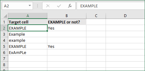
4. If cell contains specific text, then return a value (case-sensitive)
To find a cell that contains specific text, use the formula below. This version is case-sensitive, meaning that only cells with an exact match will return the specified value.
- Select the output cell, and use the following formula: =IF(EXACT(cell,»case_sensitive_text»), «value_to_return», «»).
- For our example, the cell we want to check is A2, the text we’re looking for is “EXAMPLE”, and the return value will be Yes. In this scenario, you’d change the formula to =IF(EXACT(A2,»EXAMPLE»), «Yes», «»).
- Because the A2 cell does consist of the text “EXAMPLE” with the matching case, the formula will return “Yes” into the output cell.
5. If cell does not contain specific text, then return a value
The opposite version of the previous section. If you want to find cells that don’t contain a specific text, use this formula.
- Select the output cell, and use the following formula: =IF(cell=»text», «», «value_to_return»).
- For our example, the cell we want to check is A2, the text we’re looking for is “example”, and the return value will be No. In this scenario, you’d change the formula to =IF(A2=»example», «», «No»).
- Because the A2 cell does consist of the text “example”, the formula will return a blank cell. On the other hand, other cells return “No” into the output cell.
6. If cell contains one of many text strings, then return a value
This formula should be used if you’re looking to identify cells that contain at least one of many words you’re searching for.
- Select the output cell, and use the following formula: =IF(OR(ISNUMBER(SEARCH(«string1», cell)), ISNUMBER(SEARCH(«string2», cell))), value_to_return, «»).
- For our example, the cell we want to check is A2. We’re looking for either “tshirt” or “hoodie”, and the return value will be Valid. In this scenario, you’d change the formula to =IF(OR(ISNUMBER(SEARCH(«tshirt»,A2)),ISNUMBER(SEARCH(«hoodie»,A2))),»Valid «,»»).
- Because the A2 cell does contain one of the text values we searched for, the formula will return “Valid” into the output cell.
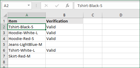
To extend the formula to more search terms, simply modify it by adding more strings using ISNUMBER(SEARCH(«string», cell)).
7. If cell contains several of many text strings, then return a value
This formula should be used if you’re looking to identify cells that contain several of the many words you’re searching for. For example, if you’re searching for two terms, the cell needs to contain both of them in order to be validated.
- Select the output cell, and use the following formula: =IF(AND(ISNUMBER(SEARCH(«string1»,cell)), ISNUMBER(SEARCH(«string2″,cell))), value_to_return,»»).
- For our example, the cell we want to check is A2. We’re looking for “hoodie” and “black”, and the return value will be Valid. In this scenario, you’d change the formula to =IF(AND(ISNUMBER(SEARCH(«hoodie»,A2)),ISNUMBER(SEARCH(«black»,A2))),»Valid «,»»).
- Because the A2 cell does contain both of the text values we searched for, the formula will return “Valid” to the output cell.
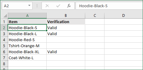
Final thoughts
We hope this article was useful to you in learning how to use “if cell contains” formulas in Microsoft Excel. Now, you can check if any cells contain values, text, numbers, and more. This allows you to navigate, manipulate and analyze your data efficiently.
We’re glad you’re read the article up to here  Thank you
You may also like
» How to use NPER Function in Excel
» How to Separate First and Last Name in Excel
» How to Calculate Break-Even Analysis in Excel