Excel if value in cell is in a range

In this example, the goal is to use a formula to check if a specific value exists in a range. The easiest way to do this is to use the COUNTIF function to count occurences of a value in a range, then use the count to create a final result.

COUNTIF function

The COUNTIF function counts cells that meet supplied criteria. The generic syntax looks like this:

=COUNTIF(range,criteria)

Range is the range of cells to test, and criteria is a condition that should be tested. COUNTIF returns the number of cells in range that meet the condition defined by criteria. If no cells meet criteria, COUNTIF returns zero. In the example shown, we can use COUNTIF to count the values we are looking for like this

COUNTIF(data,E5)

Once the named range data (B5:B16) and cell E5 have been evaluated, we have:

=COUNTIF(data,E5)
=COUNTIF(B5:B16,"Blue")
=1

COUNTIF returns 1 because «Blue» occurs in the range B5:B16 once. Next, we use the greater than operator (>) to run a simple test to force a TRUE or FALSE result:

=COUNTIF(data,B5)>0 // returns TRUE or FALSE

By itself, the formula above will return TRUE or FALSE. The last part of the problem is to return a «Yes» or «No» result. To handle this, we nest the formula above into the IF function like this:

=IF(COUNTIF(data,E5)>0,"Yes","No")

This is the formula shown in the worksheet above. As the formula is copied down, COUNTIF returns a count of the value in column E. If the count is greater than zero, the IF function returns «Yes». If the count is zero, IF returns «No».

Slightly abbreviated

It is possible to shorten this formula slightly and get the same result like this:

=IF(COUNTIF(data,E5),"Yes","No")

Here, we have remove the «>0» test. Instead, we simply return the count to IF as the logical_test. This works because Excel will treat any non-zero number as TRUE when the number is evaluated as a Boolean.

Testing for a partial match

To test a range to see if it contains a substring (a partial match), you can add a wildcard to the formula. For example, if you have a value to look for in cell C1, and you want to check the range A1:A100 for partial matches, you can configure COUNTIF to look for the value in C1 anywhere in a cell by concatenating asterisks on both sides:

=COUNTIF(A1:A100,"*"&C1&"*")>0

The asterisk (*) is a wildcard for one or more characters. By concatenating asterisks before and after the value in C1, the formula will count the text in C1 anywhere it appears in each cell of the range. To return «Yes» or «No», nest the formula inside the IF function as above.

An alternative formula using MATCH

As an alternative, you can use a formula that uses the MATCH function with the ISNUMBER function instead of COUNTIF:

=ISNUMBER(MATCH(value,range,0))

The MATCH function returns the position of a match (as a number) if found, and #N/A if not found. By wrapping MATCH inside ISNUMBER, the final result will be TRUE when MATCH finds a match and FALSE when MATCH returns #N/A.

Home / Excel Formulas / Check IF a Value Exists in a Range

In Excel, to check if a value exists in a range or not, you can use the COUNTIF function, with the IF function. With COUNTIF you can check for the value and with IF, you can return a result value to show to the user. i.e., Yes or No, Found or Not Found.

In the following example, you have a list of names where you only have first names, and now, you need to check if “Arlene” is there or not.

You can use the following steps:

1. First, you need to enter the IF function in cell B1.
   
2. After that, in the first argument (logical test), you need to enter the COUNTIF function there.
   
3. Now, in the COUNTIF function, refer to the range A1:A10.
   
4. Next, in the criteria argument, enter “Glen” and close the parentheses for the COUNTIF Function.
   
5. Additionally, use a greater than sign and enter a zero.
   
6. From here, enter a comma to go to the next argument in the IF, and enter “Yes” in the second argument.
   
7. In the end, enter a comma and enter “No” in the third argument and type the closing parentheses.
   

The moment you hit enter it returns “Yes”, as you have the value in the range that you have searched for.

=IF(COUNTIF(A1:A10,"Glen")>0,"Yes","No")

How this Formula Works

This formula has two parts.

In the first part, we have COUNTIF, which counts the occurrence of the value in the range. And in the second part, you have the IF function that takes the values from the COUNTIF function.

So, if COUNTIF returns any value greater than which means the value is there in the range IF returns Yes. And if COUNTIF returns 0, which means the value is not there in the range and it returns No.

Check for a Value in a Range Partially

There counts to be a situation where you want to check for partial value from a range. In that case, you need to use wildcard characters (asterisk *).

In the following example, we have the same list of names but here is the full name. But we still need to look for the name “Glen”.

=IF(COUNTIF(C1:C10,"*"&"Glen"&"*")>0,"Yes","No")

The value you want to search for needs to be enclosed with an asterisk, which we have used in the above example. This tells Excel, to check for the value “Glen” regardless of what is there before and after the value.

And, if you want to Get Smarter than Your Colleagues check out these FREE COURSES to Learn Excel, Excel Skills, and Excel Tips and Tricks.

Author: Oscar Cronquist Article last updated on February 17, 2023

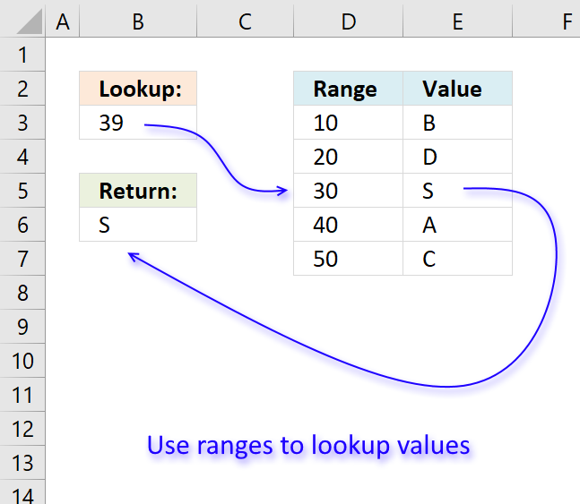
In this article, I will demonstrate four different formulas that allow you to lookup a value that is to be found in a given range and return the corresponding value on the same row. If you need to return multiple values because the ranges overlap then read this article: Return multiple values if in range.

They all have their pros and cons and I will discuss those in great detail, they can be applied to not only numerical ranges but also text ranges and date ranges as well.

I have made a video that explains the LOOKUP function in context to this article, if you are interested.

There is a file for you to get, at the end of this article, which contains all the formula examples in a worksheet each.

You can use the techniques described in this article to calculate discount percentages based on price intervals or linear results based on the lookup value.

Check out the LOOKUP category to find more interesting articles.

The following table shows the differences between the formulas presented in this article.

Formula	Range sorted?	Array formula	Get value from any column?	Two range columns?
LOOKUP	Yes	No	Yes	No
INDEX + SUMPRODUCT + ROW	No	No	Yes	Yes
VLOOKUP	Yes	No	No	No
INDEX + MATCH	Yes	No	Yes	No

Some formulas require you to have the lookup range sorted to function properly, the INDEX+SUMPRODUCT+ROW alternative is the only way to go if you can’t sort the values.

The disadvantage with the INDEX+SUMPRODUCT+ROW formula is that you need start and end values, the other formulas use the start values also as end range values.

The VLOOKUP function can only search the leftmost column, you must rearrange your table to meet this condition if you are going to use the VLOOKUP function.

1. If value in range then return value — LOOKUP function

To better demonstrate the LOOKUP function I am going to answer the following question.

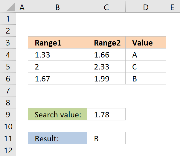
The next image shows the table in greater detail.

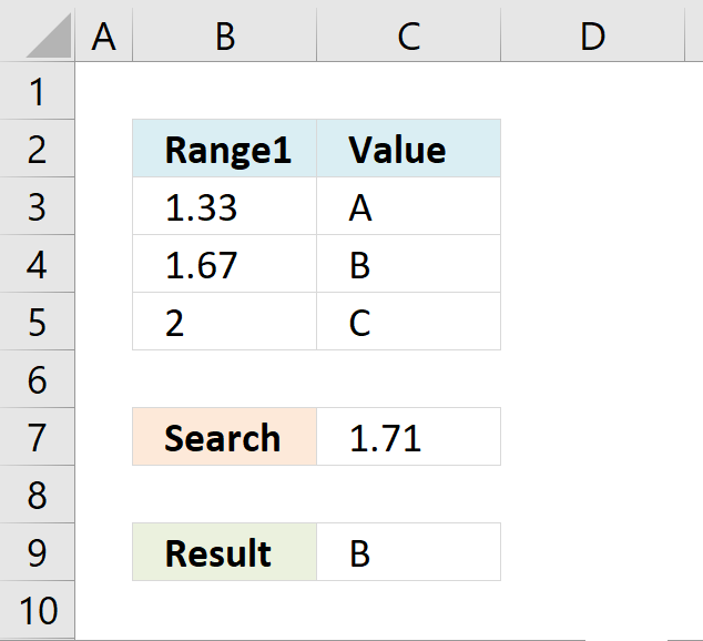
The picture above shows data in cell range B3:C5, the search value is in C7 and the result is in C9.

Cell range B3:B5 must be sorted in ascending order for the LOOKUP function to work properly.

Ascending order means values are sorted from the smallest to the largest value. Example: 1,5,8,11.

If an exact match is not found the largest value is returned as long as it is smaller than the lookup value.

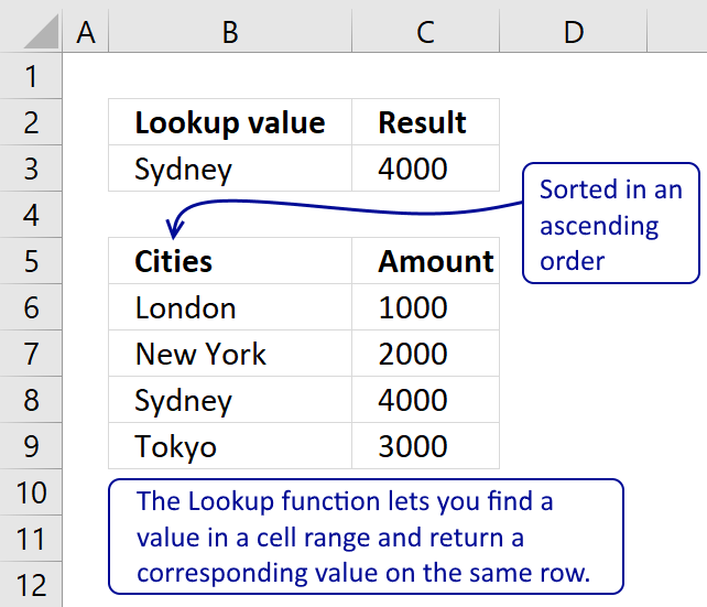
The LOOKUP function then returns a value in a column on the same row.

The formula in cell C9:

=LOOKUP(C8,B4:B6,C4:C6)

Example, Search value 1.71 has no exact match, the largest value that is smaller than 1.71 is 1.67. The returning value is found in column C on the same row as 1.67, in this case, B.

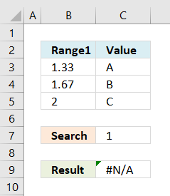If the search value is smaller than the smallest value in the lookup range the function returns #N/A meaning Not Available or does not exist.

Example in the picture to the right, search value is 1 in the and the LOOKUP function returns #N/A.

To solve this problem simply add another number, for example 0. Cell range B3:B6 would then contain 0, 1.33, 1.67, 2.

A search value greater than the largest value in the lookup range matches the largest value. Example in above picture, search value is 3 and the returning value is C.

Watch video below to see how the LOOKUP function works:

Learn more about the LOOKUP function, recommended reading:

Recommended articles

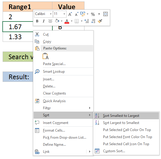
Tip! — You can quickly sort a cell range, follow these steps:

1. Press with right mouse button on on a cell in the cell range you want to sort
   
2. Hover with mouse cursor over Sort
3. Press with mouse on «Sort Smallest to Largest»

Back to top

2. If the value is in the range then return value — INDEX + SUMPRODUCT + ROW

The following formula is slightly larger but you don’t need to sort cell range B4:B6.

The formula in cell C11:

=INDEX(D4:D6, SUMPRODUCT(—($D$8<=C4:C6), —($D$8>=B4:B6), ROW(A1:A3)))

The ranges don’t need to be sorted however you need a start (Range1) and an end value (Range2).

Back to top

Explaining formula in cell C11

You can easily follow along, go to tab «Formulas» and press with left mouse button on «Evaluate Formula» button. Press with left mouse button on «Evaluate» button to move to next step.

Step 1 — Calculate first condition

The bolded part is the the logical expression I am going to explain in this step.

=INDEX(D4:D6, SUMPRODUCT(—($D$8<=C4:C6), —($D$8>=B4:B6), ROW(A1:A3)))

The gretaer than sign combined with the equal sign <= means if value in cell D8 is smaller than or equal to the values in cell range C4:C6.

—($D$8<=C4:C6)

becomes

—(1,78<={1,66;1,99;2,33})

becomes

—{1,78<=1,66; 1,78<=1,99; 1,78<=2,33})

becomes

—({FALSE;TRUE;TRUE})

and returns {0;1;1}.

The double minus signs convert the boolean value TRUE or FALSE to the corresponding number 1 or 0 (zero).

Step 2 — Calculate second criterion

=INDEX(D4:D6, SUMPRODUCT(—($D$8<=C4:C6), —($D$8>=B4:B6), ROW(A1:A3)))

—($D$8>=B4:B6)

becomes

—(1,78>={1,33;1,67;2})

becomes

—({TRUE;TRUE;FALSE})

and returns

{1;1;0}

Step 3 — Create row numbers

=INDEX(D4:D6, SUMPRODUCT(—($D$8<=C4:C6), —($D$8>=B4:B6), ROW(A1:A3)))

ROW(A1:A3)

returns

{1;2;3}

Step 4 — Multiply criteria and row numbers and sum values

=INDEX(D4:D6, SUMPRODUCT(—($D$8<=C4:C6), —($D$8>=B4:B6), ROW(A1:A3)))

SUMPRODUCT(—($D$8<=C4:C6), —($D$8>=B4:B6), ROW(A1:A3))

becomes

SUMPRODUCT({0;1;1}, {1;1;0}, {1;2;3})

becomes

SUMPRODUCT({0;2;0})

and returns number 2.

Step 5 — Return a value of the cell at the intersection of a particular row and column

=INDEX(D4:D6, SUMPRODUCT(—($D$8<=C4:C6), —($D$8>=B4:B6), ROW(A1:A3)))

becomes

=INDEX(D4:D6, 2)

becomes

=INDEX({«A»;»B»;»C»}, 2)

and returns «B».

Functions in this formula: INDEX, SUMPRODUCT, ROW

Back to top

3. If value in range then return value — VLOOKUP function

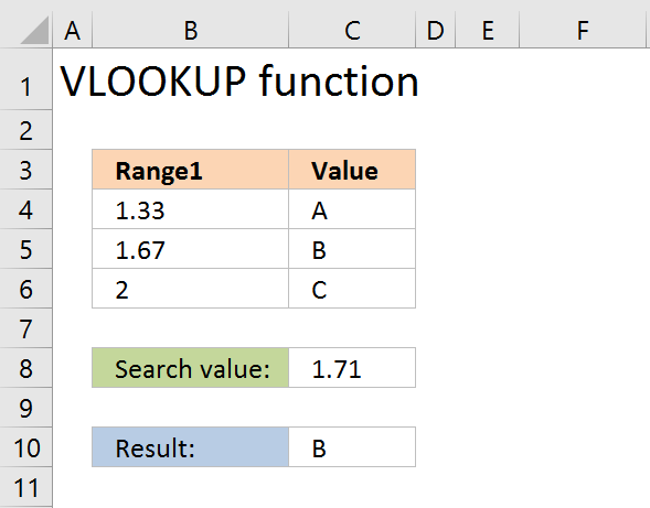
=VLOOKUP($D$8,$B$4:$D$6,3,TRUE)

The VLOOKUP function requires the table to be sorted based on range1 in an ascending order.

Back to top

Explaining the VLOOKUP formula in cell C10

The VLOOKUP function looks for a value in the leftmost column of a table and then returns a value in the same row from a column you specify.

Arguments:
VLOOKUP(
lookup_value,
table_array,
col_index_num, [range_lookup]
)

The [range_lookup] argument is important in this case, it determines how the VLOOKUP function matches the lookup_value in the table_array.

The [range_lookup] is optional, it is either TRUE (default) or FALSE. It must be TRUE in our example here so that VLOOKUP returns an approximate match.

In order to do an approximate match the table_array must be sorted in an ascending order based on the first column.

=VLOOKUP($D$8,$B$4:$D$6,3,TRUE)

becomes

=VLOOKUP(1,78,{1,33, 1,66, «A»;1,67, 1,99, «B»;2, 2,33, «C»},3,TRUE)

1,67 is the next largest value and the VLOOKUP function returns «B».

Back to top

4. If value in range then return value — INDEX + MATCH

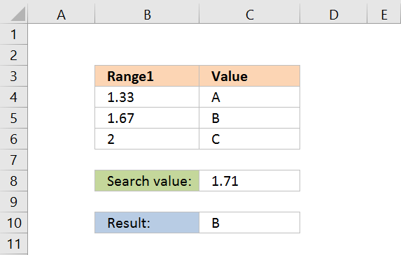
Formula in cell C10:

=INDEX($D$4:$D$6,MATCH(D8,$B$4:$B$6,1))

The lookup range must be sorted, just like the LOOKUP and VLOOKUP functions. Functions in this formula: INDEX and MATCH

Thanks JP!

Back to top

Explaining INDEX+MATCH in cell D10

=INDEX($D$4:$D$6,MATCH(D8,$B$4:$B$6,1))

Step 1 — Return the relative position of an item in an array

The MATCH function returns the relative position of an item in an array or cell range that matches a specified value

Arguments:
MATCH(
lookup_value,
lookup_array,
[match_type])
)

The [match_type] argument is optional. It can be either -1, 0, or 1. 1 is default value if omitted.

The match_type argument determines how the MATCH function matches the lookup_value with values in lookup_array.

We want it to do an approximate search so I am going to use 1 as the argument.

This will make the MATCH find the largest value that is less than or equal to lookup_value. However, the values in the lookup_array argument must be sorted in an ascending order.

To learn more about the [match_type] argument read the article about the MATCH function.

=INDEX($D$4:$D$6,MATCH(D8,$B$4:$B$6,1))

MATCH(D8,$B$4:$B$6,1)

becomes

MATCH(1.78,{1.33;1.67;2},1)

1.67 is the largest value that is less than or equal to lookup_value. 1.67 is the second value in the array. MATCH function returns 2.

Step 2 — Return a value of the cell at the intersection of a particular row and column

=INDEX($D$4:$D$6,MATCH(D8,$B$4:$B$6,1))

becomes

=INDEX($D$4:$D$6,2)

becomes

=INDEX({«A»;»B»;»C»},2)

and returns «B».

Back to top

Back to top

Quickly lookup a value in a numerical range

You can also do lookups in date ranges, dates in Excel are actually numbers.

In this article, we will learn Find if a character is in a range and cell in Microsoft Excel.

Scenario:

In simple words, while working with data tables, sometimes we need to get the sum of the cells where ranges meet one or more text values having OR criteria. For example finding the count of values in a range matching particular ID Or finding the sum of quantity for a particular product in the table.Criteria is the value in range that can match with one or more required values given in another list.

How to solve the problem?

For this article we will be required to use the SUMPRODUCT function. Now we will make a formula out of these functions. Here we are given a dataset and a range and we need to match either of the values in range and get the sum of corresponding values from dataset.

Generic formula:

range : range to match with criteria range

cri_range : criteria range

sum_range : range where sum is required

Example :

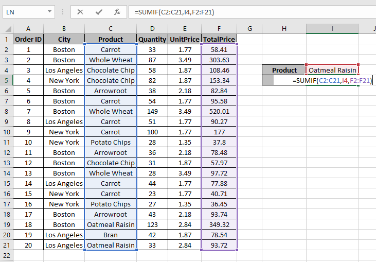
All of these might be confusing to understand. Let’s understand how to use the function using an example. Here we have Order IDs from different regions with their respective quantity and Price.

We need to get the sum of TotalPrice for a specific Product in other cell I4.

Use the formula:

=SUMIF(C2:C21, I4, F2:F21)

Explanation:

C2:C21 : range where formula matches values.

 I4 : Value from the other cell to match with C2:C21 range

A2:A26 : sum_range where amount adds up.

=SUMIF({"Carrot";"Whole Wheat";"Chocolate Chip";"Chocolate Chip";"Arrowroot";"Carrot";"Whole Wheat";"Carrot";"Carrot";"Potato Chips";"Arrowroot";"Chocolate Chip";"Whole Wheat";"Carrot";"Carrot";"Potato Chips";"Arrowroot";"Oatmeal Raisin";"Bran";"Oatmeal Raisin"},
I4,
{58.41;303.63;108.46;153.34;82.84;95.58;520.01;90.27;177;37.8;78.48;57.97;97.72;77.88;40.71;36.45;93.74;349.32;78.54;93.72})

This formula adds up all the values corresponding to all the values in cell I4 i.e. “Oatmeal raisin

Press Enter to get the Sum

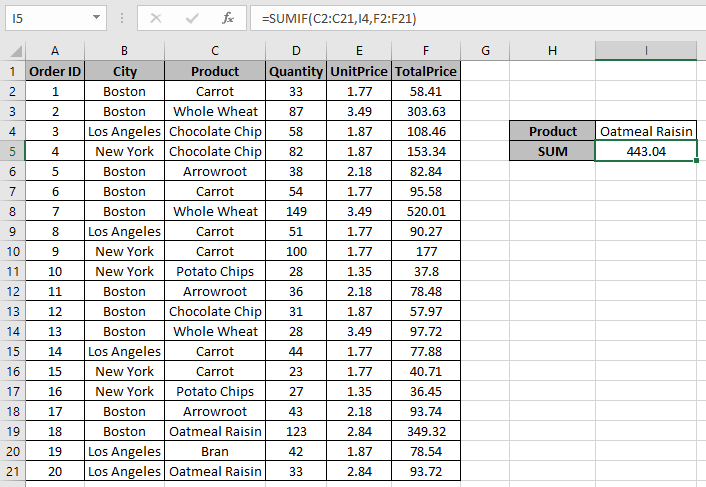
The formula returns 443.04 as the sum for the value in the other cell.

As you can see this formula returns the sum if the cell is equal to a value.

Another Example:

Here we have a dataset (A1:D50) having the order date, city, product & its quantity.

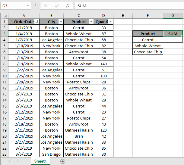
Firstly,  we need to find the sum of quantity where the product matches any of the values mentioned in the separate range. Now we will use the following formula to get the sum

Use the Formula:

E5:E11 : range in dataset which needs to be matched

product : criteria range

D2:D50 : sum range, sum of quantity

Explanation:

• SUMIF function returns the sum if it has to match one value with the range. But here SUMIF takes the argument and returns an array to SUMPRODUCT function.

=SUMPRODUCT ( { 760 ; 348 ; 499 } )

• SUMPRODUCT function gets the returned array, which has an array of sum of quantity for different products and returns the SUM of the returned array.

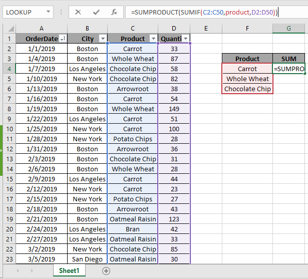
Here the range is given as cell reference and criteria range is given as named range. Press Enter to get the count.

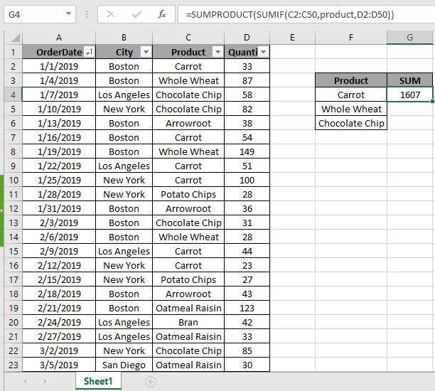
As you can see in the above snapshot that sum of quantity having carrot, chocolate chip or whole wheat is 1607.

Here are some observational notes shown below.

Notes:

1. The formula only works with numbers.
2. The formula works only when there are no duplicates in the lookup table
3. The SUMPRODUCT function considers non — numeric values as 0s.
4. The SUMPRODUCT function considers logic value TRUE as 1 and False as 0.
5. The argument array must be of the same length else the function.

Hope this article about Find if a character is in a range and cell in Microsoft Excel is explanatory. Find more articles on calculating values and related Excel formulas here. If you liked our blogs, share it with your friends on Facebook. And also you can follow us on Twitter and Facebook. We would love to hear from you, do let us know how we can improve, complement or innovate our work and make it better for you. Write to us at info@exceltip.com.

Related Articles :

How to use the SUMPRODUCT function in Excel: Returns the SUM after multiplication of values in multiple arrays in excel.

SUM if date is between : Returns the SUM of values between given dates or period in excel.

Sum if date is greater than given date: Returns the SUM of values after the given date or period in excel.

2 Ways to Sum by Month in Excel: Returns the SUM of values within a given specific month in excel.

How to Sum Multiple Columns with Condition: Returns the SUM of values across multiple columns having condition in excel

How to use wildcards in excel : Count cells matching phrases using the wildcards in excel

Popular Articles :

How to use the IF Function in Excel : The IF statement in Excel checks the condition and returns a specific value if the condition is TRUE or returns another specific value if FALSE.

How to use the VLOOKUP Function in Excel : This is one of the most used and popular functions of excel that is used to lookup value from different ranges and sheets.

How to use the SUMIF Function in Excel : This is another dashboard essential function. This helps you sum up values on specific conditions.

How to use the COUNTIF Function in Excel : Count values with conditions using this amazing function. You don’t need to filter your data to count specific values. Countif function is essential to prepare your dashboard.

EXPLANATION

This tutorial shows how to test if a range contains a specific value and return a specified value if the formula tests true or false, by using an Excel formula and VBA.

This tutorial provides one Excel method that can be applied to test if a range contains a specific value and return a specified value by using an Excel IF and COUNTIF functions. In this example, if the Excel COUNTIF function returns a value greater than 0, meaning the range has cells with a value of 500, the test is TRUE and the formula will return a «In Range» value. Alternatively, if the Excel COUNTIF function returns a value of of 0, meaning the range does not have cells with a value of 500, the test is FALSE and the formula will return a «Not in Range» value.

This tutorial provides one VBA method that can be applied to test if a range contains a specific value and return a specified value.

FORMULA
=IF(COUNTIF(range, value)>0, value_if_true, value_if_false)

ARGUMENTS
range: The range of cells you want to count from.
value: The value that is used to determine which of the cells should be counted, from a specified range, if the cells’ value is equal to this value.
value_if_true: Value to be returned if the range contains the specific value
value_if_false: Value to be returned if the range does not contains the specific value.

Find if a cell or range of cells contains a specific value in Excel. This method can be used on individual cells when you want to «mark» them or to find out how many cells in a range contain that specific value.

With this method, it doesn’t matter where the text, number, or value is located within the cell.

Sections:

Find if a Value is Contained in a Specific Cell

Find if a Value is in a Range of Cells

Find a Value that is Separate from Other Text in a Cell

Notes

Find if a Value is Contained in a Specific Cell

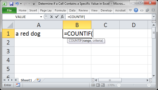
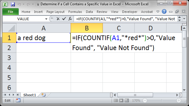
Let’s find out if the word red is in cell A1.

1. Go to an empty cell and type =COUNTIF(
   
   
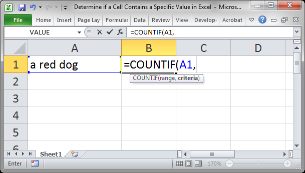
2. Select cell A1, the cell with the text, and then type a comma so we can move to the next argument in Step 3.
   
3. Type «*red*»
   
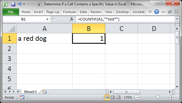
   Notice the symbol * around the text. This is what tells the function to look for the word red anywhere inside the cell. You must put this symbol at the start and end of the value for which you are searching.
   Also, note that everything is encapsulated inside of double quotes «». You must surround everything, including the * symbol with double quotation marks, as in the example.
4. Type a closing parenthesis ) and then hit Enter.
   
   You see 1 in the cell because the COUNTIF function counts how many times it found a value in a cell and it found the value red once in cell A1. If it did not find the value it would return a zero 0.
   We use this technique to determine if the value is in the cell. In our example here it doesn’t matter how many times the value is in the cell, only that it is there.
5. That’s it!

You can stop here and use this output any way you like, or you can add a more visual representation of this data by surrounding the COUNTIF function with an IF statement and doing something like this:

The output will be like this:

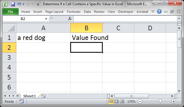
Here is the final code with the IF statement included:

Here is the code without the IF statement:

Find if a Value is in a Range of Cells

This is almost exactly the same as the previous example except that we want to look through a range of cells to determine if the value is located there.

This method will also count how many times the desired value appears within the range.

To do this, follow the steps from the previous example, but, for Step 2, select a range of cells instead of just a single cell.

It will look like this:

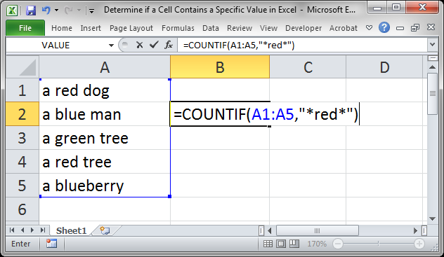
With a result like this:

This means that the text red was found twice in the range of cells.

The COUNTIF function won’t tell you the location of the cells with the text; it will only tell you that the text is present in the range and how many times it appears.

For a more detailed explanation of how this works, look to the previous example (the first example) in this tutorial.

Find a Value that is Separate from Other Text in a Cell

This tutorial assumes that you are looking for a distinct value within a cell or range of cells and the above methods work well 95% of the time. However, those methods will also return values that are part of other values.

So, if I want to check if the word red appears in a cell using the above method but there are some cells where red is a part of a larger word, Excel will still count that as having found the word red, which is not what we want.

If your data might be setup like this, then we need to specify that we want to find only the whole word red. Since words are surrounded by spaces, we alter the initial formula to be like this:

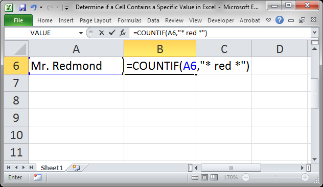
Notice the spaces between the * symbols and the value red. This means that the word red will only be found/counted if it has a space to the left and right of it within the cell, which makes it a word instead of a part of a word.

In this example, it won’t find red in cell A6:

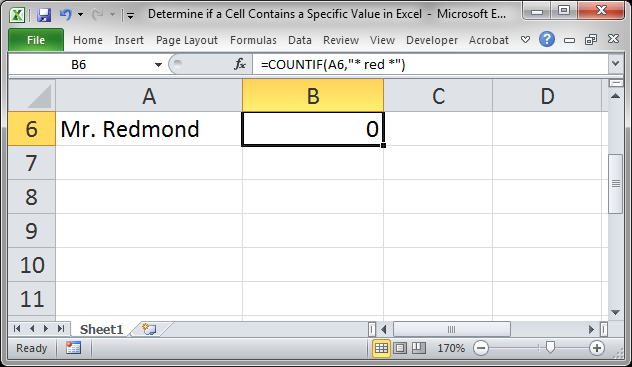
The original formula would have counted the red in Redmond as 1.

In my data spaces worked fine, but you may need to use different characters to surround your text depending on that for which you are searching.

Notes

There are other ways to do this, including using the FIND function, but I have found that the COUNTIF function works well, is a bit more versatile, and is easier for most people to understand and use.

This tutorial shows you a neat little way to use a counting function to determine if a cell contains a specific value or not. I hope this will help you to start thinking of creative ways to solve your Excel issues.

This method is not case sensitive.

Make sure to download the attached spreadsheet so you can work with these examples in Excel.

Similar Content on TeachExcel

Subscribe for Weekly Tutorials

BONUS: subscribe now to download our Top Tutorials Ebook!

Return to Excel Formulas List

In this tutorial you will learn how to test if a range contains a specific value.

In this Article

• COUNTIF Function
• Example: Countif Cells Contain Certain Text
• Alternative Expressions for the formula used
• Manipulating the COUNTIF Function
• COUNTIFS Function with Multiple Criteria
• EXAMPLE

COUNTIF Function

In Excel, the COUNTIF function is used to determine if a value exists in a range of cells. The general formula for the COUNTIF is as follows:

=COUNTIF(range, criteria)

Range is the group of cells that you want to count. They can contain numbers, arrays, be named, or have references that contain numbers.

Criteria is a number (5), expression (>5), cell reference (A9), or word (Knights) that determines which cells to count.

We will use the COUNTIF function to solve the following example.

Example: Countif Cells Contain Certain Text

Suppose a school wants to change their team mascot. They give 6 different options to student council officials and decide that only mascots with more than 4 votes will be considered. What mascots will the school consider?

Part 1) First we have to have to determine how many votes each mascot got. To do so we use the following formula:

=COUNTIF(Mascots, A9)

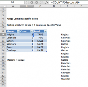
Range E9:E23 was renamed to “Mascots” for simplicity purposes using a Named Range

This will count the number of cells in the list of Mascots that match the value of A9. The result is 5. To quickly fill in the remaining cells you can simply select the cell that you want to use as a basis and drag the fill handle .

Alternative Expressions for the formula used

• =COUNTIF(E9:E23, “Knights”) Will count the number of cells with Knights in cells E9 through E23. The result is 5.
• =COUNTIF(E9:E23, “?nights”) Will count the number of cells that have exactly 7 characters and end with the letters “nights” in cells E9:E23. The question mark (?) acts as a wildcard to replace an individual character. The result is 5.
• =COUNTIF(E9:E23,”<>”&”Knights”) Will count the number of cells in the range E9 through E23 that don’t contain Knights. The result is 10.

Part 2) Next, we have to determine which mascots received more than 4 votes. To do so we will use the COUNTIF function to run a simple TRUE or FALSE test.

=COUNTIF(Mascots, A9)>4

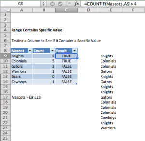
This formula will produce the answer TRUE if the desired mascot appears in the range more than 4 times and FALSE if it appears less than or equal to 4 times. Once again we can select the cell that we want to use as a basis and drag the fill handle  in order to fill the remaining cells.

Manipulating the COUNTIF Function

We can also wrap the formula inside an IF statement in order to produce a result different than TRUE or FALSE.

=IF(COUNTIF(Mascots,A9)>4,”Consider”,”Reject”)

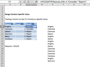
Instead of producing the result TRUE or FALSE, this formula will cause Excel to produce the result Consider or Reject.

COUNTIFS Function with Multiple Criteria

Once you learn how to use the COUNTIF function with one range and criteria, it is easy to use it for two or more range/criteria combinations. When testing if a range contains multiple values we must use the COUNTIFS function.

EXAMPLE

Let’s say we have a list of car parts ordered. We want to count the number of times a car part was ordered for its corresponding vehicle.

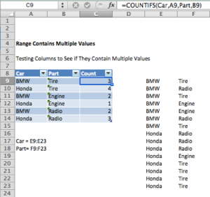
By using the general formula:

=COUNTIFS(range1,criteria1,range2,criteria2)

We are able to determine where both criteria are matched in their respective columns. Let it be noted that the two criteria ranges must be the same shape and size or the formula will not work.