
To control more precisely what cells will be formatted, you can use formulas to apply conditional formatting.
Want more?
Use conditional formatting
Manage conditional formatting rule precedence
To control more precisely what cells will be formatted, you can use formulas to apply conditional formatting.
In this example, I am going to format the cells in the Product column if the corresponding cell in the In stock column is greater than 300.
I select the cells I want to conditionally format.
When you select a range of cells, the first cell you select is the active cell.
In this example, I selected from B2 through B10, so B2 is the active cell. We’ll need to know that shortly.
Create a new rule, select Use a formula to determine which cells to format. Since B2 is the active cell, I type =E2>300.
Note that in the formula, I used the relative cell reference E2 to make sure the formula adjusts to correctly format the other cells in column B.
I click the Format button and choose how I want to format the cells. I am going to use a blue fill.
Click OK to accept the color; click OK again to apply the format.
And the cells in the Product column, where the corresponding cell in column E is greater than 300, are conditionally formatted.
When I change a value in column E to greater than 300, the conditional formatting in the Product column automatically applies.
You can create multiple rules that apply to the same cells.
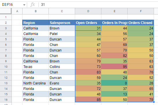
In this example, I want different fill colors for different ranges of scores.
I select the cells I want to apply a rule to, create a new rule that uses the rule type Use a formula to determine which cells to format.
I want to format a cell if its value is greater than or equal to 90.
The active cell is B2, so I enter the formula =B2>=90.
And configure the rule to apply a green fill when the formula is true for a cell. The cell that has a value greater than or equal to 90 is filled with green.
I create another rule for the same cells, but this time, I want to format a cell if its value is greater than or equal to 80 and less than 90.
The formula is =AND(B2>=80,B2<90).
And I choose a different fill color.
I create similar rules for 70 and 60. The last rule is for values less than 60.
The cells are now a rainbow of colors, and these are the rules we just created to enable this.
Up next, Manage conditional formatting.
This tutorial demonstrates how to apply conditional formatting based on a cell value or text in Excel and Google Sheets.
Excel has a number of built-in Conditional Formatting rules that can be used to format cells based on the value of each individual cell.
Highlight Cells Rules
Perhaps the most straightforward set of built-in rules simply highlights cells containing values or text that meet criteria you define.
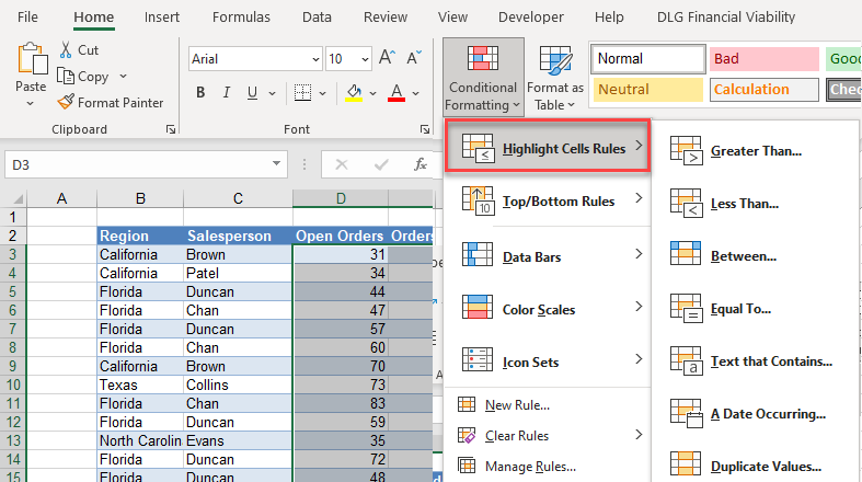
- Select the cells where you want to highlight certain values.
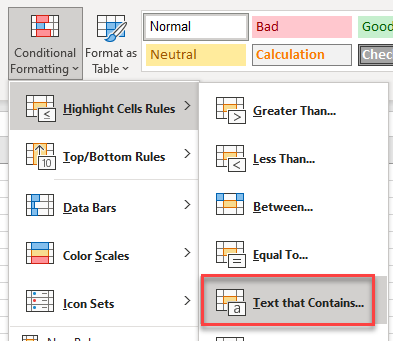
- Then, in the Ribbon, select Home > Conditional Formatting > Highlight Cells Rules.
The Highlight Cells Rules category allows you to select from greater than, less than, or equal to a certain value; between two set values; containing a text string; relating to a certain date; or containing a duplicated value.
- For this example, select Greater Than… and then type in the target number, where you want cells greater than that target highlighted, and select a format.
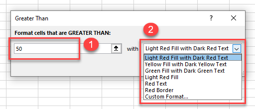
Note: Instead of typing in the actual value in the Format cells that are GREATER THAN box, you can click on a cell in your worksheet where you have a value stored. This would mean that if the value in that cell on your worksheet changed, the conditional formatting would change.
- Click OK.
Highlight Cells With Text
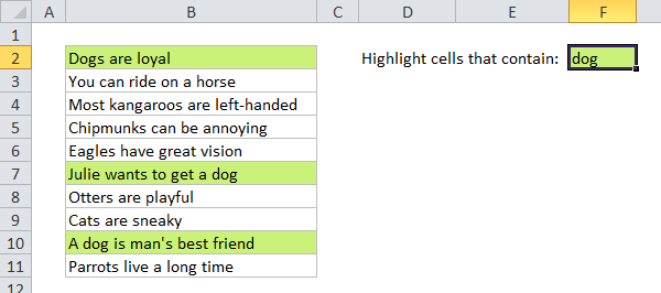
You can also test whether a cell contains a certain word or string of text using Highlight Cells Rules.
- Once again, select the cells where you want to highlight based on text.
- Then, in the Ribbon, select Home > Conditional Formatting > Highlight Cells Rules > Text that Contains…
- Type in your target text and select a format.
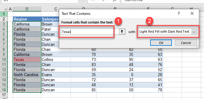
- Click OK.
Note: you can also type in part of a word or part of the text that is in the cell, you do not have to match the text entirely so typing as, for example, finds the cell with Texas in it.
Custom Rule
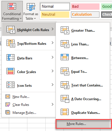
- In addition to these built-in Highlight Cells Rules, you can also create a custom rule by clicking on the More Rules… option at the bottom of the Highlight Cells Rules menu.
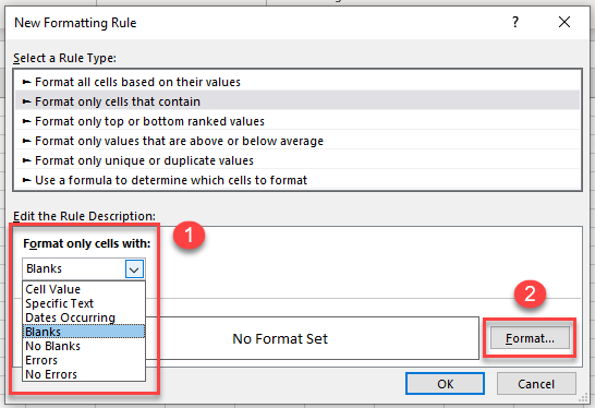
- Format only cells that contain is already highlighted. For this example, in the Format only cells with drop-down box, select Blanks.
- Then click Format…
- In the Format Cells window, choose a fill color, and press OK.
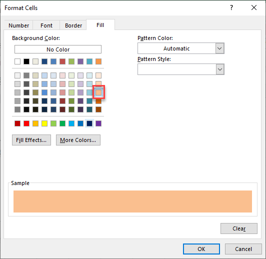
- Click OK once again to apply the conditional formatting to your cells.
Top/Bottom Rules
Top and bottom rules allow you to format cells according to the top or bottom values in a range. These rules only work on cells that contain values (not text!).
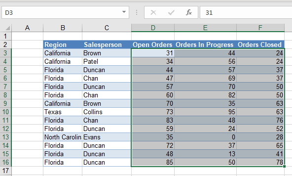
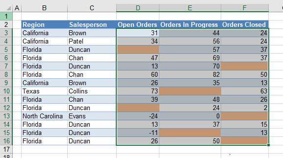
- Select the range where you want to highlight the highest or lowest values.
- Then, in the Ribbon, select Home > Conditional Formatting > Top/Bottom Rules.
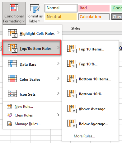
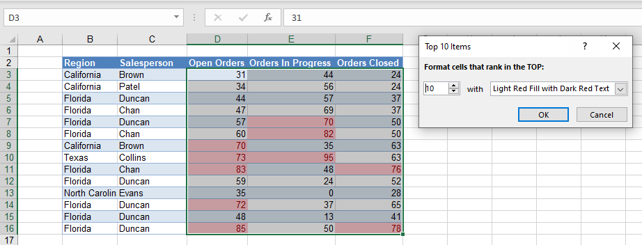
The Top/Bottom Rules category allows you to select from Top 10 Items, Top 10%, Bottom 10 Items, Bottom 10%, Above Average, or Below Average.
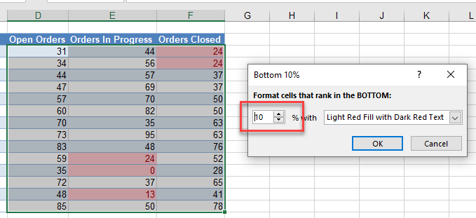
- For this example, select Bottom 10%…
- Adjust the target percentage up or down as needed, and then select a format. Click OK to apply the format to selected cells.
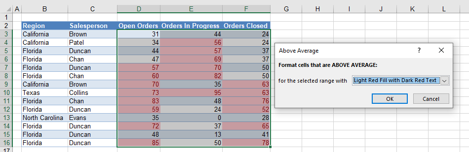
Note that you could also select Above Average or Below Average. These rules automatically calculate the mean of your data range and format cells either greater than or less than that value.
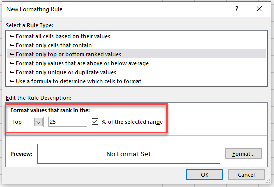
- To customize your rule even further, go back to the Top/Bottom Rules menu (from Step 2), and click More Rules… at the bottom.
- The rule type is selected for you (Format only top or bottom ranked values).
You can then edit the rule description by selecting either Top or Bottom in the drop-down list, and then typing in the comparison value (for example, 25, as shown below).
Check the % of the selected range if you want the top percentage of the values formatted rather than the actual top 25 values formatted.
- Set the format (see Steps 4 and 5 in the “Custom Rule” section), and then click OK to return to Excel.
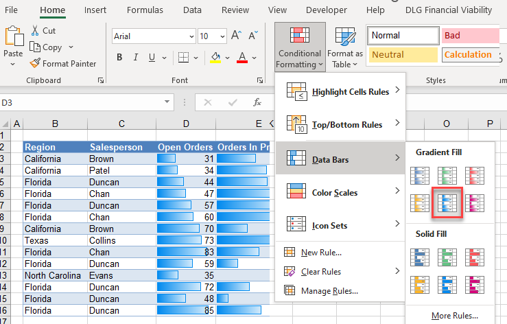
Data Bars
Data-bars rules add bars to each cell. The higher the value in the cell, the longer the bar is. These rules only work on cells that contain values (not text!).
- Select the cells where you want to show data bars.
- Then, in the Ribbon, select Home > Conditional Formatting > Data Bars.
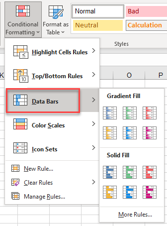
Data-bars rules allow you to select either a Gradient Fill or a Solid Fill bar in a variety of colors.
- To insert data bars into your cells, click on your preferred option.
- To customize your rule even further, click More Rules… at the bottom of the Data Bars menu.
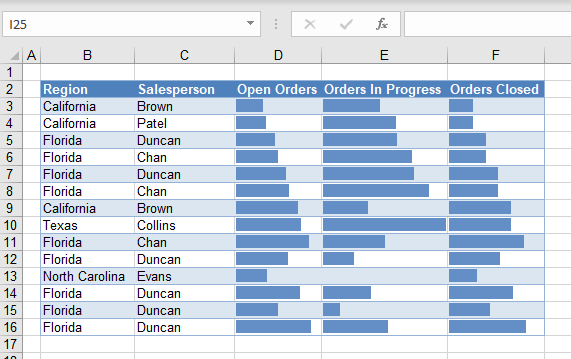
- The rule type is selected for you (Format all cells based on their values). For this example, check Show Bar Only, and then select the bar appearance (gradient or solid color). You can also choose to add border and choose the direction of the bars.
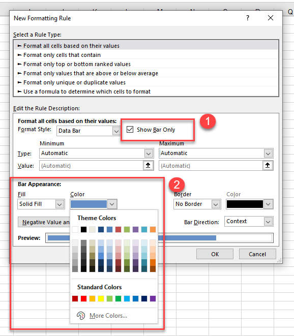
- Click OK to apply the formatting to selected cells.
Color Scales
Color-scales rules format cells according to their values relative to a selected range.
- Select the cells where you want to apply color scales.
- Then, in the Ribbon, select Home > Conditional Formatting > Color Scales.
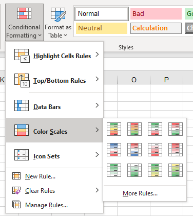
- To add a color scale to your cells, click on your preferred option.
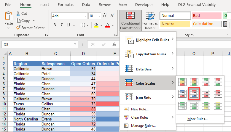
- To customize your rule even further, click More Rules… at the bottom of the Color Scales menu.
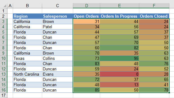
- The rule type is selected for you (Format all cells based on their values). Select a format style (either 2- or 3-color scale) and then set the values and colors you want.
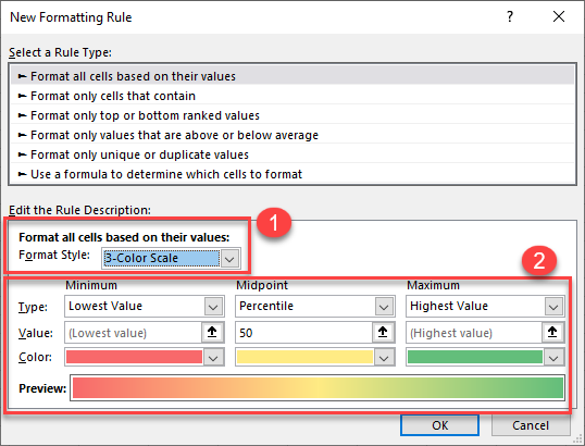
- Click OK to apply the formatting to your selected cells.
Icon Sets
There is one more built-in set of rules called Icon Sets. Click the link to learn about adding icon sets to your data.
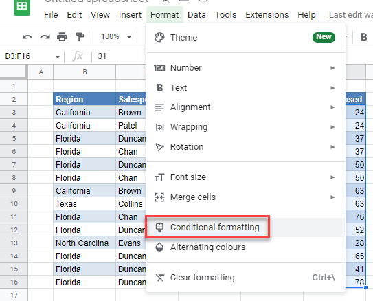
Format Based on Value or Text in Google Sheets
There are only two types of conditional formatting in Google Sheets: Single color and Color scale. Google Sheets’s Single color rules are similar to Highlight Cells Rules in Excel. Color scales rules are similar in the two applications as well.
Single Color
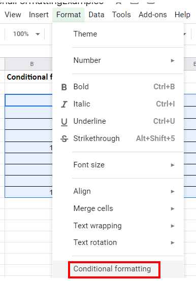
- Highlight the cells you wish to format, and then in the Menu, select Format > Conditional formatting.
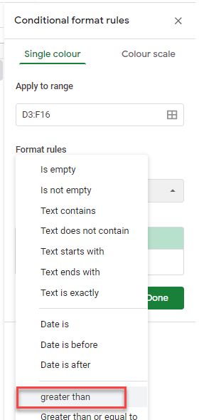
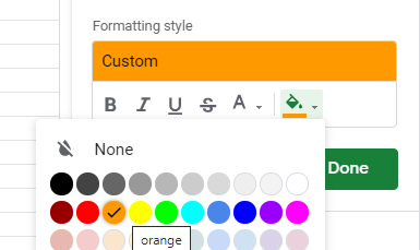
- In the format rules drop-down box, there is a long list of formats you can apply. For this example, select greater than.
- Type in the comparison value, and then click on the format drop down to select a fill color.
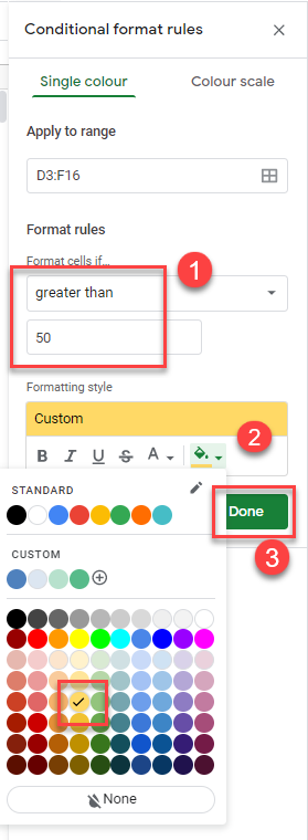
- Finally, click on Done to apply the formatting to selected cells.
Color Scale
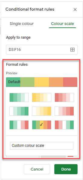
- To set a Color scale rule, click on Color scale in the Conditional formatting menu. In the format rules box, select an option to preview.
- You can then customize the Minpoint, Midpoint, and Maxpoint if you wish, or leave the default values.
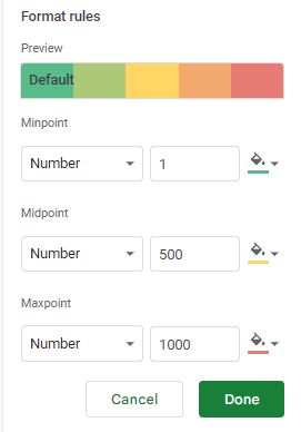
- Click Done to apply the formatting to your selected cells.
In this article we will learn how to color rows based on text criteria we use the “Conditional Formatting” option. This option is available in the “Home Tab” in the “Styles” group in Microsoft Excel.
Conditional Formatting in Excel is used to highlight the data on the basis of some criteria. It would be difficult to see various trends just for examining your Excel worksheet. Conditional Formatting in excel provides a way to visualize data and make worksheets easier to understand.
Excel Conditional Formatting allows you to apply formatting basis on the cell values such as colors, icons and data bars. For this, we will create a rule in excel Conditional Formatting based on cell value
How to write an if statement in excel?
IF function is used for logic_test and returns value on the basis of the result of the logic_test. Excel conditional formatting formula multiple conditions uses Statements like less than or equal to or greater than or equal to the value are used in IF formula
Syntax:
=IF (logical_test, [value_if_true], [value_if_false])
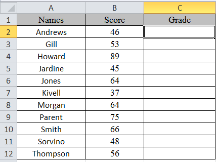
Let’s learn how to do conditional formatting in excel using IF function with the example.
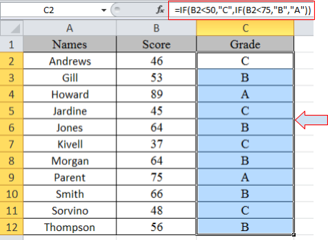
Here is a list of Names and their respective Scores.
multiple if statements excel functions are used here. So, there are 3 results based on the condition. if then statements in excel is used via excel conditional formatting formula
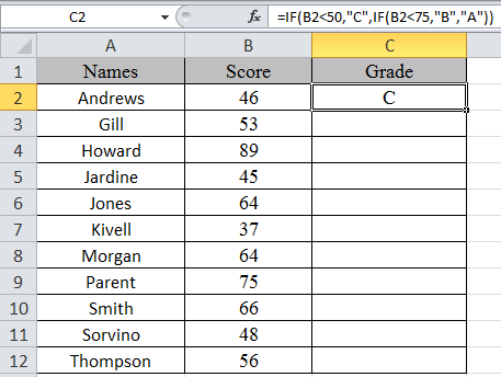
Write the formula in C2 cell.
Formula
=IF(B2<50,»C»,IF(B2<75,»B»,»A»))
Explanation:
IF function only returns 2 results, one [value_if_True] and Second [value-if_False]
First IF function checks, if the score is less than 50, would get C grade, The Second IF function tests if the score is less than 75 would get B grade and the rest A grade.
Copy the formula in other cells, select the cells taking the first cell where the formula is already applied, use shortcut key Ctrl + D
Now we will apply conditional formatting to it.
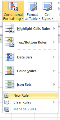
Select Home >Conditional Formatting > New Rule.
A dialog box appears
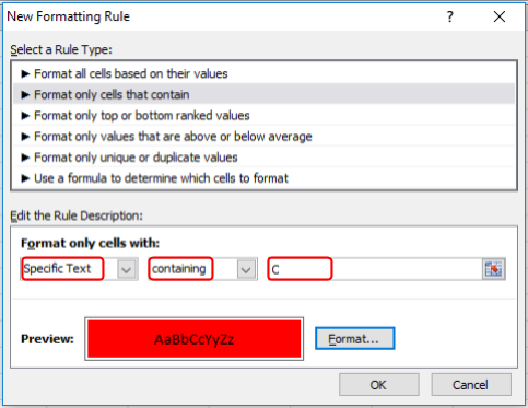
Select Format only cells that contain > Specific text in option list and write C as text to be formatted.
Fill Format with Red colour and click OK.
Now select the colour Yellow and Green for A and B respectively as done above for C.
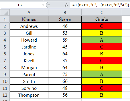
In this article, we used IF function and Conditional formatting tool to get highlighted grade.
As you can see excel change cell color based on value of another cell using IF function and Conditional formatting tool
Hope you learned how to use conditional formatting in Excel using IF function. Explore more conditional formulas in excel here. You can perform Conditional Formatting in Excel 2016, 2013 and 2010. If you have any unresolved query regarding this article, please do mention below. We will help you.
Related Articles:
How to use the Conditional formatting based on another cell value in Excel
How to use the Conditional Formatting using VBA in Microsoft Excel
How to use the Highlight cells that contain specific text in Excel
How to Sum Multiple Columns with Condition in Excel
Popular Articles:
50 Excel Shortcut to Increase Your Productivity
How to use the VLOOKUP Function in Excel
How to use the COUNTIF function in Excel 2016
How to use the SUMIF Function in Excel
Содержание
- Conditional Formatting If Between Two Numbers – Excel & Google Sheets
- Conditional Formatting if Between Two Numbers
- Alternate Method – Custom Formula
- Highlight Cells Between Two Numbers in Google Sheets
- Custom Formula in Google Sheets
- IF function
- Simple IF examples
- Common problems
- Need more help?
- Conditional formatting with formulas
- Summary
- Quick Links
- Quick start
- Formula logic
- Formula Examples
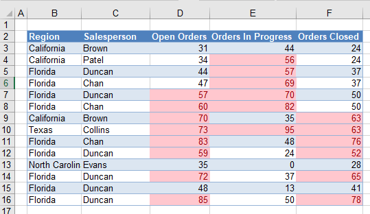
- Highlight orders from Texas
- Highlight dates in the next 30 days
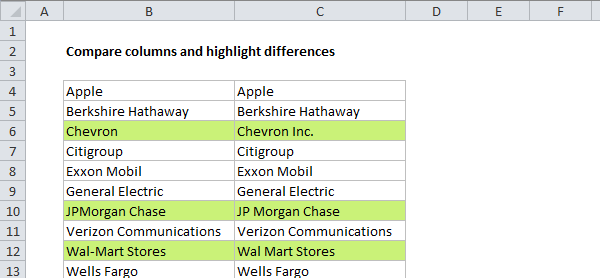
- Highlight column differences
- Highlight missing values
- Highlight properties with 3+ bedrooms under $350k
- Highlight top values (dynamic example)
- Gantt charts
- Simple search box
- Troubleshooting
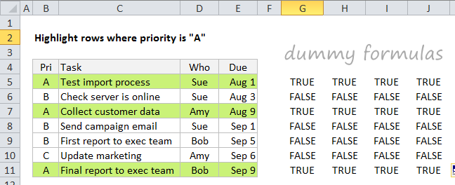
- Dummy Formulas
- Limitations
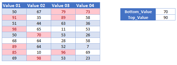
Conditional Formatting If Between Two Numbers – Excel & Google Sheets
This tutorial will demonstrate how to highlight cells that contain a value between two other specified values in Excel and Google Sheets.
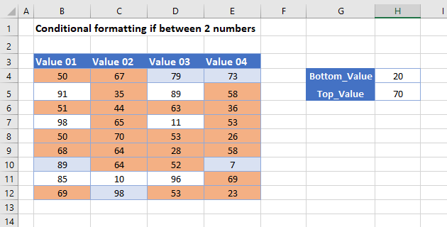
Conditional Formatting if Between Two Numbers
To highlight cells where the value is between a set minimum and maximum (inclusive), you can use one of the built-in Highlight Cell Rules within the Conditional Formatting menu.
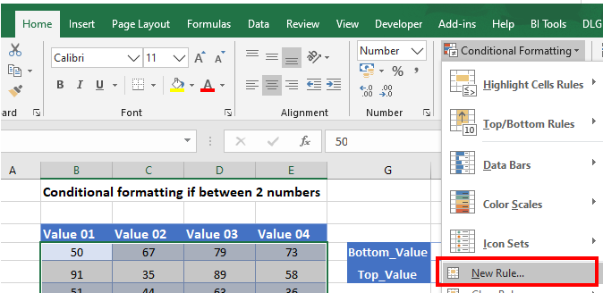
- Select the range you want to apply formatting to.
- In the Ribbon, select Home > Conditional Formatting > Highlight Cells Rules > Between…
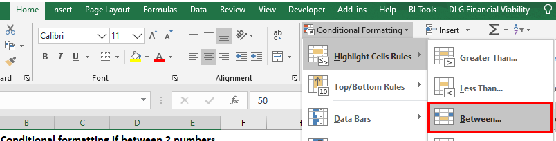
- You can either type in the bottom and top values, or to make the formatting dynamic (i.e., the result will change if you change the cells), click on the cells that contain the bottom and top values. Click OK.
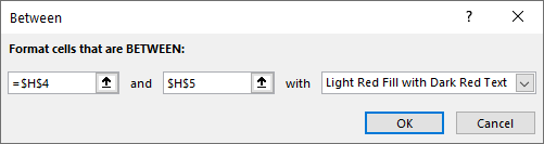
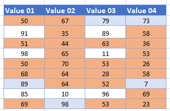
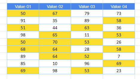
Values between 20 and 70 (inclusive) are highlighted.
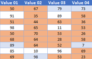
- When you change the two values in Cells H4 and H5, you obtain a different result.
Alternate Method – Custom Formula
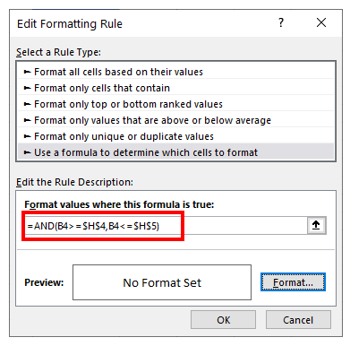
You can also highlight cells between two specified numbers by creating a New Rule and selecting Use a formula to determine which cells to format.
- Select New Rule from the Conditional Formatting menu.
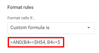
- Select Use a formula to determine which cells to format, and enter the formula (using the AND Function):
- The reference to cells H3 and H5 need to be locked by making them absolute. You can do this by using the $ sign around the row and column indicators, or by pressing F4 on the keyboard.
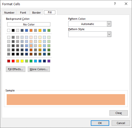
To learn more about how symbols are used in Excel, see How to Insert Signs and Symbols. - Click on the Format button.
- Choose a fill color for the highlighted cells.
- Click OK, then OK again to return to the Conditional Formatting Rules Manager.
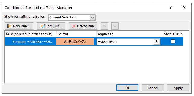
- Click Apply to apply the format to your worksheet.
Highlight Cells Between Two Numbers in Google Sheets
Highlighting cells between two numbers in Google Sheets is similar.
- Highlight the cells you wish to format, and then click on Format > Conditional Formatting.
- The Apply to Range section will already be filled in.

- From the Format Rules section, select Is Between from the drop-down list and set the minimum and maximum values.
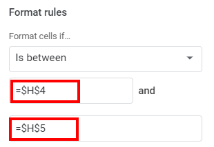
- Once again, you need to use the absolute signs (dollar signs) to lock in the values in Cells H4 and H5.
- Select the fill style for the cells that meet the criteria.
- Click Done to apply the rule.
Custom Formula in Google Sheets
- To use a custom formula rather than a built-in rule, select Custom formula is under Format Rules, and type the formula.
Remember to use $s or the F4 key to make Cells H4 and H5 absolute.
- Select your formatting and click Done.
Источник
IF function
The IF function is one of the most popular functions in Excel, and it allows you to make logical comparisons between a value and what you expect.
So an IF statement can have two results. The first result is if your comparison is True, the second if your comparison is False.
For example, =IF(C2=”Yes”,1,2) says IF(C2 = Yes, then return a 1, otherwise return a 2).

Use the IF function, one of the logical functions, to return one value if a condition is true and another value if it’s false.
IF(logical_test, value_if_true, [value_if_false])
The condition you want to test.
The value that you want returned if the result of logical_test is TRUE.
The value that you want returned if the result of logical_test is FALSE.
Simple IF examples

In the above example, cell D2 says: IF(C2 = Yes, then return a 1, otherwise return a 2)

In this example, the formula in cell D2 says: IF(C2 = 1, then return Yes, otherwise return No)As you see, the IF function can be used to evaluate both text and values. It can also be used to evaluate errors. You are not limited to only checking if one thing is equal to another and returning a single result, you can also use mathematical operators and perform additional calculations depending on your criteria. You can also nest multiple IF functions together in order to perform multiple comparisons.
 B2,”Over Budget”,”Within Budget”)» loading=»lazy»>
=IF(C2>B2,”Over Budget”,”Within Budget”)
In the above example, the IF function in D2 is saying IF(C2 Is Greater Than B2, then return “Over Budget”, otherwise return “Within Budget”)
 B2,C2-B2,»»)» loading=»lazy»>
In the above illustration, instead of returning a text result, we are going to return a mathematical calculation. So the formula in E2 is saying IF(Actual is Greater than Budgeted, then Subtract the Budgeted amount from the Actual amount, otherwise return nothing).

In this example, the formula in F7 is saying IF(E7 = “Yes”, then calculate the Total Amount in F5 * 8.25%, otherwise no Sales Tax is due so return 0)
Note: If you are going to use text in formulas, you need to wrap the text in quotes (e.g. “Text”). The only exception to that is using TRUE or FALSE, which Excel automatically understands.
Common problems
What went wrong
There was no argument for either value_if_true or value_if_False arguments. To see the right value returned, add argument text to the two arguments, or add TRUE or FALSE to the argument.
This usually means that the formula is misspelled.
Need more help?
You can always ask an expert in the Excel Tech Community or get support in the Answers community.
Источник
Conditional formatting with formulas

Summary
Although Excel ships with many conditional formatting «presets», these are limited. A more powerful way to apply conditional formatting is with formulas, because formulas allow you to apply rules that use more sophisticated logic. This article shows 10 examples, including how to highlight rows, column differences, missing values, and how to build Gantt charts and search boxes with conditional formatting.
Quick Links
Conditional formatting is a fantastic way to quickly visualize data in a spreadsheet. With conditional formatting, you can do things like highlight dates in the next 30 days, flag data entry problems, highlight rows that contain top customers, show duplicates, and more.
Excel ships with a large number of «presets» that make it easy to create new rules without formulas. However, you can also create rules with your own custom formulas. By using your own formula, you take over the condition that triggers a rule and can apply exactly the logic you need. Formulas give you maximum power and flexibility.
For example, using the «Equal to» preset, it’s easy to highlight cells equal to «apple».
But what if you want to highlight cells equal to «apple» or «kiwi» or «lime»? Sure, you can create a rule for each value, but that’s a lot of trouble. Instead, you can simply use one rule based on a formula with the OR function:
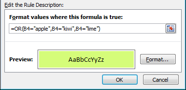
Here’s the result of the rule applied to the range B4:F8 in this spreadsheet:
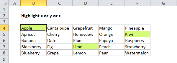
Here’s the exact formula used:
Quick start
You can create a formula-based conditional formatting rule in four easy steps:
1. Select the cells you want to format.
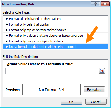
2. Create a conditional formatting rule, and select the Formula option
3. Enter a formula that returns TRUE or FALSE.
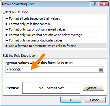
4. Set formatting options and save the rule.
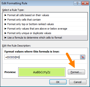
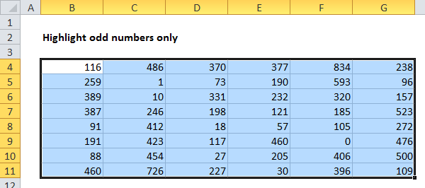
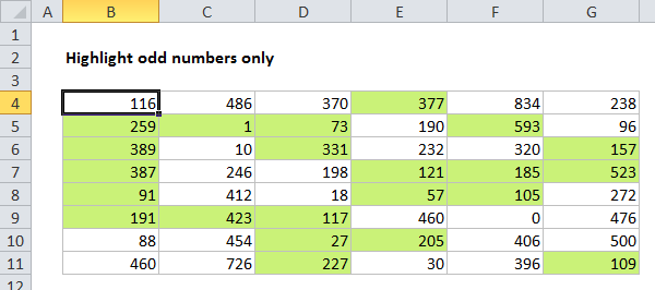
The ISODD function only returns TRUE for odd numbers, triggering the rule:
Formula logic
Formulas that apply conditional formatting must return TRUE or FALSE, or numeric equivalents. Here are some examples:
The above formulas all return TRUE or FALSE, so they work perfectly as a trigger for conditional formatting.
When conditional formatting is applied to a range of cells, enter cell references with respect to the first row and column in the selection (i.e. the upper-left cell). The trick to understanding how conditional formatting formulas work is to visualize the same formula being applied to each cell in the selection, with cell references updated as usual. Imagine that you entered the formula in the upper-left cell of the selection, and then copied the formula across the entire selection. If you struggle with this, see the section on Dummy Formulas below.
Formula Examples
Below are examples of custom formulas you can use to apply conditional formatting. Some of these examples can be created using Excel’s built-in presets for highlighting cells, but custom formulas can go far beyond presets, as you can see below.
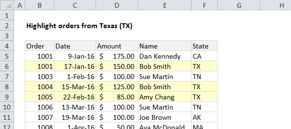
Highlight orders from Texas
To highlight rows that represent orders from Texas (abbreviated TX), use a formula that locks the reference to column F:
Highlight dates in the next 30 days
To highlight dates occurring in the next 30 days, we need a formula that (1) makes sure dates are in the future and (2) makes sure dates are 30 days or less from today. One way to do this is to use the AND function together with the NOW function like this:
With a current date of August 18, 2016, the conditional formatting highlights dates as follows:
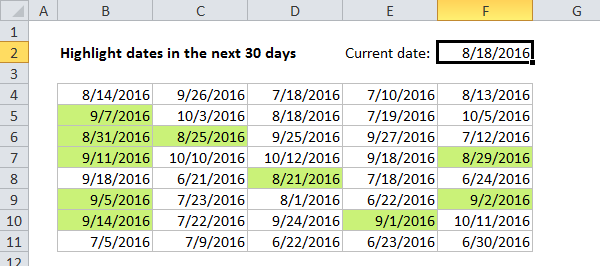
The NOW function returns the current date and time. For details about how this formula, works, see this article: Highlight dates in the next N days.
Highlight column differences
Given two columns that contain similar information, you can use conditional formatting to spot subtle differences. The formula used to trigger the formatting below is:
Highlight missing values
To highlight values in one list that are missing from another, you can use a formula based on the COUNTIF function:
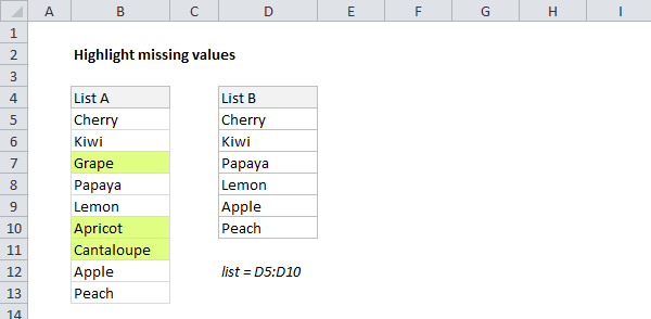
This formula simply checks each value in List A against values in the named range «list» (D5:D10). When the count is zero, the formula returns TRUE and triggers the rule, which highlights values in List A that are missing from List B.
Highlight properties with 3+ bedrooms under $350k
To find properties in this list that have at least 3 bedrooms but are less than $300,000, you can use a formula based on the AND function:
The dollar signs ($) lock the reference to columns C and D, and the AND function is used to make sure both conditions are TRUE. In rows where the AND function returns TRUE, the conditional formatting is applied:

Highlight top values (dynamic example)
Although Excel has presets for «top values», this example shows how to do the same thing with a formula, and how formulas can be more flexible. By using a formula, we can make the worksheet interactive — when the value in F2 is updated, the rule instantly responds and highlights new values.
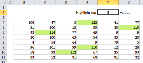
The formula used for this rule is:
Where «data» is the named range B4:G11, and «input» is the named range F2. This page has details and a full explanation.
Gantt charts
Believe it or not, you can even use formulas to create simple Gantt charts with conditional formatting like this:
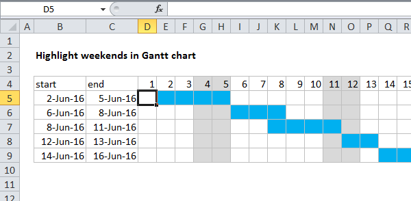
This worksheet uses two rules, one for the bars, and one for the weekend shading:
Simple search box
One cool trick you can do with conditional formatting is to build a simple search box. In this example, a rule highlights cells in column B that contain text typed in cell F2:
The formula used is:
For more details and a full explanation, see:
Troubleshooting
If you can’t get your conditional formatting rules to fire correctly, there’s most likely a problem with your formula. First, make sure you started the formula with an equals sign (=). If you forget this step, Excel will silently convert your entire formula to text, rendering it useless. To fix, just remove the double quotes Excel added at either side and make sure the formula begins with equals (=).
If your formula is entered correctly but is not triggering the rule, you may have to dig a little deeper. Normally, you can use the F9 key to check results in a formula or use the Evaluate feature to step through a formula. Unfortunately, you can’t use these tools with conditional formatting formulas, but you can use a technique called «dummy formulas».
Dummy Formulas
Dummy formulas are a way to test your conditional formatting formulas directly on the worksheet, so you can see what they’re actually doing. This can be a big time-saver when you’re struggling to get cell references working correctly.
In a nutshell, you enter the same formula across a range of cells that matches the shape of your data. This lets you see the values returned by each formula, and it’s a great way to visualize and understand how formula-based conditional formatting works. For a detailed explanation, see this article.
Limitations
There are some limitations that come with formula-based conditional formatting:
- You can’t apply icons, color scales, or data bars with a custom formula. You are limited to standard cell formatting, including number formats, font, fill color and border options.
- You can’t use certain formula constructs like unions, intersections, or array constants for conditional formatting criteria.
- You can’t reference other workbooks in a conditional formatting formula.
You can sometimes work around #2 and #3. You may be able to move the logic of the formula into a cell in the worksheet, then refer to that cell in the formula instead. If you are trying to use an array constant, try created a named range instead.
Источник
Conditional Formatting is one of the most simple yet powerful features in Excel Spreadsheets.
As the name suggests, you can use conditional formatting in Excel when you want to highlight cells that meet a specified condition.
It gives you the ability to quickly add a visual analysis layer over your data set. You can create heat maps, show increasing/decreasing icons, Harvey bubbles, and a lot more using conditional formatting in Excel.
Using Conditional Formatting in Excel (Examples)
In this tutorial, I’ll show you seven amazing examples of using conditional formatting in Excel:
- Quickly Identify Duplicates using Conditional Formatting in Excel.
- Highlight Cells with Value Greater/Less than a Number in a Dataset.
- Highlighting Top/Bottom 10 (or 10%) values in a Dataset.
- Highlighting Errors/Blanks using Conditional Formatting in Excel.
- Creating Heat Maps using Conditional Formatting in Excel.
- Highlight Every Nth Row/Column using Conditional Formatting.
- Search and Highlight using Conditional Formatting in Excel.
1. Quickly Identify Duplicates
Conditional formatting in Excel can be used to identify duplicates in a dataset.
Here is how you can do this:
This would instantly highlight all the cells that have a duplicate in the selected data set. Your dataset can be in a single column, multiple columns, or in a non-contiguous range of cells.

See Also: The Ultimate Guide to Find and Remove Duplicates in Excel.
2. Highlight Cells with Value Greater/Less than a Number
You can use conditional formatting in Excel to quickly highlight cells that contain values greater/less than a specified value. For example, highlighting all cells with sales value less than 100 million, or highlighting cells with marks less than the passing threshold.
Here are the steps to do this:
This would instantly highlight all the cells with values greater than 5 in a dataset. Note: If you wish to highlight values greater than equal to 5, you should apply conditional formatting again with the criteria “Equal To”.
The same process can be followed to highlight cells with a value less than a specified values.
3. Highlighting Top/Bottom 10 (or 10%)
Conditional formatting in Excel can quickly identify top 10 items or top 10% from a data set. This could be helpful in situations where you want to quickly see the top candidates by scores or top deal values in the sales data.
Similarly, you can also quickly identify the bottom 10 items or bottom 10% in a dataset.
Here are the steps to do this:
This would instantly highlight the top 10 items in the selected dataset. Note that this works only for cells that have a numeric value in it.
Also, if you have less than 10 cells in the dataset, and you select the options to highlight Top 10 items/Bottom 10 Items, then all the cells would get highlighted.
Here are some examples of how the conditional formatting would work:

4. Highlighting Errors/Blanks
If you work with a lot of numerical data and calculations in Excel, you’d know the importance of identifying and treating cells that have errors or are blank. If these cells are used in further calculations, it could lead to erroneous results.
Conditional Formatting in Excel can help you quickly identify and highlight cells that have errors or are blank.
Suppose we have a dataset as shown below:

This data set has a blank cell (A4) and errors (A5 and A6).
Here are steps to highlight the cells that are empty or have errors in it:
This would instantly highlight all the cells that are either blank or have errors in it.
 Note: You don’t need to use the entire range A1:A7 in the formula in conditional formatting. The above-mentioned formula only uses A1. When you apply this formula to the entire range, excel checks one cell at a time and adjusts the reference. For example, when it checks A1, it uses the formula =OR(ISBLANK(A1),ISERROR(A1)). When it checks cell A2, it then uses the formula =OR(ISBLANK(A2),ISERROR(A2)). It automatically adjusts the reference (as these are relative references) depending on which cell is being analyzed. So you need not write a separate formula for each cell. Excel is smart enough to change the cell reference all by itself 🙂
See Also: Using IFERROR and ISERROR to handle errors in excel.
5. Creating Heat Maps
A heat map is a visual representation of data where the color represents the value in a cell. For example, you can create a heat map where a cell with the highest value is colored green and there is a shift towards red color as the value decreases.
Something as shown below:

The above data set has values between 1 and 100. Cells are highlighted based on the value in it. 100 gets the green color, 1 gets the red color.
Here are the steps to create heat maps using conditional formatting in Excel.
- Select the data set.
- Go to Home –> Conditional Formatting –> Color Scales, and choose one of the color schemes.


As soon as you click on the heatmap icon, it would apply the formatting to the dataset. There are multiple color gradients that you can choose from. If you are not satisfied with the existing color options, you can select more rules and specify the color that you want.
Note: In a similar way, you can also apply Data Bard and Icon sets.
6. Highlight Every Other Row/Column
You may want to highlight alternate rows to increase the readability of the data.
These are called the zebra lines and could be especially helpful if you are printing the data.
Now there are two ways to create these zebra lines. The fastest way is to convert your tabular data into an Excel Table. It automatically applied a color to alternate rows. You can read more about it here.
Another way is using conditional formatting.
Suppose you have a dataset as shown below:

Here are the steps to highlight alternate rows using conditional formatting in Excel.
That’s it! The alternate rows in the data set will get highlighted.

You can use the same technique in many cases. All you need to do is use the relevant formula in the conditional formatting. Here are some examples:
- Highlight alternate even rows: =ISEVEN(ROW())
- Highlight alternate add rows: =ISODD(ROW())
- Highlight every 3rd row: =MOD(ROW(),3)=0
7. Search and Highlight Data using Conditional Formatting
This one is a bit advanced use of conditional formatting. It would make you look like an Excel rockstar.
Suppose you have a dataset as shown below, with Products Name, Sales Rep, and Geography. The idea is to type a string in cell C2, and if it matches with the data in any cell(s), then that should get highlighted. Something as shown below:

Here are the steps to create this Search and Highlight functionality:
That’s it! Now when you enter anything in cell C2 and hit enter, it will highlight all the matching cells.
How does this work?
The formula used in conditional formatting evaluates all the cells in the dataset. Let’s say you enter Japan in cell C2. Now Excel would evaluate the formula for each cell.
The formula would return TRUE for a cell when two conditions are met:
- Cell C2 is not empty.
- The content of cell C2 exactly matches the content of the cell in the dataset.
Hence, all the cells that contain the text Japan get highlighted.
Download the Example File

You can use the same logic, to create variations such as:
- Highlight the entire row instead of a cell.
- Highlight even when there is a partial match.
- Highlight the cells/rows as you type (dynamic) [You are going to love this trick :)].
How to Remove Conditional Formatting in Excel
Once applied, conditional formatting remains in place unless you remove it manually. As a best practice, keep the conditional formatting applied only to those cells where you need it.
Since it’s volatile, it may lead to a slow Excel workbook.
To remove conditional formatting:
- Select the cells from which you want to remove conditional formatting.
- Go to Home –> Conditional Formatting –> Clear Rules –> Clear Rules from Selected Cells.
- If you want to remove conditional formatting from the entire worksheet, select Clear Rules from Entire Sheet.

- If you want to remove conditional formatting from the entire worksheet, select Clear Rules from Entire Sheet.

Important things to know about Conditional Formatting in Excel
- Conditional formatting in volatile. It can lead to a slow workbook. Use it only when needed.
- When you copy paste cells that contain conditional formatting, conditional formatting also gets copied.
- If you apply multiple rules on the same set of cells, all rules remain active. In the case of any overlap, the rule applied last is given preference. You can, however, change the order by changing the order from the Manage Rules dialogue box.
You May Also Like the Following Excel Tutorials:
- The Right Way to Apply Conditional Formatting in Pivot Table
- Find and Remove Duplicates in Excel
- The Ultimate Guide to Using Conditional Formatting in Google Sheets
- How to Highlight Weekend Dates in Excel?
When you want to format a cell based on the value of a different cell, for example to format a report row based on a single column’s value, you can use the conditional formatting feature to create a formatting formula. This post explores the details of formatting a cell or range based on the value in another cell.
Objective
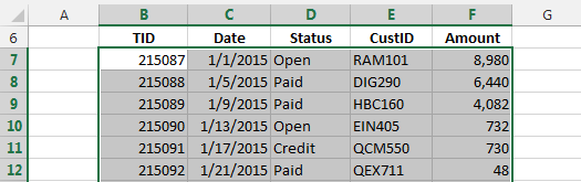
Here’s an example that will allow us to put this feature into context. Let’s say that you have an invoice listing and your objective is to identify the open invoices. Here is a screenshot of our sample invoice listing:
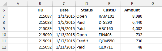
Since this is Excel, there are many ways to accomplish any given task. One way to identify the open invoices is to simply sort the list by the Status column so that the open invoices appear in a group. Another way is to filter the listing to show only the open invoices. These techniques are fairly straightforward, so, let’s explore another method. We’ll highlight the transaction rows with cell formatting…or, more precisely, a conditional formatting formula.
Video
Conditional Formatting Narrative
Using conditional formatting, it would be pretty easy to highlight just the Status column. It would be simple because the cells we are formatting are the same cells that have the values to evaluate. That is, we would be formatting a cell based on the value within that cell. To perform this, we could simply highlight the Status column, and the use the following Ribbon command:
- Home > Conditional Formatting > Cell Rules > Equal To
In the Equal To dialog box, we could enter the word “Open” and pick the desired formatting and click OK. Excel would then apply the formatting to the cells within the Status column that are equal to Open. While this technique is easy, it does not meet our goal which is to highlight the entire transaction row, not just the Status column.
To highlight the entire transaction row requires us to format a cell based on the value in another cell. That is, we want to format the TID, Date, Status, CustID, and Amount columns based on the value in the Status column. Considering a single cell for a moment, we want to format B7 based on the value in D7. This means that we want to format a cell, B7, based on the value in a different cell, D7. Expanding this to the entire row, we want to format B7:F7 based on the value in D7.
Excel makes it easy for users to format a cell based on the value of that cell, and the built-in conditional formatting rules use this logic. When we want to format a cell based on the value in a different cell, we’ll need to use a formula to define the conditional formatting rule. Fortunately, it is not very difficult to set up such a formatting formula.
Let’s highlight the entire transaction listing (B7:F36) first, and then open the conditional formatting dialog box using the following Ribbon icon:
- Home > Conditional Formatting > New Rule
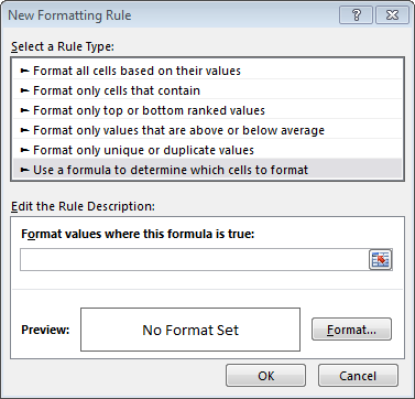
The New Formatting Rule dialog box has many choices, allowing you to, for example, format a cell based on the value, if it contains a value, the top or bottom ranked values, values that are above or below average, and unique or duplicate values. At the bottom of the list we find the option we need. We want to use a formula to determine which cells to format.
The formatting formula needs to be set up so that it returns a true or false value. If the formula returns true, then the desired formatting is applied. If the formula returns false, the formatting is not applied.
The key thing to understand about writing the formula is that the active cell is the reference point for the formula. Since this concept is absolutely critical, I don’t want to just skip through it, I want to unpack it for a moment.
You want to write the formatting formula as if you are writing it into the active cell and use the appropriate cell references and reference styles, such as absolute, relative, and mixed. If you can visualize the idea that you are writing the formula into the active cell, and the formula will be filled through the selected range, then writing the formula becomes easier. The formula you write will not be used to compute the cell value, rather, it will be used only for formatting.
Let’s assume that when we selected the entire transaction range, B7:F36 that the active cell is B7. When you select a range, there is still a single active cell. Check out the screenshot below to see that the range is selected, yet, B7 remains the active cell:
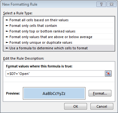
With this idea in mind, it is easy to write the conditional formatting formula now. We need to write the following formula in the New Formatting Rule dialog, as if we were writing it into cell B7:
=$D7="Open"
This simple comparison formula returns true when D7 is equal to Open, and thus, the desired format will be applied. Let’s take a quick look at the cell reference for a moment. We used a mixed cell reference, $D7, where the column part (D) is absolute and the row part (7) is relative. Here’s why. Remember we want to pretend that we are writing the formula into the active cell, in this case, B7. If we were only formatting B7, then, we could have used a relative reference D7, or an absolute reference $D$7, or a mixed reference. The reference style wouldn’t matter because the formula was used in a single cell only and was not filled anywhere.
However, the moment that we fill a formula down or to the right, we need to be careful to use the proper cell reference styles. In our case, as the formatting formula is filled right, we don’t want the column reference D to change. That is, for all cells, we want to reference the Status column, column D. To prevent Excel from changing the column reference as the formula is filed to the right, we lock it down with the dollar sign, resulting in $D. As the formatting formula is filled down throughout the selected range, we want to ensure that the row reference is updated accordingly. When formatting B7, we want to look at the Status column within the same row, or D7. However, when the formula is filled down to row 8, we want to format B8 based on the value in D8. Since we want Excel to update the row reference, we’ll leave it relative and not use the dollar sign to lock it down.
Here is a screenshot of the formatting dialog box with the formula:
Once the formula is entered, you simply use the Format button to specify the desired format.
Once the conditional formatting is applied to the range, the resulting worksheet is shown below:
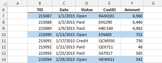
Bam…we got it!
FREE: Excel Speed Challenge
If you enjoyed this post, please check out our free Excel speed challenge.

Watch one short Excel video a day for 5 days. Total video time is only 45 minutes. Learn the Excel skills that can help you save an hour a week.
Other Considerations
In the formula above, we hard-coded the value, “Open” however, we could have easily placed this value into a cell, and then referenced the cell either by name or A1-style notation. In addition, besides just determining if the cell value is equal to a value, other comparison operators are supported, for example, greater than (>) and less than (<). We could have highlighted all rows where the value is greater than $5,000 by using the following comparison formula:
=$F7>5000
Since the formatting is applied based on a formula, we can get very creative and use worksheet functions. We could format alternating worksheet rows by using the MOD and ROW functions. Or, we could highlight old transactions by computing the difference between the transaction date and today’s date with the TODAY function. Indeed, this formatting formula provides many fun options.
Multiple Conditions
We can also use the logical AND and OR functions in case we want to consider multiple conditions. For example, formatting those rows where the status is open and the amount is greater than 5000 by using the following formula:
=AND($D7="Open",$F7>5000)
Since the AND function returns true when all of its arguments are true, the formatting is applied only when the status is open and the amount is greater than 5,000.
If we wanted to format the row if either condition was met, then we’d want to use the OR function instead of the AND function since it returns true if any single argument is true.
Conclusion
Having the ability to format a cell based on the value of another cell is quite handy. The key is to imagine that you are writing a formula into the active cell. The formula needs to use the appropriate cell reference styles (absolute, relative, mixed) so that as the formatting formula is filled throughout the selected range, the proper cells are considered. The sample file below has the conditional formatting rules included, so feel free to check it out.
Hope this helps, and remember, Excel rules!
Sample File
Here is the sample file in case you’d like to open it up and reference it.
FormattingFormula
The best part of conditional formatting is you can use formulas in it. And, it has a very simple sense to work with formulas.
Your formula should be a logical formula and the result should be TRUE or FALSE. If the formula returns TRUE, you’ll get the formatting, and if FALSE then nothing. The point is, by using formulas you can make the best out of conditional formatting.
Yes, that’s right. In the below example, we have used a formula in CF to check whether the value in the cell is smaller than 1000 or not.

And if that value is smaller than 1000 it will apply the formatting which we have specified, otherwise not. So today in this post, I’d like to share with you simple steps to apply conditional formatting using a formula. And some of the useful examples that you can use in your daily work.
Steps to Apply Conditional Formatting with Formulas
The steps to apply CF with formulas are quite simple:
- Select the range to apply Conditional Formatting.
- Add a formula to text a condition.
- Specify a format to apply when the condition is met.

To learn this in a proper way make sure to download this sample file from here and follow the below-detailed steps.
- First of all, select the range where you want to apply conditional formatting.

- After that, go to Home Tab ➜ Styles ➜ Conditional Formatting ➜ New Rule ➜ Use a formula to determine which cell to format.

- Now, in the “Format values where formula is true” enter the below formula.
=E5<1000

- The next thing is to specify the format to apply and for this, click on the format button and select the format.

- In the end, click OK.
While entering a formula in the CF dialog box you can’t see its result or whether that formula is valid or not. So, the best practice is to check that formula before using it in CF by entering it in a cell.
1. Use a Formula that is Based on Another Cell
Yes, you can apply conditional formatting based on another cell’s value. If you look at the below example, we have added a simple formula that is based on another cell. And if the value of that linked cell meets the condition specified, you’ll get conditional formatting.

When achievement will be below 75%, it will highlight in red color.

2. Conditional Formatting using IF
Whenever I think about conditions, the first thing that comes to my mind is using the IF function. And the best part of this function is, that it fits perfectly in conditional formatting. Let me show you an example:

Here, we have used the IF to create a condition and the condition is when the count of “Done” in range B3:B9 is equal to the count of tasks in the range A3:A9, then the final status will appear.
2. Conditional Formatting with Multiple Conditions
You can create multiple checks in conditions to apply to the format. Once all the conditions or one of the conditions will meet, conditional formatting will apply to the cell. Look at the below example where we have used the average temperature of my town.
And we have used a simply combined IF-AND to highlight the months when the temperature is pretty pleasant. Months where the temperature is between 15 Celsius to 35 Celsius, will get colored.
Just like this, you can also use if with or function.
4. Highlight Alternate Rows with Conditional Formatting
To highlight every alternate row you can use the following formula n CF.
=INT(MOD(ROW(),2))
By using this formula, every row whose number is odd will be highlighted. And, if you want to do vice versa you can use the following formula.

=INT(MOD(ROW()+1,2))
The same kind of formula can use for columns (odd and even) as well.
=INT(MOD(COLUMN(),2))
And for even columns.
=INT(MOD(COLUMN()+1,2))
5. Highlight Cells with Errors using CF
Now let’s come to another example where we will check whether a cell contains an error or not. What we need to do is just insert a formula in conditional formatting that can check the condition and return the result in TRUE or FALSE. You can even verify cells for numbers, text, or some specific values as well.

6. Create a Checklist with Conditional Formatting
Now let’s add some creativity to intelligence. You have already learned how to use a formula that is based on another cell. Here we have linked a checkbox with the B1 cell and further linked the B1 with the formula used in conditional formatting for cell A1.

Now, if you tick mark the checkbox, the value of cell B1 will turn into TRUE and cell A1 gets it conditional formatting [strikethrough].
Points to Remember
- Your formula should be a logical formula, which leads to a result as TRUE or FALSE.
- Try not to overload your data with conditional formatting.
- Always use relative and absolute references in a proper sense.
Sample File
Download this sample file from here to learn more.
More Tutorials
- AUTO FORMAT Option in Excel
- Apply Accounting Number Format in Excel
- Apply Background Color to a Cell or the Entire Sheet in Excel
- Print Excel Gridlines
- Add Page Number in Excel
- Apply Comma Style in Excel
- Apply Strikethrough in Excel
- Highlight Blank Cells in Excel
- Make Negative Numbers Red in Excel
- Cell Style (Title, Calculation, Total, Headings…) in Excel
- Change Date Format in Excel
- Highlight Alternate Rows in Excel with Color Shade
- Use Icon Sets in Excel (Conditional Formatting)
- Add Border in Excel
- Change Border Color in Excel
- Clear Formatting in Excel
- Copy Formatting in Excel
- Best Fonts for Microsoft Excel
- Hide Zero Values in Excel
⇠ Back to Advanced Excel Tutorials
Looking at a wad of numbers or a litany of texts, you cannot immediately interpret the relation between the values. Lowest prices, highest sales, changing trends, a specific text string, too much information.
Data can be filtered or sorted but how can you sort everything if you want one column showing descending values and the other showing ascending values? Here’s an idea, keep everything where it is and just spotlight the items of interest with some highlighting.
Our quickest understanding of data is very graphic and the best overview will also come through a play of colors and graphics. We’re starting to sound more and more like we’re hinting at Conditional Formatting and yes we are! Don’t know what Conditional Formatting is? Scroll ahead!
 1")
What is Conditional Formatting
Conditional Formatting is a feature in Excel that changes the display of cells whose values meet the Conditional Formatting rule’s criterion. Conditional Formatting makes it very easy to make note of important data whether numerical or non-numerical.
This feature uses graphic means such as highlighting, icons, and data bars to visually cast attention on the required group of values. By doing that, Conditional Formatting makes reviewing and visual analysis of data a very quick task without rearranging the data.
How Does Conditional Formatting Work?
Conditional Formatting applies to cells on the worksheet. At its very basic, you need to select the cells and then apply one of the Conditional Formatting rules. You can choose from the preset options or create your own rule (we will tell you how to do both).
The basic concept is that if a cell meets the Conditional Formatting condition, it results in TRUE and will be reformatted. If it results in FALSE, it won’t be reformatted.
The ease of Conditional Formatting is not only due to the visual impact, but also the automatic selection of the target data. Let’s say e.g., you want the sales figures over $1,000 highlighted below:
 2")
If this was a manual task, you would select the cells and then use Fill Color to flag the cells. With Conditional Formatting, you do not have to worry about selecting the right cells.
If you select all the data cells from column C, Conditional Formatting will do the job of flagging the right cells according to the set rule. Therefore, select all the cells with the sales figures:
 3")
Now where is this Conditional Formatting feature we’ve been talking about? In the Home tab, you will find the Conditional Formatting icon in the Styles group.
 4")
Conditional Formatting has highlighted the cells from the dataset that had sales of over $1,000:
 5")
Want to see how that’s done? Highlighting is not the only thing this feature does so you won’t get this formatting by just a click on the icon. Conditional Formatting has a bunch of options in its menu:
 6")
We’ll talk about creating different types of rules to conditionally format cells ahead in this tutorial.
Notes:
Conditional Formatting deals with numbers, dates, time, and text strings and while some rules won’t work for text, they all work for numbers, dates, and time (excluding the Text that Contains rule).
Conditional Formatting is dynamic. This means that it will adjust its result according to changes within the data. E.g. if a value that was previously not highlighted with Conditional Formatting is changed and meets the criterion of the applied rule, it will then be highlighted.
If you intend to make additional entries to the data and want Conditional Formatting to accommodate them, you can try leaving the references in the formula free if it doesn’t hinder the results of the Conditional Formatting rule(s).
E.g. enter B3 instead of $B$3. Another option is to force Conditional Formatting to include more rows/columns by using the Format Painter parallelly to the new row/column and then adding the data. Otherwise, you can simply extend the range in the Rules Manager.
Any Conditional Formatting action can be undone with Undo or Ctrl + Z including adding a new rule, deleting a rule, applying a rule, and editing a rule.
Cell Formatting You Can/Cannot Change
The format of a cell comprises several elements e.g., font size, font color, color fill, border, row height, etc. and there is only so much that Conditional Formatting can do. Some elements of the cell format can be changed by Conditional Formatting while others can’t. To keep your expectations real, let’s classify the elements of cell formats into what Conditional Formatting can and cannot change.
The Format Cells dialog box is what you will get when you click on the (Custom) Format button while dealing with a formatting rule. We can open Format Cells through Conditional Formatting and see what the feature will allow. Good idea. Let’s go through the Format Cells dialog box tab by tab, beginning with the Number tab:
 7")
All Number formats are applicable through Conditional Formatting including Custom Number Format.
The next tab is the Font tab:
 8")
In the Font tab, the elements of the font in the cell that we will be able to change with Conditional Formatting are font style (bold, italic, etc.), color, underline, and effects (strikethrough, superscript, etc.).
The rest of the elements that are grayed out are not accessible and cannot be changed using the Conditional Formatting feature. These are font family and size.
Moving on to the Border tab:
 9")
Border styles are changeable from the available options. The Border color can also be altered.
If you’re familiar with Borders in Excel, you’ll know that the Border styles in Conditional Formatting are limited. To be more specific, the double border and thicker borders are missing. So, the deduction is that border thickness cannot be changed with Conditional Formatting.
Let’s see what we can do fill-wise in the Fill tab:
 10")
All the Fill options can be edited in Conditional Formatting.
All in all, other than some font and border elements, all others can be changed through Conditional Formatting. Comparing this window to the regular Format Cells dialog box, we notice we have a couple of tabs missing; the Alignment and Protection tabs.
 11")
Conditional Formatting does not give access to these tabs which implies that the feature cannot change the text alignment or the protection of a cell via the feature.
Note:
Conditional Formatting is only a formatting feature and does not affect the value of a cell.
Conditional Formatting Options
Let’s refer back to the Conditional Formatting menu:
We’re going to tackle each item in this menu so…
Let’s get formatting! Conditionally though…
Highlight Cells Rules
One of the most commonly used features of Conditional Formatting is Highlight Cells. Selected cells will be highlighted according to a chosen cell highlighting rule. There are a few interesting preset rules available in this category e.g., highlighting a particular value, a cell that contains the given text, etc. Let’s go over all the options so you know how to apply them to your Excel work.
Greater Than…
The Greater Than rule highlights numerical values greater than the user-provided value. This option can be used to cast focus on high-performing products, the highest tier in an age group, amounts over a borderline value, etc. If that sounds like what you’re targeting, you can use the steps below to highlight cells with numerical values greater than the supplied value.
As an example, we’re taking some sales data categorized by product and state. For now, we want to find out which product is giving us the highest sales and from which region. Here’s how we do it:
- Select the relevant cells with the numeric values from where you want the highlighted cells.
 13")
- Select the Home tab’s Conditional Formatting icon in the Styles Point to Highlight Cells Rules and select the Greater Than rule.
 14")
- This rule will lead to a dialog box where you can set the numerical value and format intended for the highlighted cell. Gauging the selected cells, Excel will already provide you with an example value in the dialog box.
- In the Greater Than dialog box, adjust the numerical value in the text box. *(Read note below). The numbers that are greater than this number will be highlighted in the dataset. E.g. in our case, we want sales greater than $600 to be highlighted.
- You can also choose another format for the highlighted cells from the drop-down list in the dialog box.
 15")
- When done setting the number and format, click on the OK button of the dialog box.
The dialog box will close and the cells with sales greater than $600 will be highlighted in the chosen format:
 16")
Notes:
* The number $600 can also be added as a cell reference by clicking on the applicable cell with the blinking cursor in the text box of the dialog box. This would be the easier way if the value you want to set is a decimal.
By default, the highlight format for the cells will be light red fill with dark red text. This can quickly be changed to another ready format from the drop-down menu in the dialog box which also carries an option of a custom format. You’ll see how to set a custom highlight format in a while.
Less Than…
Let’s squeeze in the opposite of what we did just now in the same example. With the same concept, Conditional Formatting also gives the option of highlighting cells with values less than a provided number.
After applying this formatting rule in our case example, we’ll be able to see the top and flop products together on the same sheet, distinguished by a different format. See the steps and find out what that would look like:
- Select the data cells and go to the Conditional Formatting icon in the Home From the menu, head to Highlight Cells Rules and now select the Less Than option.
 17")
- Now you will have a Less Than dialog box, much like the one we saw earlier.
- Enter the number in the text field. Conditional Formatting will use this number to determine which cells should be highlighted. For our case, we are going with $150 so that values under 150 will be flagged.
- Change the format if you wish. We are aiming to highlight the bottom values so the default red format is good with us.
 18")
- Then hit the OK
From the selected cells, the products with sales lower than $150 are highlighted in the default red format:
 19")
Since we’ve used the Less Than rule with the Greater Than rule, we get a quick view of the hot and not products. Notice how we’re halfway to making a heat map?
Now that we mention it, Conditional Formatting is already ahead of us and allows us to create heat maps in Excel. How? You’ll see later. Hint: Color Scales.
Between…
The Between option highlights numerical values between 2 given numbers. This can be particularly helpful e.g., color coding an age group of interest. We’ll take a simple example and show you how it works.
In our simple example case, 10 people take part in a 5-question quiz to win a prize. A point is awarded for each question so we’d like to see how many participants scored averagely, say between 2 and 4. This is how to use Conditional Formatting to highlight values between 2 numbers inclusive:
- Select the number cells and open the Conditional Formatting menu from the Home Select Highlight Cells Rules > Between.
 20")
- A dialog box will appear for you to set the range of values and the highlighting format.
- Enter the numbers between which you want values highlighted in the dataset.
- This range works inclusively and the top and bottom values will also be highlighted.
- Choose a format for the highlighted cells and then click on the OK
 21")
We have set the values between 2 and 4 to be highlighted with a yellow fill:
 22")
Equal To…
But more importantly, wouldn’t you want to find out the winners? Of course you would. That would require highlighting the cells with a score of 5. Conditional Formatting makes highlighting cells carrying a specific value a task done in seconds.
Using the Equal To option in Highlight Cells Rules, we have mentioned the steps to highlight cells of a single value:
- Select the cells with the numbers.
- Go to Home tab > Conditional Formatting icon > Highlight Cells Rules > Equal To.
 23")
- In the text box in the Equal To dialog box, enter the number you want highlighted in the dataset and select the format for those highlighted cells.
 24")
- When you press the OK button, the entered number will be highlighted in the set format:
 25")
Text that Contains…
By now it looks like Highlight Cells Rules only likes working with numbers but that’s not the case. Have you ever had difficulty finding a part of text from a text string because it was not categorized appropriately?
We’ve been there too. If the target is to locate those cells or split the text, you can use Ctrl + F and other options to divide the text but if you want the text string found and the cell containing the text highlighted, nothing does it better than Conditional Formatting.
Follow the steps relating to the example ahead to find and highlight cells that contain the provided text with Conditional Formatting:
In this example, we have a list of fragrances with their brand names both mentioned together in column B. If we want to see which perfumes are made by a particular brand, taking e.g. Chanel, we will start by:
- Select the cells containing the data that you want to check.
- In the Conditional Formatting menu (Home tab > Style group), select Highlight Cells Rules and then the Text that Contains
 26")
- In the text field add the string of text you want to find in the data cells.
- To choose your format for the highlights, click on Custom Format from the drop-down menu.
 27")
- We’ve set a custom format with an orange color fill.
 28")
- Click OK on both windows to close them and apply Conditional Formatting to the cells in the custom format.
 29")
As per the set format and text value entered in the dialog box, the cells containing that text value will be highlighted:
 30")
A Date Occurring…
Another type of number value Conditional Formatting runs with is dates. With the A Date Occurring option, dates that range from the previous month to the next month can be highlighted.
For specific dates, you’ll have to resort to other Conditional Formatting rules since this rule does the job of highlighting dates relative to the current date e.g. dates from last week, yesterday, next month, etc.
Would be easier with an example? We think so too. Our example shows the order dates and scheduled delivery dates of a range of products. Take the current date as 25th of July. We want to highlight the dates from the list that are scheduled to be delivered the next day i.e. on the 26th of July.
With the following steps, you can use the A Date Occurring rule to highlight the date cells relative to the date option selected.
- Select the cells with the dates.
- Our target is to highlight the delivery date cells so we’ll select the date cells from column D.
 31")
- From the Home tab, select the Conditional Formatting button, Highlight Cells Rules, A Date Occurring.
 32")
- In the dialog box, open the first drop-down menu and select the required option.
- In our example, we want the dates for the next day highlighted and hence, we will go with the ‘Tomorrow’ option.
 33")
- Use the next drop-down menu to change the highlighted cells format.
 34")
The cells with the date 26th July 2022 in column D will be highlighted according to the selected format:
 35")
Note: The plus point of using A Date Occurring instead of forming a rule to highlight the 26th specifically is that this option will work relatively; with the changing date, the dates for the next day will automatically be highlighted e.g., on the 26th, 27th will be highlighted.
Duplicate Values…
When dealing with large data, there is a possibility of doubly-made entries and duplicate values. In most cases, you would want to avoid this and a good place to start would be to highlight them. Let’s see how to highlight repeat values with Conditional Formatting using an example.
In this example, we have used the RANDBETWEEN function to return 10 random numbers from 1 to 20. On its own, RANDBETWEEN doesn’t return unique numbers and there will be duplicates. Let’s check our data for duplicates with Conditional Formatting’s Duplicate Values option.
- Select the range you want to be searched for repetitions.
- From the Styles group in the Home tab, go to the Conditional Formatting’s Highlight Cells Rules menu and select Duplicate Values.
 36")
- In the dialog box, the default selection is “Duplicate” *(read note below) so you only need to change the default format if you want to.
 37")
- Select the OK command to close the dialog box and apply the Conditional Formatting for duplicate values:
 38")
* There is also an option to highlight unique values as shown in the example shot.
Top/Bottom Rules
We can now move on to the second item in the Conditional Formatting menu. The Top/Bottom Rules help the user format the top or bottom number values. In this set of rules, we have options for highlighting the top/bottom items, top/bottom x%, and the above/below average items.
Keep in mind that Top/Bottom Rules do not work on non-number values so text values, you’re out for now.
Also, we have a very interesting finding. The top/bottom percentage rule is a quick way to highlight the required percentile! If you’ve worked with percentiles before, you’ll find this particular feature rather handy.
Let’s start exploring the preset options in the Top/Bottom Rules one by one.
Top 10 Items…
Say you have a long list of expenses (don’t we all) and want to point out the top 10 items in the list that are taking up the most bucks. The top 5 priciest products, the top 15 songs from a database with the most hits; this is what you can use the Top 10 Items option for.
Another instance where you can use the Top 10 Items rule is the example ahead. We have the test marks out of 50 in a class of 10 students. Since our data consists of 10 students, we obviously won’t be searching for the top “10”.
Gladly, we can change this number. Let’s aim to find the top 3 scores on this test with Conditional Formatting’s Top 10 Items rule:
- Select the cells from the data containing the numbers, dates, or time.
 39")
- Now open the Conditional Formatting menu and go to Top/Bottom Rules and then Top 10 Items.
 40")
- The Top 10 Items dialog box has the number 10 suggested by default.
- Change the number ‘10’ according to your requirement using the spin button or by editing the value in the text box.
- At this point, you can also change the highlight format through the drop-down menu.
 41")
- To apply the format, close the dialog box with the OK
The top 3 items in the list are highlighted. In our case example, one of the marks has a repeat value i.e. 39 which is why you see 4 highlighted cells below:
 42")
The next rule in line is Top 10 % but we’ll bump up Bottom 10 Items because doesn’t that make a better succession to Top 10 Items?
Bottom 10 Items…
The Bottom 10 Items rule highlights, well yes, the bottom items. It works opposite of the Top 10 Items rule. Why would we want to bring the bottom items to notice? This could be for detecting the lowest performance products, months of lowest sales in a report, lowest scores, etc.
Taking the example from the section above, we will now study the 3 lowest scores. Looking at the range of bottom scores will help us ascertain if it’s just the lowest score that’s pulling the percentile down or if more students have scored similarly.
Let’s go ahead with using Conditional Formatting’s Bottom 10 Items rule to highlight the bottom 3 items in our case example:
- In the dataset, select the range with the numbers.
- From the Top/Bottom Rules in Conditional Formatting, select the Bottom 10 Items
 43")
- Change the number in the dialog box in line with the number of bottom items you want highlighted.
- Set the format of choice for the highlighted cells.
 44")
- When done, use the OK button to close the dialog box and highlight the relevant cells.
Here you can see that the bottom 3 items are highlighted in the chosen format:
 45")
The bottom 3 marks are 31, 33, and 34 showing that the lowest score is not the only reason for the lower percentiles since two other students out of 10 have scored likewise.
Top 10 %…
This is a very interesting rule. The Top 10 % rule works out the percentage from the numbers in the selected cells and highlights the cells with the numbers that fall in the top 10% (percentage can be adjusted).
With Excel putting in so much effort, isn’t life that much easier? Let’s find out if it is so! To highlight the top x% with Conditional Formatting use these steps:
- Begin with selecting the data cells with the numbers.
- Go to Home tab > Styles group > Conditional Formatting button > Top/Bottom Rules > Top 10 %.
 46")
- In the text field of the dialog box, you can change the percentage number which by default is set at 10.
- We’ll leave it at 10 since we are also aiming to calculate the top 10%. To calculate e.g. the bottom 25%, change this number to 25 in the dialog box.
- Use the drop-down menu in the dialog box to change the format of cells that are to be highlighted.
 47")
- Click on the OK button when done.
The marks falling in the top 10% of the selected cells will be highlighted:
 48")
Bottom 10 %…
After the Top 10 % follows the Bottom 10 %. The antithesis of what we just saw earlier, the Bottom 10 % rule takes the numbers in the selected cells to highlight the values that fall in the lower 10% of the numbers.
Carrying forward the previous example, let’s test how this rule works to highlight the bottom 10% with the top 10% already highlighted.
- Select the cells from the dataset and go to the Conditional Formatting options to select the Bottom 10 % rule in the Top/Bottom Rules.
 49")
- Set the format for highlighting and the number for the percentage in the Bottom 10% dialog box.
 50")
- When the OK command is pressed, the bottom 10% of the values will be highlighted.
 51")
Percentage or Percentile?
Let’s analyze what is happening here now that we’ve got the top and bottom 10% highlighted. And for discussion’s sake, we’re only talking about 10% here (though this can be any other percentage). If you think about regular percentage, 10% of 50 marks should be 5 marks so the top 10% (i.e. 90%) should be 45 marks.
In the Top 10 % rule, Conditional Formatting determines the top 10% only from the numbers selected. That means, this rule is unconcerned with the actual percentage because it is taking the lowest and highest values in the selection as 0% and 100%. Does that sound familiar? That is also the concept of percentile.
This finding is in line with percentile computations. If you look at the example shot above, we have calculated the 10th and 90th percentiles as 31.2 and 37.5 with the PERCENTILE.INC function. Compare this to the cells highlighted by Conditional Formatting.
For the top 10%, we have 31 marks highlighted (falls under 31.2 marks) and for the bottom 10%, 48 marks have been highlighted (going over 47.5 marks).
On this deduction, we can conclude that the Top and Bottom 10 % rules work as percentiles and can be a quick visual percentile map! Fascinating!
Above Average…
This section will further confirm the percentile theory. The Above Average rule in the Top/Bottom Rules highlights all the number values in the selection that are above the average of those numbers i.e. above 50% or the median.
Our previous example case has the median calculated using the PERCENTILE.INC function. Therefore, we’ll show you the steps to highlight the cells that are above the average of those numbers using Conditional Formatting’s Above Average rule.
- After selecting the cells with the numbers, click on the Conditional Formatting icon to access the Above Average option from the Top/Bottom Rules.
 52")
- You will be led to the Above Average dialog box:
- There is only one setting in this dialog box and i.e. the format of the highlighted cells.
- This rule only focuses on the average or 50% since the percentages can be adjusted in the Top and Bottom 10% rules.
 53")
- Hit OK when done and find one half of the values above average highlighted in the set format:
 54")
Below Average…
And for the other half of the average, this rule highlights the values from the cell selection that are below the average of those numbers.
Let’s piece this together with the case example from above and highlight the values below the average with Conditional Formatting’s Below Average rule with the steps mentioned ahead:
- Select the data with the numbers from where you want to calculate the average.
- Apply the Below Average rule by selecting Home tab, Conditional Formatting icon, Top/Bottom Rules, Below Average
 55")
- Set the preferred format for the highlighted values in the dialog box and click on the OK
 56")
The values below average in the selected cells will be highlighted in the set format:
 57")
Calculated as per the PERCENTILE.INC function, 50% of these numbers are above 37.5 marks, and 50% fall below. Evaluating the results of the highlights, we can see that Conditional Formatting tallies with the percentile system.
Data Bars
While numbers are crucial for calculations and analysis, the best type of data is one that is easily perceptible with distinguished high and low points. These two Conditional Formatting features (namely Data Bars and Color Scales) fulfill the convenience of giving the data a visual representation.
First comes Data Bars. Data Bars won’t be a very alien concept if you’ve seen bar charts. It’s like a personal bar for each cell.
Data Bars underlays a single bar in the selected cell. For a selected range, a bar will be added to each cell in line with and under the cell’s number value. The value of the cell determines and is directly proportional to the length of its Data Bar; small number – small bar.
In case you would ever want to add Data Bars to your dataset, we suggest these steps using Conditional Formatting in a simple example:
- Select the cells you want to add the Data Bars
- In the Home tab, head to the Styles group to access the Conditional Formatting Hover the cursor on Data Bars to reveal the menu. Choose the Data Bar style from the menu from Gradient Fill or Solid Fill. The color can also be chosen or you can create your own style from More Rules.
 58")
The Data Bars will be entered in the chosen style:
 59")
If you want to go for customized Data Bars, click on More Rules in the Data Bars menu.
 60")
In the Type fields, you have various options to change the type of Data Bar e.g., the one we just showed you was simply according to the numerical value. You can change this to percentile, percentage, etc. instead of numerical value.
These are fairly detailed options including changes for the bar direction (left to right, right to left) and Negative Value and Axis settings for when the data includes negative numbers.
Note: Data Bars and Icon Sets will also not affect the cell value as Conditional Formatting is only a formatting feature.
Color Scales
Remember we spoke of heat maps earlier? Now is a good time to come back to that. Excel can speedily ready a heat map for your dataset with Color Scales in Conditional Formatting. Think of it as color coding for the numbers in your data e.g., on a scale of red to green, the smallest number is red and the largest number is green. If you’re the one who had every color highlighter for studies or work, you’ll love this!
The perk of a Color Scale is that it can tell the position of any number in the range by the shade of the cell’s color. We’ll put Color Scales into action now with a very black and white example of product and state-wise categorized sales data.
 61")
- Select the relevant range for adding the Color Scale.
 62")
- Select Conditional Formatting from the Ribbon in the Home Hover the mouse pointer on Color Scales to open up some preset options.
Select the favored Color Scale or you can use the More Rules option to form a custom 2 or 3-Color Scale where you can also specify the minimum, mid (if any), and maximum values for the color points.
 63")
When the Color Scale is selected, it will be immediately applied to the selected range.
 64")
See how that works to give an instantaneous overview of the values? Maybe some of your highlighters have already made their way to the garbage.
Icon Sets
This is another very cool feature called Icon Sets that shows in what range a cell’s value lies according to its icon added by Conditional Formatting. Icon Sets applies a set of icons to the cells in selection. The Icon Sets represent the lowest, highest, and multiple mid (can be excluded) values that are editable.
Let’s apply Icon Sets in an example of quality assurance scores for 10 products. See what to do below to use Icon Sets in Conditional Formatting.
- Select the number cells for applying Icon Sets.
- Go to the Home tab > Conditional Formatting icon and point to the Icon Sets
- If you want to apply Icon Sets with the default settings* click on the relevant Icon Set from the menu. To change the settings according to which the icons will be added, click on the More Rules option in the Icon Sets menu.
 65")
- You will see a New Formatting Rule dialog box:
 66")
- Now make the changes as per your preference. These are the changes made for our case example:
- Pick the style from the Icon Style drop-down menu.
- Change the Type from Percentage to Number so that the Icons are entered according to the number of the cell, not the percentage of the number against all the selected cells.
- Set the numbers in the Value fields as the range for each icon. E.g. for values 12 and higher, a green check mark will be returned. Values between 8 and 11 will be assigned a yellow exclamation point and for lower numbers, there will be a red cross mark.
 67")
- If you want the numbers overwritten, click the Show Icon Only checkbox.
- Click on the OK button after the changes are made.
The Icon Set has been entered with the values in the selected cells in accordance with the changed settings:
 68")
* When applied, Icon Sets will enter icons to the selected cells in their default settings. The icons are set at equal percentage intervals e.g., a 3-Icon Set is applied at 33 percent intervals, 4-Icon Set at 25 percent intervals and 5-Icon Set at 20 percent intervals.
Tip: If you want the values and icons in separate columns, paste the values in another column, apply the Icon Set and overwrite the values by tick-marking the Show Icon Only checkbox in the settings.
Change Conditional Formatting Rule
To change a rule in Conditional Formatting, you need access to the Conditional Formatting Rules Manager. The Rule Manager enlists all the Conditional Formatting rules and allows changing, deleting, creating, and stacking rules according to preference of application.
You would want to change a rule in the case that an incorrect rule has been formed or some element of the rule needs editing and the original rule is not required anymore e.g., instead of the top 10 items, we want to highlight the top 3 items and don’t need to keep the top 10 items highlighted.
The original rule will not be overwritten if a new rule is formed.
See how to change a Conditional Formatting Rule using the steps written below:
- Select the range to which the rule applies.
- If you’re unclear about the range, you can select just a single cell or make a rough estimate of the range and the rules applied to the selected cell/range will be shown in the Rules Manager. Otherwise, you can select the entire sheet from the active worksheet or even from the Rules Manager.
- To open the Rules Manager, open the Conditional Formatting options from the Home tab and select Manage Rules.
 69")
- The Conditional Formatting Rules Manager lists the created rules for the cells selected on the worksheet. You can change this in the Show formatting rules for drop-down menu at the top in the Rules Manager.
 70")
- Select the rule you want to edit and click on the Edit Rule Alternatively, you can double-click a rule to edit it.
 71")
- Use the Edit Formatting Rule window to change the rule description and/or rule type.
 72")
- When you press the OK command, the edited rule will show in the Rules Manager.
 73")
- Press the OK button to apply the edited Conditional Formatting Rule.
 74")
As a result of the rule being changed from top 3 to top 2, only the top 2 numbers are highlighted in the example case above.
Delete Conditional Formatting Rule
Conditional Formatting Rules are deleted from the Conditional Formatting Rule Manager.
To completely remove a rule from the worksheet, you will have to delete the rule. It may also be easier to create a new rule instead of editing an old one in which case, you will have to delete the old rule. Deleting a rule is reversible by undoing the action so if you accidentally lose a rule, you can get it back.
Check these steps on how to delete a Conditional Formatting Rule:
- Select a cell in the range of the rule that you want to delete.
- Go to Home tab > Style group > Conditional Formatting > Manage Rules.
- This option opens the Conditional Formatting Rule Manager.
- Click on the rule and hit the Delete Rule
 76")
- The rule will be deleted without any confirmation. It’s not really a problem, if you delete the wrong rule, hit the Cancel command. If you’ve already pressed the OK button, you can hit Undo; the rule will be back.
- After deleting the rule, select the OK
The rule will be deleted and the formatting relevant to that rule will be cleared:
Deleting all Rules from Selection
One last thing left in the Conditional Formatting menu. While it’s easy to delete whichever rule from the Rules Manager, it can be tiresome carefully looking at absolutely referred ranges to see which rule applies where especially if you aim to delete the rules only from a specific range without deleting others.
To clear rules from a specific range, select the cells and go to Conditional Formatting icon > Clear Rules > Clear Rules from Selected Cells.
 78")
If you want to delete all the rules from the worksheet, you can go for Clear Rules from Entire Sheet instead of deleting the rules one by one from the Rules Manager. The other two options become available if there is an Excel Table or PivotTable present on the worksheet.
New Rule
New rules will not overwrite rules, they will be stacked (newest first unless the order is changed in the Rules Manager if any results are overlapping.
While more favorably you can create a new rule from Conditional Formatting’s New Rule option, a few options are also available in the Quick Analysis tool. The icon appears in the bottom-right corner when you select more than one data cell:
 79")
Click on this icon to see the options.
 80")
This is the little cousin of Conditional Formatting with 5 rules and an option to clear formatting from the selected area. Conditional Formatting in the Quick Analysis tool will add new rules to the selected range; it won’t overwrite rules.
New Formatting Rule Dialog Box
This dialog box will come into play with 3 actions; creating a new rule, editing a rule, and when you select More Rules in the Conditional Formatting menu. Most of the items in Rule Type are pretty much an extension of the options in the Conditional Formatting menu and some of them you will see in the sections later. Let’s quickly go over the Rule Types and what they contain.
Format all cells based on their values
This rule type has detailed options regarding Color Scales, Data Bars, and Icon Sets.
 81")
Format only cells that contain
This one’s intriguing. This rule type has varied options for formatting cells based on a specified value (number and text), date, blanks, no blanks, errors, and error-free cells.
 82")
Format only top or bottom ranked values
Here we can select top or bottom items or percentages to format the cells accordingly.
 83")
Format only values that are above or below average
This type is for widening the Above and Below Average rule in Conditional Formatting. We can format the cells with the average inclusive or exclusive and can also see some standard deviation options (hello math and stats).
 84")
Format only unique or duplicate values
Simply includes duplicate and unique values formatting.
 85")
Use a formula to determine which cells to format
If none of the preset rules and rule types suit your Excel action, you can get the needful done by entering a formula here.
 86")
Common Use Cases of Conditional Formatting
Now that we’ve covered everything contained in the Conditional Formatting menu, we can move on to scenarios that would commonly use Conditional Formatting. Some have already been discussed above. Let’s see what else Conditional Formatting can do.
Use Conditional Formatting to Highlight Alternate Rows
Highlighting alternate rows is nothing big for Conditional Formatting. And while this can also be done using a preset format in Excel Tables, you might not want to convert your range to a Table.
There are quite a few formulas that can be used with Conditional Formatting to highlight every other row. We’ll go with the one used in our example case below because it’s easy to tweak for your range and requirement. Let’s see the formula and how to apply it using Conditional Formatting to highlight alternate rows:
- On the worksheet, select the range where you want the alternately highlighted rows.
- Click on the Conditional formatting button in the Home tab and choose New Rule.
 87")
- There are 3 steps you need to take in the New Formatting Rule dialog box.
- In the Select a Rule Type section, choose Use a formula to determine which cells to format.
- In the given text box, enter this formula to highlight every other row:
=INT(MOD(ROW(),2))
Explanation below*
- Hit the Format button to set the format for the highlighted rows.
 88")
- One more step, select the OK
- That’s alternate rows highlighted for you with Conditional Formatting:
 89")
- The ROW function will take the number of the row the formula is entered in. Starting from the first row, in our example case, the number will be 3. The MOD function will return the remainder after 3 is divided by the supplied number 2. We are left with the number 1. The INT function is there to round the remainder down to an integer. Left with 1, the formula highlights the first row.
This formula can highlight even rows for you. So you can use this formula instead:
=INT(MOD(ROW()+1,2))
With the added 1, the formula will highlight the rows starting from the second row (the remainder 1 added to the extra 1 in this formula equals 2) in the range:
 90")
Use Conditional Formatting to Find & Highlight Blank Cell Rows
There are two aspects to highlighting blank cells in Excel. The first is only highlighting the blank cells. The second is highlighting the entire row or column in the dataset containing the blank cell.
Highlighting blank cells with Conditional Formatting doesn’t require any formula. There’s an in-built setting to highlight blank cells in the New Formatting Rule dialog box.
To enable it, select the area containing the blank cells and go to Conditional Formatting menu > New Rule. In the dialog box, select Format only cells that contain as the rule type and Blanks in the drop-down menu. Set the format.
 91")
This setting will highlight blank cells in the selected range. We had selected D6:D15.
 92")
To highlight the full row (let’s say from B7 to D7 when D7 is found blank), you’ll have to include a formula in the works so we can control highlighting the full row of the table. Here’s what you need to do to highlight the full row containing the blank cells with Conditional Formatting:
- Select the range in the dataset containing the blank cells. You need to select the area that you would want to be highlighted. In our case, the blank cells are among D6:D15 but we want the full row highlighted so we have to select the B6:D15.
- Create a new rule by selecting New Rule in the Conditional Formatting
 93")
- A New Formatting Rule dialog box will open. Make these changes in the dialog box:
- Click on the last option in Select a Rule Type field.
- Set the desired format for highlighting the rows.
- Enter this formula in the text box:
=COUNTBLANK($D6)
The reason we are using the COUNTBLANK function instead of ISBLANK is that our cells appear blank but contain a formula returning an empty text string. These will not be counted as blank by ISBLANK but COUNTBLANK will do the job for us.
Also note that the formula contains $D6 as the reference. This is the trick that highlights the full row in the selection. If the reference was D$6, the full column will be highlighted. For $D$6 as the reference, the mix of the two will be highlighted. Since we only want to highlight the full row of the selection, we’ve kept the row free with $D6.
 94")
- Hit the OK button when done.
Conditional Formatting will highlight, from the cell selection, the entire row with the empty cells:
 95")
Use Conditional Formatting to Highlight Overdue Dates
If you have a date-wise schedule for tasks and want to view the overdue tasks, Conditional Formatting makes that possible by highlighting the overdue date cells.
This can be done in 3 ways. Using the Less Than Highlighting Rule and entering the date. The dates before the given date will be returned.
But it won’t be possible to use the TODAY function in this method and neither will you be able to highlight the full row. The second method for conditionally formatting overdue dates involves the steps as follows:
- Select the date cells and create a new rule from the Conditional Formatting options from the Ribbon.
 96")
- Choose the second rule type in the dialog box.
- Select Cell Value and less than in the first and second fields of the Rule Description.
- Enter the formula mentioned ahead in the text box:
=TODAY()
- Set your preferred format for highlighted overdue dates.
 97")
- Press the OK command to create the new rule and highlight the overdue dates in the designated format:
 98")
The third way is to use the formula rule to add a complete formula that can be edited to highlight complete rows or columns instead of cells. No different from how we highlighted blank rows in the previous section.
Use Conditional Formatting to Compare Two Columns
When comparing columns for the the same or unique items, Conditional Formatting doesn’t leave much to work on our part as it can highlight duplicates or unique items in two (or more) lists. This will quickly give you an idea of common or even mismatched items especially if you are comparing columns linearly (line by line).
Earlier we showed you how to highlight duplicate numbers in a single column. Now let’s see how Conditional Formatting works to compare words in two columns. We’ll also switch it up to find unique values instead. Follow the steps below to compare two columns by highlighting unique values using Conditional Formatting:
- Select the data from the two columns that you want to compare.
- Select the Conditional Formatting icon > Highlight Cells Rules > Duplicate Values.
 99")
- Select Unique from the first drop-down menu in the Duplicate Values dialog box.
- Assign a format for the highlighted cells.
 100")
- Next, click on the OK
Return to the worksheet to find the unique values highlighted:
 101")
Use Conditional Formatting to Create Search and Format Box
This has to be the best of Excel tricks with Conditional Formatting and we’ve saved it for now! If whatever you enter in a particular cell will be searched on the sheet and highlighted, wouldn’t that be so cool to learn? We’re in the affirmative. There are a couple of ways to do this. One is to directly assign a formula to the data range. The steps to do this are right here:
- Assign a free cell on the worksheet as the search box.
- You can also label it. Highlight it in the same color that the searched and highlighted cells from the data would be. *(refer below)
 102")
- Select the range where the search will be targeted.
- For our case, we’ve selected B3 to B12.
- Make a new rule by selecting New Rule in the Conditional Formatting options in the Home
- In the dialog box, select Use a formula to determine which cells to format as the Rule Type.
- In the provided field, enter this formula:
=SEARCH($F$2,B3)
- This formula uses F2 as the search box and the target to be searched has been entered as B3 which will apply to the whole data range in column B. If you want to enter more columns as your search target, you can add the references using the & operator. E.g. if we were to include column C, we would refer B3&C3 or B3:C12 in the formula.
 103")
- Hit OK on the dialog box and you’re ready to go!
Now when you return to the worksheet, all your data range will be highlighted. Enter your search item in the search box and see the relevant cell(s) highlighted!
 104")
You can also try searching numbers:
 105")
The second method is to use a preset rule subject to highlight as per the search in F2. See how to do that with these steps:
- Select the data range for the search.
- Go to Conditional Formatting > Highlight Cells Rules > Text that Contains.
- In the given field, instead of entering any text, select the cell that you want to use as the search box.
 106")
You end up with the same search and format box!
*This will technically not have any impact on the search and format; it’s more like a reminder that the searched value will be highlighted this way (and let’s admit, when you see it working like that, it does look like Excel witchcraft).
Note: Search is not case-sensitive.
This is not where it ends. Likewise, you can enter the search box cell reference with other types of Conditional Formatting Rules too. And why stop at one? You can have multiple search boxes, each bound to a different rule e.g. two search boxes with upper and lower amounts where the upper one is used to highlight greater than quantities and the lower one for less than.
Use custom formats when you don’t want search boxes on the face of the sheet or when Conditional Formatting rules aren’t sufficient for your objective. Such custom formulas can be used for many tasks such as the ones we’ve seen in this tutorial. We’ll list a few examples with formulas that are to be used on the range containing the data:
Highlight Rows Meeting two Separate Conditions
To highlight e.g. those aged under 40 (column B) who took longer than 10 hours (column C) to complete a test:
=AND($B3<40,$C3>10)
 107")
Highlight Linear Differences
For highlighting linear differences between two lists:
=$B3<>$C3
 108")
Checked Box Strikes Text Through
For striking out tasks (with Strikethrough Font Effects) in a checklist when a checkbox is marked:
=IF(C3=TRUE,TRUE,FALSE)
The prerequisites for this Conditional Formatting rule are that you insert the checkboxes using Form Controls in the Developer tab and link each box to the cell it is in by right-clicking the checkbox, selecting Format Control, and linking the checkbox.
 109")
Highlight Cell when Target is Achieved
To highlight a cell when a total is met:
=IF(COUNTA($D$3:$D$20)>=18,TRUE,FALSE)
Enter this formula as a Conditional Formatting rule in the target cell F20. The trick is to enter the text “Daily target achieved!» in white font in F20 so that when the condition is met and the cell is highlighted in a dark color, the white text becomes visible.
 110")
Tip: If you find creating such formulas confusing or intimidating, you can apply the basic part of the formula in any free cell and apply Conditional Formatting in reference to that cell e.g. you apply the following formula in cell F19.
=COUNTA(D3:D25)
This will count the occupied cells for you (22 in this case). And then use this formula =$F$19>=18 in Conditional Formatting with F20 selected. Since 22 is greater than 18, F20 will be highlighted by Conditional Formatting which means that you will still achieve the same results.
We’re certain we’ve covered all the major and minor elements regarding Conditional Formatting in Excel as well as where and how it can be applied to achieve various results. Once you get around to using this feature, you’ll find it indispensable to quickly spot trends and anomalies and analyze data without changing its position.
Alright, we’re pretty sure you know that by now so about you try giving your worksheets a Conditional Formatting spin?
Combine conditional formatting with an IF statement
Syntax
=IF (logical_test, [value_if_true], [value_if_false])
But in conditional formatting, IF/THEN/ELSE syntax cannot be applied in a single rule. Conditional formatting is applied using IF/THEN logical test only. It must return TRUE for conditional formatting to be applied.
For example, if you want to apply conditional formatting using a condition that “If a cell value is greater than a set value, say 100, then format the cell as RED, else format the cell as GREEN”. So, you can see that it requires two rules to perform the conditional formatting, one for greater than 100, and one for less than 100.
You can apply more than one condition by creating more than one rule in conditional formatting. You can also use logical functions like AND and OR to create a rule set and apply conditional formatting in Excel.
Examples using conditional formatting with IF/THEN conditions
Let’s look at the scenarios to see how to use IF/THEN logical test in conditional formatting to highlight the targeted values. If you want to highlight the invoices in data range of A2:C13 which are due in the month of April, then you need to test the IF/THEN logical condition on date range in column B, if the month is equal to April, by using following custom formula in conditional formatting.=MONTH($B2)=4
First, select the data range A2:C13, then go to:
Conditional Formatting (on the Home tab) > New Rule> Use a formula to determine…> Enter the above formula in Edit Rule Description window> Choose the Format Fill to preview and press OK
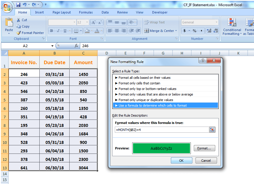
Please note that you have to fix the column by making it absolute using $ sign with it, and keep the row number free or relative to change. Hence, the formula will check each row of the specified column in the selected range, test the IF/THEN logical condition and will return TRUE and FALSE.
This rule will be evaluated in all active cells of locked column B one by one ignoring other cells in columns A and C. When the MONTH function in a cell of column B returns number 4 (April), the rule will return TRUE for all the active cells in that row and conditional formatting will be applied to that entire row as shown below.
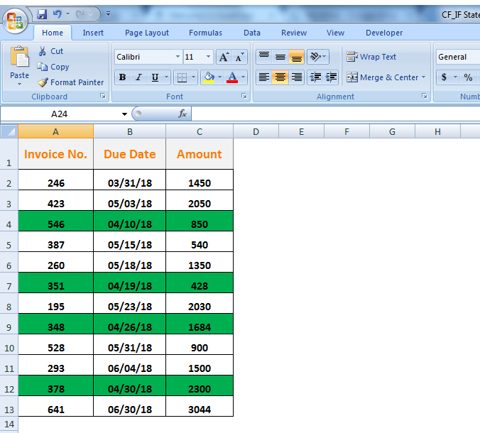
Now, if you want to conditionally highlight the two largest amount invoices due in the month of April, then you can achieve this by creating a rule set based on array formula using AND, LARGE and IF statement as per the following syntax.
=AND(criteria,$C2>=LARGE (IF(criteria, values),2)) =AND(MONTH($B2)=criteria,$C2>=LARGE (IF(MONTH(date)=criteria, amount),2)) =AND(MONTH($B2)=4,$C2>=LARGE(IF(MONTH($B$2:$B$13)=4,$C$2:$C$13),2))
By applying this custom formula, you can highlight the two largest amount invoices in the month of April. LARGE with IF function will generate a series of values and compare them with each value in column C. AND function will test the logical conditions in each cell of column B and C both one by one and will return TRUE where both conditions will be met. Have a look below.
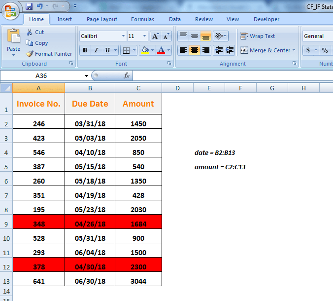
Need some additional help with Conditional Formatting or have other questions about Excel? Connect with a live Excel expert here for some 1 on 1 help. Your first session is always free.
Are you still looking for help with the Average function? View our comprehensive round-up of Average function tutorials here.