
IF function
The IF function is one of the most popular functions in Excel, and it allows you to make logical comparisons between a value and what you expect.
So an IF statement can have two results. The first result is if your comparison is True, the second if your comparison is False.
For example, =IF(C2=”Yes”,1,2) says IF(C2 = Yes, then return a 1, otherwise return a 2).

Use the IF function, one of the logical functions, to return one value if a condition is true and another value if it’s false.
IF(logical_test, value_if_true, [value_if_false])
For example:
-
=IF(A2>B2,»Over Budget»,»OK»)
-
=IF(A2=B2,B4-A4,»»)
|
Argument name |
Description |
|---|---|
|
logical_test (required) |
The condition you want to test. |
|
value_if_true (required) |
The value that you want returned if the result of logical_test is TRUE. |
|
value_if_false (optional) |
The value that you want returned if the result of logical_test is FALSE. |
Simple IF examples

-
=IF(C2=”Yes”,1,2)
In the above example, cell D2 says: IF(C2 = Yes, then return a 1, otherwise return a 2)

-
=IF(C2=1,”Yes”,”No”)
In this example, the formula in cell D2 says: IF(C2 = 1, then return Yes, otherwise return No)As you see, the IF function can be used to evaluate both text and values. It can also be used to evaluate errors. You are not limited to only checking if one thing is equal to another and returning a single result, you can also use mathematical operators and perform additional calculations depending on your criteria. You can also nest multiple IF functions together in order to perform multiple comparisons.

-
=IF(C2>B2,”Over Budget”,”Within Budget”)
In the above example, the IF function in D2 is saying IF(C2 Is Greater Than B2, then return “Over Budget”, otherwise return “Within Budget”)

-
=IF(C2>B2,C2-B2,0)
In the above illustration, instead of returning a text result, we are going to return a mathematical calculation. So the formula in E2 is saying IF(Actual is Greater than Budgeted, then Subtract the Budgeted amount from the Actual amount, otherwise return nothing).

-
=IF(E7=”Yes”,F5*0.0825,0)
In this example, the formula in F7 is saying IF(E7 = “Yes”, then calculate the Total Amount in F5 * 8.25%, otherwise no Sales Tax is due so return 0)
Note: If you are going to use text in formulas, you need to wrap the text in quotes (e.g. “Text”). The only exception to that is using TRUE or FALSE, which Excel automatically understands.
Common problems
|
Problem |
What went wrong |
|---|---|
|
0 (zero) in cell |
There was no argument for either value_if_true or value_if_False arguments. To see the right value returned, add argument text to the two arguments, or add TRUE or FALSE to the argument. |
|
#NAME? in cell |
This usually means that the formula is misspelled. |
Need more help?
You can always ask an expert in the Excel Tech Community or get support in the Answers community.

See Also
IF function — nested formulas and avoiding pitfalls
IFS function
Using IF with AND, OR and NOT functions
COUNTIF function
How to avoid broken formulas
Overview of formulas in Excel
Need more help?
Mikey556
New Member
- Joined
- Feb 9, 2022
- Messages
- 5
- Office Version
-
- 365
- Platform
-
- Windows
-
#1
Evening all!
In ‘Conditional Formats’ > ‘Use a formula to determine which cells to format’ I used the below condition to turn a cell green when my conditions were met, successfully:
=IF(TODAY()>=J14+J$7, TRUE())
I want the exact same condition, but for it to ADD 1 to a different cell.
How would I make that condition add +1 to cell A1 for example?
Thank you all for your time
Функция ЕСЛИ в Excel — это отличный инструмент для проверки условий на ИСТИНУ или ЛОЖЬ. Если значения ваших расчетов равны заданным параметрам функции как ИСТИНА, то она возвращает одно значение, если ЛОЖЬ, то другое.
Содержание
- Что возвращает функция
- Синтаксис
- Аргументы функции
- Дополнительная информация
- Функция Если в Excel примеры с несколькими условиями
- Пример 1. Проверяем простое числовое условие с помощью функции IF (ЕСЛИ)
- Пример 2. Использование вложенной функции IF (ЕСЛИ) для проверки условия выражения
- Пример 3. Вычисляем сумму комиссии с продаж с помощью функции IF (ЕСЛИ) в Excel
- Пример 4. Используем логические операторы (AND/OR) (И/ИЛИ) в функции IF (ЕСЛИ) в Excel
- Пример 5. Преобразуем ошибки в значения “0” с помощью функции IF (ЕСЛИ)
Что возвращает функция
Заданное вами значение при выполнении двух условий ИСТИНА или ЛОЖЬ.
Синтаксис
=IF(logical_test, [value_if_true], [value_if_false]) — английская версия
=ЕСЛИ(лог_выражение; [значение_если_истина]; [значение_если_ложь]) — русская версия
Аргументы функции
- logical_test (лог_выражение) — это условие, которое вы хотите протестировать. Этот аргумент функции должен быть логичным и определяемым как ЛОЖЬ или ИСТИНА. Аргументом может быть как статичное значение, так и результат функции, вычисления;
- [value_if_true] ([значение_если_истина]) — (не обязательно) — это то значение, которое возвращает функция. Оно будет отображено в случае, если значение которое вы тестируете соответствует условию ИСТИНА;
- [value_if_false] ([значение_если_ложь]) — (не обязательно) — это то значение, которое возвращает функция. Оно будет отображено в случае, если условие, которое вы тестируете соответствует условию ЛОЖЬ.
Дополнительная информация
- В функции ЕСЛИ может быть протестировано 64 условий за один раз;
- Если какой-либо из аргументов функции является массивом — оценивается каждый элемент массива;
- Если вы не укажете условие аргумента FALSE (ЛОЖЬ) value_if_false (значение_если_ложь) в функции, т.е. после аргумента value_if_true (значение_если_истина) есть только запятая (точка с запятой), функция вернет значение “0”, если результат вычисления функции будет равен FALSE (ЛОЖЬ).
На примере ниже, формула =IF(A1> 20,”Разрешить”) или =ЕСЛИ(A1>20;»Разрешить») , где value_if_false (значение_если_ложь) не указано, однако аргумент value_if_true (значение_если_истина) по-прежнему следует через запятую. Функция вернет “0” всякий раз, когда проверяемое условие не будет соответствовать условиям TRUE (ИСТИНА).
 |
| - Если вы не укажете условие аргумента TRUE(ИСТИНА) (value_if_true (значение_если_истина)) в функции, т.е. условие указано только для аргумента value_if_false (значение_если_ложь), то формула вернет значение “0”, если результат вычисления функции будет равен TRUE (ИСТИНА);
На примере ниже формула равна =IF (A1>20;«Отказать») или =ЕСЛИ(A1>20;»Отказать»), где аргумент value_if_true (значение_если_истина) не указан, формула будет возвращать “0” всякий раз, когда условие соответствует TRUE (ИСТИНА).

Функция Если в Excel примеры с несколькими условиями
Пример 1. Проверяем простое числовое условие с помощью функции IF (ЕСЛИ)
При использовании функции ЕСЛИ в Excel, вы можете использовать различные операторы для проверки состояния. Вот список операторов, которые вы можете использовать:
Ниже приведен простой пример использования функции при расчете оценок студентов. Если сумма баллов больше или равна «35», то формула возвращает “Сдал”, иначе возвращается “Не сдал”.
Пример 2. Использование вложенной функции IF (ЕСЛИ) для проверки условия выражения
Функция может принимать до 64 условий одновременно. Несмотря на то, что создавать длинные вложенные функции нецелесообразно, то в редких случаях вы можете создать формулу, которая множество условий последовательно.
В приведенном ниже примере мы проверяем два условия.
- Первое условие проверяет, сумму баллов не меньше ли она чем 35 баллов. Если это ИСТИНА, то функция вернет “Не сдал”;
- В случае, если первое условие — ЛОЖЬ, и сумма баллов больше 35, то функция проверяет второе условие. В случае если сумма баллов больше или равна 75. Если это правда, то функция возвращает значение “Отлично”, в других случаях функция возвращает “Сдал”.
Пример 3. Вычисляем сумму комиссии с продаж с помощью функции IF (ЕСЛИ) в Excel
Функция позволяет выполнять вычисления с числами. Хороший пример использования — расчет комиссии продаж для торгового представителя.
В приведенном ниже примере, торговый представитель по продажам:
- не получает комиссионных, если объем продаж меньше 50 тыс;
- получает комиссию в размере 2%, если продажи между 50-100 тыс
- получает 4% комиссионных, если объем продаж превышает 100 тыс.
Рассчитать размер комиссионных для торгового агента можно по следующей формуле:
=IF(B2<50,0,IF(B2<100,B2*2%,B2*4%)) — английская версия
=ЕСЛИ(B2<50;0;ЕСЛИ(B2<100;B2*2%;B2*4%)) — русская версия
В формуле, использованной в примере выше, вычисление суммы комиссионных выполняется в самой функции ЕСЛИ. Если объем продаж находится между 50-100K, то формула возвращает B2 * 2%, что составляет 2% комиссии в зависимости от объема продажи.
Больше лайфхаков в нашем Telegram Подписаться
Пример 4. Используем логические операторы (AND/OR) (И/ИЛИ) в функции IF (ЕСЛИ) в Excel
Вы можете использовать логические операторы (AND/OR) (И/ИЛИ) внутри функции для одновременного тестирования нескольких условий.
Например, предположим, что вы должны выбрать студентов для стипендий, основываясь на оценках и посещаемости. В приведенном ниже примере учащийся имеет право на участие только в том случае, если он набрал более 80 баллов и имеет посещаемость более 80%.
Вы можете использовать функцию AND (И) вместе с функцией IF (ЕСЛИ), чтобы сначала проверить, выполняются ли оба эти условия или нет. Если условия соблюдены, функция возвращает “Имеет право”, в противном случае она возвращает “Не имеет право”.
Формула для этого расчета:
=IF(AND(B2>80,C2>80%),”Да”,”Нет”) — английская версия
=ЕСЛИ(И(B2>80;C2>80%);»Да»;»Нет») — русская версия
Пример 5. Преобразуем ошибки в значения “0” с помощью функции IF (ЕСЛИ)
С помощью этой функции вы также можете убирать ячейки содержащие ошибки. Вы можете преобразовать значения ошибок в пробелы или нули или любое другое значение.
Формула для преобразования ошибок в ячейках следующая:
=IF(ISERROR(A1),0,A1) — английская версия
=ЕСЛИ(ЕОШИБКА(A1);0;A1) — русская версия
Формула возвращает “0”, в случае если в ячейке есть ошибка, иначе она возвращает значение ячейки.
ПРИМЕЧАНИЕ. Если вы используете Excel 2007 или версии после него, вы также можете использовать функцию IFERROR для этого.
Точно так же вы можете обрабатывать пустые ячейки. В случае пустых ячеек используйте функцию ISBLANK, на примере ниже:
=IF(ISBLANK(A1),0,A1) — английская версия
=ЕСЛИ(ЕПУСТО(A1);0;A1) — русская версия
The IF function runs a logical test and returns one value for a TRUE result, and another value for a FALSE result. The result from IF can be a value, a cell reference, or even another formula. By combining the IF function with other logical functions like AND and OR, you can test more than one condition at a time.
Syntax
The generic syntax for the IF function looks like this:
=IF(logical_test,[value_if_true],[value_if_false])The first argument, logical_test, is typically an expression that returns either TRUE or FALSE. The second argument, value_if_true, is the value to return when logical_test is TRUE. The last argument, value_if_false, is the value to return when logical_test is FALSE. Both value_if_true and value_if_false are optional, but you must provide one or the other. For example, if cell A1 contains 80, then:
=IF(A1>75,TRUE) // returns TRUE
=IF(A1>75,"OK") // returns "OK"
=IF(A1>85,"OK") // returns FALSE
=IF(A1>75,10,0) // returns 10
=IF(A1>85,10,0) // returns 0
=IF(A1>75,"Yes","No") // returns "Yes"
=IF(A1>85,"Yes","No") // returns "No"
Notice that text values like «OK», «Yes», «No», etc. must be enclosed in double quotes («»). However, numeric values should not be enclosed in quotes.
Logical tests
The IF function supports logical operators (>,<,<>,=) when creating logical tests. Most commonly, the logical_test in IF is a complete logical expression that will evaluate to TRUE or FALSE. The table below shows some common examples:
| Goal | Logical test |
|---|---|
| If A1 is greater than 75 | A1>75 |
| If A1 equals 100 | A1=100 |
| If A1 is less than or equal to 100 | A1<=100 |
| If A1 equals «Red» | A1=»red» |
| If A1 is not equal to «Red» | A1<>»red» |
| If A1 is less than B1 | A1<B1 |
| If A1 is empty | A1=»» |
| If A1 is not empty | A1<>»» |
| If A1 is less than current date | A1<TODAY() |
Notice text values must be enclosed in double quotes («»), but numbers do not. The IF function does not support wildcards, but you can combine IF with COUNTIF to get basic wildcard functionality. To test for substrings in a cell, you can use the IF function with the SEARCH function.
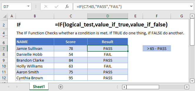
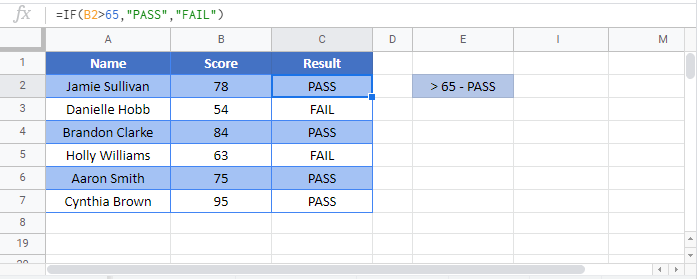
Pass or Fail example
In the worksheet shown above, we want to assign either «Pass» or «Fail» based on a test score. A passing score is 70 or higher. The formula in D6, copied down, is:
=IF(C5>=70,"Pass","Fail")
Translation: If the value in C5 is greater than or equal to 70, return «Pass». Otherwise, return «Fail».
Note that the logical flow of this formula can be reversed. This formula returns the same result:
=IF(C5<70,"Fail","Pass")
Translation: If the value in C5 is less than 70, return «Fail». Otherwise, return «Pass».
Both formulas above, when copied down, will return correct results.
Note: If you are new to the idea of formula criteria, this article explains many examples.
Assign points based on color
In the worksheet below, we want to assign points based on the color in column B. If the color is «red», the result should be 100. If the color is «blue», the result should be 125. This requires that we use a formula based on two IF functions, one nested inside the other. The formula in C5, copied down, is:
=IF(B5="red",100,IF(B5="blue",125))
Translation: IF the value in B5 is «red», return 100. Else, if the value in B5 is «blue», return 125.

There are three things to notice in this example:
- The formula will return FALSE if the value in B5 is anything except «red» or «blue»
- The text values «red» and «blue» must be enclosed in double quotes («»)
- The IF function is not case-sensitive and will match «red», «Red», «RED», or «rEd».
This is a simple example of a nested IFs formula. See below for a more complex example.
Return another formula
The IF function can return another formula as a result. For example, the formula below will return A1*5% when A1 is less than 100, and A1*7% when A1 is greater than or equal to 100:
=IF(A1<100,A1*5%,A1*7%)
Nested IF statements
The IF function can be «nested». A «nested IF» refers to a formula where at least one IF function is nested inside another in order to test for more conditions and return more possible results. Each IF statement needs to be carefully «nested» inside another so that the logic is correct. For example, the following formula can be used to assign a grade rather than a pass / fail result:
=IF(C6<70,"F",IF(C6<75,"D",IF(C6<85,"C",IF(C6<95,"B","A"))))
Up to 64 IF functions can be nested. However, in general, you should consider other functions, like VLOOKUP or XLOOKUP for more complex scenarios, because they can handle more conditions in a more streamlined fashion. For a more details see this article on nested IFs.
Note: the newer IFS function is designed to handle multiple conditions without nesting. However, a lookup function like VLOOKUP or XLOOKUP is usually a better approach unless the logic for each condition is custom.
IF with AND, OR, NOT
The IF function can be combined with the AND function and the OR function. For example, to return «OK» when A1 is between 7 and 10, you can use a formula like this:
=IF(AND(A1>7,A1<10),"OK","")
Translation: if A1 is greater than 7 and less than 10, return «OK». Otherwise, return nothing («»).
To return B1+10 when A1 is «red» or «blue» you can use the OR function like this:
=IF(OR(A1="red",A1="blue"),B1+10,B1)
Translation: if A1 is red or blue, return B1+10, otherwise return B1.
=IF(NOT(A1="red"),B1+10,B1)
Translation: if A1 is NOT red, return B1+10, otherwise return B1.
IF cell contains specific text
Because the IF function does not support wildcards, it is not obvious how to configure IF to check for a specific substring in a cell. A common approach is to combine the ISNUMBER function and the SEARCH function to create a logical test like this:
=ISNUMBER(SEARCH(substring,A1)) // returns TRUE or FALSEFor example, to check for the substring «xyz» in cell A1, you can use a formula like this:
=IF(ISNUMBER(SEARCH("xyz",A1)),"Yes","No")Read a detailed explanation here.
More information
- Read more about nested IFs
- Learn how to use VLOOKUP instead of nested IFs (video)
- 50 Examples of formula criteria
Notes
- The IF function is not case-sensitive.
- To count values conditionally, use the COUNTIF or the COUNTIFS functions.
- To sum values conditionally, use the SUMIF or the SUMIFS functions.
- If any of the arguments to IF are supplied as arrays, the IF function will evaluate every element of the array.
Содержание
- IF function
- Simple IF examples
- Common problems
- Need more help?
- Using IF with AND, OR and NOT functions
- Examples
- Using AND, OR and NOT with Conditional Formatting
- Need more help?
- See also
- Create conditional formulas
- What do you want to do?
- Create a conditional formula that results in a logical value (TRUE or FALSE)
- Example
- Create a conditional formula that results in another calculation or in values other than TRUE or FALSE
- Example
- IF function – nested formulas and avoiding pitfalls
- Remarks
- Examples
- Additional examples
- Did you know?
- Need more help?
IF function
The IF function is one of the most popular functions in Excel, and it allows you to make logical comparisons between a value and what you expect.
So an IF statement can have two results. The first result is if your comparison is True, the second if your comparison is False.
For example, =IF(C2=”Yes”,1,2) says IF(C2 = Yes, then return a 1, otherwise return a 2).
Use the IF function, one of the logical functions, to return one value if a condition is true and another value if it’s false.
IF(logical_test, value_if_true, [value_if_false])
The condition you want to test.
The value that you want returned if the result of logical_test is TRUE.
The value that you want returned if the result of logical_test is FALSE.
Simple IF examples
In the above example, cell D2 says: IF(C2 = Yes, then return a 1, otherwise return a 2)
In this example, the formula in cell D2 says: IF(C2 = 1, then return Yes, otherwise return No)As you see, the IF function can be used to evaluate both text and values. It can also be used to evaluate errors. You are not limited to only checking if one thing is equal to another and returning a single result, you can also use mathematical operators and perform additional calculations depending on your criteria. You can also nest multiple IF functions together in order to perform multiple comparisons.
B2,”Over Budget”,”Within Budget”)» loading=»lazy»>
=IF(C2>B2,”Over Budget”,”Within Budget”)
In the above example, the IF function in D2 is saying IF(C2 Is Greater Than B2, then return “Over Budget”, otherwise return “Within Budget”)
B2,C2-B2,»»)» loading=»lazy»>
In the above illustration, instead of returning a text result, we are going to return a mathematical calculation. So the formula in E2 is saying IF(Actual is Greater than Budgeted, then Subtract the Budgeted amount from the Actual amount, otherwise return nothing).
In this example, the formula in F7 is saying IF(E7 = “Yes”, then calculate the Total Amount in F5 * 8.25%, otherwise no Sales Tax is due so return 0)
Note: If you are going to use text in formulas, you need to wrap the text in quotes (e.g. “Text”). The only exception to that is using TRUE or FALSE, which Excel automatically understands.
Common problems
What went wrong
There was no argument for either value_if_true or value_if_False arguments. To see the right value returned, add argument text to the two arguments, or add TRUE or FALSE to the argument.
This usually means that the formula is misspelled.
Need more help?
You can always ask an expert in the Excel Tech Community or get support in the Answers community.
Источник
Using IF with AND, OR and NOT functions
The IF function allows you to make a logical comparison between a value and what you expect by testing for a condition and returning a result if that condition is True or False.
=IF(Something is True, then do something, otherwise do something else)
But what if you need to test multiple conditions, where let’s say all conditions need to be True or False ( AND), or only one condition needs to be True or False ( OR), or if you want to check if a condition does NOT meet your criteria? All 3 functions can be used on their own, but it’s much more common to see them paired with IF functions.
Use the IF function along with AND, OR and NOT to perform multiple evaluations if conditions are True or False.
IF(AND()) — IF(AND(logical1, [logical2], . ), value_if_true, [value_if_false]))
IF(OR()) — IF(OR(logical1, [logical2], . ), value_if_true, [value_if_false]))
IF(NOT()) — IF(NOT(logical1), value_if_true, [value_if_false]))
The condition you want to test.
The value that you want returned if the result of logical_test is TRUE.
The value that you want returned if the result of logical_test is FALSE.
Here are overviews of how to structure AND, OR and NOT functions individually. When you combine each one of them with an IF statement, they read like this:
AND – =IF(AND(Something is True, Something else is True), Value if True, Value if False)
OR – =IF(OR(Something is True, Something else is True), Value if True, Value if False)
NOT – =IF(NOT(Something is True), Value if True, Value if False)
Examples
Following are examples of some common nested IF(AND()), IF(OR()) and IF(NOT()) statements. The AND and OR functions can support up to 255 individual conditions, but it’s not good practice to use more than a few because complex, nested formulas can get very difficult to build, test and maintain. The NOT function only takes one condition.

Here are the formulas spelled out according to their logic:
=IF(AND(A2>0,B2 0,B4 50),TRUE,FALSE)
IF A6 (25) is NOT greater than 50, then return TRUE, otherwise return FALSE. In this case 25 is not greater than 50, so the formula returns TRUE.
IF A7 (“Blue”) is NOT equal to “Red”, then return TRUE, otherwise return FALSE.
Note that all of the examples have a closing parenthesis after their respective conditions are entered. The remaining True/False arguments are then left as part of the outer IF statement. You can also substitute Text or Numeric values for the TRUE/FALSE values to be returned in the examples.
Here are some examples of using AND, OR and NOT to evaluate dates.

Here are the formulas spelled out according to their logic:
IF A2 is greater than B2, return TRUE, otherwise return FALSE. 03/12/14 is greater than 01/01/14, so the formula returns TRUE.
=IF(AND(A3>B2,A3 B2,A4 B2),TRUE,FALSE)
IF A5 is not greater than B2, then return TRUE, otherwise return FALSE. In this case, A5 is greater than B2, so the formula returns FALSE.

Using AND, OR and NOT with Conditional Formatting
You can also use AND, OR and NOT to set Conditional Formatting criteria with the formula option. When you do this you can omit the IF function and use AND, OR and NOT on their own.
From the Home tab, click Conditional Formatting > New Rule. Next, select the “ Use a formula to determine which cells to format” option, enter your formula and apply the format of your choice.
 Edit Rule dialog showing the Formula method» loading=»lazy»>
Using the earlier Dates example, here is what the formulas would be.

If A2 is greater than B2, format the cell, otherwise do nothing.
=AND(A3>B2,A3 B2,A4 B2)
If A5 is NOT greater than B2, format the cell, otherwise do nothing. In this case A5 is greater than B2, so the result will return FALSE. If you were to change the formula to =NOT(B2>A5) it would return TRUE and the cell would be formatted.
Note: A common error is to enter your formula into Conditional Formatting without the equals sign (=). If you do this you’ll see that the Conditional Formatting dialog will add the equals sign and quotes to the formula — =»OR(A4>B2,A4
Need more help?
See also
You can always ask an expert in the Excel Tech Community or get support in the Answers community.
Источник
Create conditional formulas
Testing whether conditions are true or false and making logical comparisons between expressions are common to many tasks. You can use the AND, OR, NOT, and IF functions to create conditional formulas.
For example, the IF function uses the following arguments.
Formula that uses the IF function
 logical_test: The condition that you want to check.
 value_if_true: The value to return if the condition is True.
 value_if_false: The value to return if the condition is False.
For more information about how to create formulas, see Create or delete a formula.
What do you want to do?
Create a conditional formula that results in a logical value (TRUE or FALSE)
To do this task, use the AND, OR, and NOT functions and operators as shown in the following example.
Example
The example may be easier to understand if you copy it to a blank worksheet.
How do I copy an example?
Select the example in this article.
Selecting an example from Help
In Excel, create a blank workbook or worksheet.
In the worksheet, select cell A1, and press CTRL+V.
Important: For the example to work properly, you must paste it into cell A1 of the worksheet.
To switch between viewing the results and viewing the formulas that return the results, press CTRL+` (grave accent), or on the Formulas tab, in the Formula Auditing group, click the Show Formulas button.
After you copy the example to a blank worksheet, you can adapt it to suit your needs.
Determines if the value in cell A2 is greater than the value in A3 and also if the value in A2 is less than the value in A4. (FALSE)
Determines if the value in cell A2 is greater than the value in A3 or if the value in A2 is less than the value in A4. (TRUE)
Determines if the sum of the values in cells A2 and A3 is not equal to 24. (FALSE)
Determines if the value in cell A5 is not equal to «Sprockets.» (FALSE)
Determines if the value in cell A5 is not equal to «Sprockets» or if the value in A6 is equal to «Widgets.» (TRUE)
For more information about how to use these functions, see AND function, OR function, and NOT function.
Create a conditional formula that results in another calculation or in values other than TRUE or FALSE
To do this task, use the IF, AND, and OR functions and operators as shown in the following example.
Example
The example may be easier to understand if you copy it to a blank worksheet.
How do I copy an example?
Select the example in this article.
Important: Do not select the row or column headers.
Selecting an example from Help
In Excel, create a blank workbook or worksheet.
In the worksheet, select cell A1, and press CTRL+V.
Important: For the example to work properly, you must paste it into cell A1 of the worksheet.
To switch between viewing the results and viewing the formulas that return the results, press CTRL+` (grave accent), or on the Formulas tab, in the Formula Auditing group, click the Show Formulas button.
After you copy the example to a blank worksheet, you can adapt it to suit your needs.
=IF(A2=15, «OK», «Not OK»)
If the value in cell A2 equals 15, return «OK.» Otherwise, return «Not OK.» (OK)
=IF(A2<>15, «OK», «Not OK»)
If the value in cell A2 is not equal to 15, return «OK.» Otherwise, return «Not OK.» (Not OK)
=IF(NOT(A2 «SPROCKETS», «OK», «Not OK»)
If the value in cell A5 is not equal to «SPROCKETS», return «OK.» Otherwise, return «Not OK.» (Not OK)
If the value in cell A2 is greater than the value in A3 and the value in A2 is also less than the value in A4, return «OK.» Otherwise, return «Not OK.» (Not OK)
=IF(AND(A2<>A3, A2<>A4), «OK», «Not OK»)
If the value in cell A2 is not equal to A3 and the value in A2 is also not equal to the value in A4, return «OK.» Otherwise, return «Not OK.» (OK)
If the value in cell A2 is greater than the value in A3 or the value in A2 is less than the value in A4, return «OK.» Otherwise, return «Not OK.» (OK)
=IF(OR(A5<>«Sprockets», A6<>«Widgets»), «OK», «Not OK»)
If the value in cell A5 is not equal to «Sprockets» or the value in A6 is not equal to «Widgets», return «OK.» Otherwise, return «Not OK.» (Not OK)
=IF(OR(A2<>A3, A2<>A4), «OK», «Not OK»)
If the value in cell A2 is not equal to the value in A3 or the value in A2 is not equal to the value in A4, return «OK.» Otherwise, return «Not OK.» (OK)
For more information about how to use these functions, see IF function, AND function, and OR function.
Источник
IF function – nested formulas and avoiding pitfalls
The IF function allows you to make a logical comparison between a value and what you expect by testing for a condition and returning a result if True or False.
=IF(Something is True, then do something, otherwise do something else)
So an IF statement can have two results. The first result is if your comparison is True, the second if your comparison is False.
IF statements are incredibly robust, and form the basis of many spreadsheet models, but they are also the root cause of many spreadsheet issues. Ideally, an IF statement should apply to minimal conditions, such as Male/Female, Yes/No/Maybe, to name a few, but sometimes you might need to evaluate more complex scenarios that require nesting* more than 3 IF functions together.
* “Nesting” refers to the practice of joining multiple functions together in one formula.
Use the IF function, one of the logical functions, to return one value if a condition is true and another value if it’s false.
IF(logical_test, value_if_true, [value_if_false])
The condition you want to test.
The value that you want returned if the result of logical_test is TRUE.
The value that you want returned if the result of logical_test is FALSE.
While Excel will allow you to nest up to 64 different IF functions, it’s not at all advisable to do so. Why?
Multiple IF statements require a great deal of thought to build correctly and make sure that their logic can calculate correctly through each condition all the way to the end. If you don’t nest your formula 100% accurately, then it might work 75% of the time, but return unexpected results 25% of the time. Unfortunately, the odds of you catching the 25% are slim.
Multiple IF statements can become incredibly difficult to maintain, especially when you come back some time later and try to figure out what you, or worse someone else, was trying to do.
If you find yourself with an IF statement that just seems to keep growing with no end in sight, it’s time to put down the mouse and rethink your strategy.
Let’s look at how to properly create a complex nested IF statement using multiple IFs, and when to recognize that it’s time to use another tool in your Excel arsenal.
Examples
Following is an example of a relatively standard nested IF statement to convert student test scores to their letter grade equivalent.
 97,»A+»,IF(B2>93,»A»,IF(B2>89,»A-«,IF(B2>87,»B+»,IF(B2>83,»B»,IF(B2>79,»B-«,IF(B2>77,»C+»,IF(B2>73,»C»,IF(B2>69,»C-«,IF(B2>57,»D+»,IF(B2>53,»D»,IF(B2>49,»D-«,»F»))))))))))))» loading=»lazy»>
This complex nested IF statement follows a straightforward logic:
If the Test Score (in cell D2) is greater than 89, then the student gets an A
If the Test Score is greater than 79, then the student gets a B
If the Test Score is greater than 69, then the student gets a C
If the Test Score is greater than 59, then the student gets a D
Otherwise the student gets an F
This particular example is relatively safe because it’s not likely that the correlation between test scores and letter grades will change, so it won’t require much maintenance. But here’s a thought – what if you need to segment the grades between A+, A and A- (and so on)? Now your four condition IF statement needs to be rewritten to have 12 conditions! Here’s what your formula would look like now:
It’s still functionally accurate and will work as expected, but it takes a long time to write and longer to test to make sure it does what you want. Another glaring issue is that you’ve had to enter the scores and equivalent letter grades by hand. What are the odds that you’ll accidentally have a typo? Now imagine trying to do this 64 times with more complex conditions! Sure, it’s possible, but do you really want to subject yourself to this kind of effort and probable errors that will be really hard to spot?
Tip: Every function in Excel requires an opening and closing parenthesis (). Excel will try to help you figure out what goes where by coloring different parts of your formula when you’re editing it. For instance, if you were to edit the above formula, as you move the cursor past each of the ending parentheses “)”, its corresponding opening parenthesis will turn the same color. This can be especially useful in complex nested formulas when you’re trying to figure out if you have enough matching parentheses.
Additional examples
Following is a very common example of calculating Sales Commission based on levels of Revenue achievement.
 15000,20%,IF(C9>12500,17.5%,IF(C9>10000,15%,IF(C9>7500,12.5%,IF(C9>5000,10%,0)))))» loading=»lazy»>
This formula says IF(C9 is Greater Than 15,000 then return 20%, IF(C9 is Greater Than 12,500 then return 17.5%, and so on.
While it’s remarkably similar to the earlier Grades example, this formula is a great example of how difficult it can be to maintain large IF statements – what would you need to do if your organization decided to add new compensation levels and possibly even change the existing dollar or percentage values? You’d have a lot of work on your hands!
Tip: You can insert line breaks in the formula bar to make long formulas easier to read. Just press ALT+ENTER before the text you want to wrap to a new line.
Here is an example of the commission scenario with the logic out of order:
 5000,10%,IF(C9>7500,12.5%,IF(C9>10000,15%,IF(C9>12500,17.5%,IF(C9>15000,20%,0)))))» loading=»lazy»>
Can you see what’s wrong? Compare the order of the Revenue comparisons to the previous example. Which way is this one going? That’s right, it’s going from bottom up ($5,000 to $15,000), not the other way around. But why should that be such a big deal? It’s a big deal because the formula can’t pass the first evaluation for any value over $5,000. Let’s say you’ve got $12,500 in revenue – the IF statement will return 10% because it is greater than $5,000, and it will stop there. This can be incredibly problematic because in a lot of situations these types of errors go unnoticed until they’ve had a negative impact. So knowing that there are some serious pitfalls with complex nested IF statements, what can you do? In most cases, you can use the VLOOKUP function instead of building a complex formula with the IF function. Using VLOOKUP, you first need to create a reference table:

This formula says to look for the value in C2 in the range C5:C17. If the value is found, then return the corresponding value from the same row in column D.

Similarly, this formula looks for the value in cell B9 in the range B2:B22. If the value is found, then return the corresponding value from the same row in column C.
Note: Both of these VLOOKUPs use the TRUE argument at the end of the formulas, meaning we want them to look for an approxiate match. In other words, it will match the exact values in the lookup table, as well as any values that fall between them. In this case the lookup tables need to be sorted in Ascending order, from smallest to largest.
VLOOKUP is covered in much more detail here, but this is sure a lot simpler than a 12-level, complex nested IF statement! There are other less obvious benefits as well:
VLOOKUP reference tables are right out in the open and easy to see.
Table values can be easily updated and you never have to touch the formula if your conditions change.
If you don’t want people to see or interfere with your reference table, just put it on another worksheet.
Did you know?
There is now an IFS function that can replace multiple, nested IF statements with a single function. So instead of our initial grades example, which has 4 nested IF functions:
It can be made much simpler with a single IFS function:
The IFS function is great because you don’t need to worry about all of those IF statements and parentheses.
Note: This feature is only available if you have a Microsoft 365 subscription. If you are a Microsoft 365subscriber, make sure you have the latest version of Office.
Need more help?
You can always ask an expert in the Excel Tech Community or get support in the Answers community.
Источник
The syntax of the IF() function is the following:
= IF ( logical_test , [value_if_TRUE] , [value_if_FALSE] )
The first two attributes are obligatory, i.e. without them, the formula doesn’t work, and produces an error message.
- logical _test – a placeholder for the condition we want to test
- value_if_TRUE – an attribute where we need to specify a value (text, or another function) that the IF formula returns when the result of the logical_test is TRUE
The third parameter is Optional, i.e. we can skip it and in such a case, the IF() function returns the default value FALSE.
- value_if_FALSE – an attribute for a value, text or another formula that the IF() function must return when the result of the logical test is FALSE.
In other words, IF() function is used to test the specific conditions and can be described as the statement:
IF something is true, THEN return the first value, ELSE – return then second value.
The simplest IF() function may be written with the first two parameters only.
For example, this formula is absolutely correct:
=IF(C2=1,"Hello!")This formula tests the condition we set (C2=1) and if it is true, the formula returns the text message (“Hello!”).
Otherwise, it returns the default value FALSE.
Interesting Fact!!! You can use another simpler test in Excel for a certain condition. Just place a formula like “=C2>C3” in a cell and press ENTER. If this statement is true, the formula returns the default value – TRUE. Else (i.e. when a value in C2 is NOT larger than a value in C3 cell) the formula will return another default value – FALSE. We use the IF() function in these cases; when we want to trigger some further actions or calculations depending on the results of the logical test.
Typically, the IF() function is used in situations when we need to calculate or flag the results based on certain conditions (for example, smaller than, equal to, greater than and others).
Despite the fact that Excel usually provides multiple choices on how to solve every specific task, the IF() function can play a good role in such cases.
Another simple example of the IF() function:
=IF(C3="Hello!",1, 0)If a value of the C3 cell is the text “Hello!” then this formula returns the one (1) value.
Else (i.e. if this cell contains any other text, number or blank value), the formula returns zero.
The big advantage of the IF() function (like many other Excel functions) is how we can replace all three arguments in this example with whatever we want/need and it still works properly (if we follow the syntax, of course).
For example, let’s replace the one (as a value_if_true) to another formula “C3+C4” and replace zero value (0) to TODAY() function.
Our initial formula becomes:
=IF(C3="Hello!",C2+C3,TODAY())That means – IF a value in C2 cell equals one, THEN do the addition C2+C3.
ELSE (i.e. when C2 doesn’t equal “Hello!”), THEN execute the TODAY() function and return its result.
IF() function is a universal function, i.e. it accepts as an attribute different types of a value, such as numeric value, text, date/time, other functions, named ranges and others).
The IF function can be easily used as a part of other more complex formulas.
Moreover, you can use the so-called nested IF() function and replace the [value_if_false] with another IF() function.
The most common reason to do that is when you need to create a multi-choice comparison like a waterfall.

The last value_if_FALSE attribute is a value that we want the formula to return if the result of ALL logical tests in the formula is FALSE.
We know that we need to use a nested IF() (i.e. one IF() inside another IF() statement) when we have a “but” keyword inside the sentence with a logical test.
Take a look at the screenshot below.
In this example, we need to add the text “flag” if a value is greater than 200, BUT if this value is less than 50 we need to return “follow up” text.

We know that we need to use a nested IF() when there is the “but” keyword in the logical test.
Pro Tip: Be cautious. The more IF iterations we use, the more complex the formula becomes and the more difficult it is to understand. In addition, the complex formulas that contain multiple IF functions along with other Excel functions may slow down the calculation speed, especially if they use large ranges of cells. Also, it’s very easy to make an accidental mistake or typo inside the long and complex formulas, and such errors are difficult to trace properly.
The IF() function is often used with other logical functions such as AND() or OR() functions that we will discuss further.
Let’s look at some practical examples…
TEST CASE №1 Adding the word “Good” if the Revenue is greater than 15000

This is a typical use of the IF() function.
Let’s flag all apps if their Revenue is above 15,000.
Step 1. Go to the first cell where we need to insert a formula (cell C5 in this example).
Start the formula with an equal sign (=), add the keyword IF and the opened parentheses to make the formula look like:
=IF(Step 2. The first argument of the IF() function is a logical test.
In this example, we want to flag a value in cell B5 (Revenue) if it is above 15000.
So, let’s continue the formula =IF(B5>15000,
Do not forget to put a comma once this step is ready.
This coma is used by Excel as a delimiter to separate the arguments from each other.
Pro tip: We can either type a numeric value in the logical test or use a cell reference to a cell that contains such a value (C2 cell in our example). The second approach is preferred because it gives us more flexibility in the future. Once we copy/paste the formula to the entire range, all we need to do in this case – if want to change that value – is go to the referral cell and change it there without needing to re-write the formula for all related cells.
NOTE: Keep in mind that if we want to use this approach, we need to fix the cell reference to look like $C$2. This fixed cell address is required for copying the formula to the entire range. Without that, the formula will return the wrong result. We can simply press F4 to fix the cell reference in the formula (make sure that the cursor is located near the appropriate cell address)
The formula becomes:
=IF(B5>$C$2,Step 3. The second argument of IF() function, as we remember, is a value_if_TRUE.
Let’s type the text “Good” as a second attribute in the formula:
=IF(B5>$C$2, "Good",Do not forget to put a comma once this step is ready.
Also, be careful – if you type a text value, you need to put it inside a double quotation mark (“your text”)
Pro tip: We can either type a numeric value in the logical test or use a cell reference to a cell that contains such a value (C3 cell in our example). If in the future we’ll decide to change the “Good” word to something else (“Not Bad”, for example), then all we need to do is go to cell C3 and change that text in the cell without the necessity to re-do the entire formula.
Our formula becomes:
=IF(B5>$C$2,$C$3,NOTE: Don’t forget to fix the cell reference to look like $C$3 address. Press F4 to make an absolute reference. Without that, the formula will return a wrong result.
Step 4. The third argument of the IF() function is value_if_FALSE. We can skip this attribute (in such cases Excel returns the default value – FALSE). However, if we want to do that in a more aesthetic way, let the formula return a blank value. The blank value in Excel is equal to nothing between two quotation marks, like “”. So, the final version of the formula becomes:
=IF(B5>$C$2,$C$3,"")NOTE: Don’t forget to close the brackets and press ENTER.
Step 5. Drag the formula down to the entire range.
Make a quick check manually to ensure that the formula returns the correct result according to our expectations.
TEST CASE №2 Adding the word “Good” if the Revenue is greater than 15000 and less than 20000

Let’s flag all apps if their Revenue is above 15,000 but under 20,000
Step 1. Go to the first cell where we need to insert a formula (cell D5 in this example).
Start the formula with an equal sign (=), add the keyword IF and the opened parentheses to make the formula look like:
=IF(Step 2. The first argument of the IF() function is a logical test.
In this example, we want to flag a value in cell B5 (Revenue) if it is above 15000 and less than 20,000.
This is a typical situation when we can use the AND() logical function to unite several certain conditions into a single logical test.
AND() function can accept up to 255 conditions as its arguments.
Let’s continue the formula and add the second keyword AND with an opened parenthesis.
Once we’ve done that, we can type both conditions for the logical test inside AND() block and close its second parenthesis.
The formula looks like:
=IF(AND(B5>$D$2,B5<$D$3),NOTE: Don’t forget to fix the cell reference to look like $D$2 and $D$3 address.
Press F4 to make an absolute reference.
Without that, the formula will return a wrong result after we drag it down to the entire range.
NOTE: Don’t forget to use a comma once this step is ready.
This comma is used by Excel as a delimiter to separate the arguments from each other.
Step 2. The second argument of IF() function, as we remember, is a value_if_TRUE.
Let’s add another cell reference as a second attribute in the formula:
=IF(AND(B5>$D$2,B5<$D$3),$C$3,NOTE: Don’t forget to put a comma after the attribute once this step is ready. Be careful. If you type a text value, you need to put it inside a double quotation mark (“your text”)
Step 3. The third argument of the IF() function is a value_if_FALSE.
We can skip this attribute and Excel returns the default value – FALSE.
However, the more aesthetic way to do that is to return nothing (or blank value).
Nothing in Excel is denoted as a double quotation mark without any space:
=IF(AND(B5>$D$2,B5<$D$3),$C$3,"")NOTE: Don’t forget to close the bracket and press ENTER.
Step 4. Drag the formula down to the entire range.
Make a quick check manually to ensure that the formula returns the correct result according to our expectations.
TEST CASE №3 Adding the word “Good” if the Revenue is greater than 15000 and less than 20000. Adding the word “Exceptional” if the Revenue is greater than or equal to 20,000. Otherwise, keeping the values

This time we’ll flag all apps as “Good” if their Revenue is above 15,000 and under 20,000.
In addition, we’ll flag them as “Exceptional” if their Revenue is greater than or equal to 20,000
Step 1. Go to the first cell where we need to insert a formula (cell E5 in this example).
Start the formula with an equal sign (=), add the keyword IF and the open parentheses to make the formula look like:
=IF(Step 2. The first argument of the IF() function is a logical test.
The first part of the formula in this example is the same as we wrote in the previous example:
=IF(AND(B5>$E$2,B5<$E$3),$C$3,NOTE: Don’t forget to to put a comma after the attribute once this step is ready.
Step 3. Usually, the third argument of the IF() function is a value_if_FALSE.
However, this time we need to add the second condition when a value in cell B5 is greater than or equal to 20,000.
We can do that if we use nested IF() function.
Let’s add another IF() block as a third parameter now:
=IF(AND(B5>$E$2,B5<$E$3),$C$3,IF(Step 4. Add the second logical test, and the second value_if_TRUE.
In our example, the formula must return the “Exceptional” keyword if the value in cell B5 is greater than or equal to 20,000.
Let’s type this:
=IF(AND(B5>$E$2,B5<$E$3),$C$3,IF(B5>=$E$3,"Exceptional",NOTE: If you type a value as a text, you need to put it inside a double quotation mark (“your text”)
Step 5. We need to write a value that the formula will return if the result of both logical tests is FALSE.
In our example, the formula must return the raw Revenue value in this case.
Let’s place this attribute as the third argument in the second IF() block:
=IF(AND(B5>$E$2,B5<$E$3),$C$3,IF(B5>=$E$3,"Exceptional",B5))NOTE: Don’t forget to close the brackets.
We created two IF blocks, so we need to close two brackets at the end.
Step 6. Drag the formula down to the entire range.
Make a quick check manually to ensure that the formula returns the correct result according to our expectations.
TEST CASE №4 Adding the word “Flag” if the Revenue is greater than or equal to 20,000 OR it is lesser than or equal to 15,000

Let’s flag all apps if their Revenue is <= 15,000 or >= 20,000
Step 1. Go to the first cell where we need to insert a formula (cell D5 in this example).
Start the formula with an equal sign (=), add the keyword IF and the open parentheses to make the formula look like:
=IF(Step 2. The first argument of the IF() function is a logical test.
In this example we want to flag a value in cell B5 (Revenue) if it is below or equal to 15000 OR above or equal to 20,000.
This is a situation when we can use OR() logical function that allows the testing of multiple logical conditions and return a true value if ANY of them is true.
Let’s continue the formula and add the second keyword OR with an opened bracket.
Once we’ve done that, we can type both conditions for the logical test inside OR() block and close its second parentheses.
The formula looks like:
=IF(OR(B5>=$F$2,B5=<$F$3),NOTE: Press the F4 button on the keyboard to make an absolute reference.
Step 3. The second argument of the IF() function, as we remember, is a value_if_TRUE.
Let’s add this attribute in the formula:
=IF(AND(B5>$D$2,B5<$D$3),"Flag",NOTE: If you type a text value, you need to put it inside a double quotation mark (“your text”)
Step 4. The third argument of the IF() function is a value_if_FALSE.
Let’s add a double quotation mark without any space to return a blank value:
=IF(AND(B5>$D$2, B5<$D$3),"Flag","")NOTE: Don’t forget to close the bracket and press ENTER.
Step 5. Drag the formula down to the entire range.
Quickly check to ensure that the formula returns the correct result.
TEST CASE №5 Using other formulas inside the logical functions

Let’s calculate the difference between Actual Revenue and Budget Revenue and flag those cases when the difference is larger than +/- 10%.
Step 1. The easiest way to start building such a complex formula is to calculate the core value (this is the +/-10% threshold value in our case).
Step 2. Go to the first cell where we need to insert a formula (cell D23 in this example).
Start the formula with an equal sign (=), add the formula to calculate the difference (Actual divided by Budget minus one:
=B23/C23 - 1Step 3. Let’s add the IF() block and the appropriate logical test.
This is a situation when we can use the OR() logical function as we need to flag a value if it is greater than +10% or lower than -10%:
=IF(OR(B23/C23 - 1>10%,B23/C23 - 1<-10%),Step 4. The second argument of the IF() function, as we remember, is a value_if_TRUE.
In this example we need to return the exact deviation, so let’s do that, by simply copying the initial formula.
=IF(OR(B23/C23 - 1>10%,B23/C23 - 1<-10%),B23/C23 - 1,Step 5. The third argument of the IF() function is a value_if_FALSE.
Let’s add a double quotation mark without any space to return a blank value:
=IF(OR(B23/C23 - 1>10%,B23/C23 - 1<-10%),B23/C23 - 1,"")NOTE: Don’t forget to close the bracket and press ENTER.
Step 6. Drag the formula down to the entire range.
Quickly check to ensure that the formula returns the correct result.
TEST CASE №6 Using text symbols as the result of the IF() function

Let’s mark the positive deviation with the up arrow and the negative deviation with the down arrow.
Step 1. We’ll continue the previous example.
Let’s say we want to mark all positive deviations with a symbol that looks like an up arrow and all negative deviations with a symbol that looks like a down arrow.
First of all, a few preparations.
Let’s go to the cells above the test range (A20 and A21 cells in this example).
Feel free to select any other cells if you prefer.
Step 2. Insert the symbols that will indicate all positive and negative deviations.
To do this, we need to go on the INSERT tab on the Excel Ribbon and follow the path: INSERT > Symbol > Arial > Geometric Shapes

Click Insert once you have selected a shape.
Go to another cell below and insert the second arrow in the same way.
Step 3. Go to the first cell in the range where we want to add these visual indicators.
Replicate the IF() function with the cell references containing the arrows as the value_if_TRUE and value_if_FALSE attributes.
=IF(B23/C23 - 1>10%,$A$20,IF(B23/C23 - 1<-10%,$A$21,""))NOTE: Don’t forget to close the bracket and press ENTER.
Step 4. Drag the formula down to the entire range.
Quickly check that the formula returns the correct result.
Workbook for Download
Feel free to Download the Workbook HERE.
![]()
Published on: February 1, 2018
Last modified: February 24, 2023


Leila Gharani
I’m a 5x Microsoft MVP with over 15 years of experience implementing and professionals on Management Information Systems of different sizes and nature.
My background is Masters in Economics, Economist, Consultant, Oracle HFM Accounting Systems Expert, SAP BW Project Manager. My passion is teaching, experimenting and sharing. I am also addicted to learning and enjoy taking online courses on a variety of topics.
This tutorial demonstrates how to use the IF Function in Excel and Google Sheets to create If Then Statements.
IF Function Overview
The IF Function Checks whether a condition is met. If TRUE do one thing, if FALSE do another.
How to Use the IF Function
Here’s a very basic example so you can see what I mean. Try typing the following into Excel:
=IF( 2 + 2 = 4,"It’s true", "It’s false!")Since 2 + 2 does in fact equal 4, Excel will return “It’s true!”. If we used this:
=IF( 2 + 2 = 5,"It’s true", "It’s false!")Now Excel will return “It’s false!”, because 2 + 2 does not equal 5.
Here’s how you might use the IF statement in a spreadsheet.
=IF(C4-D4>0,C4-D4,0)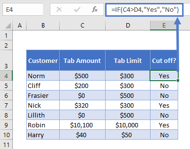
You run a sports bar and you set individual tab limits for different customers. You’ve set up this spreadsheet to check if each customer is over their limit, in which case you’ll cut them off until they pay their tab.
You check if C4-D4 (their current tab amount minus their limit), is greater than 0. This is your logical test. If this is true, IF returns “Yes” – you should cut them off. If this is false, IF returns “No” – you let them keep drinking.
What can IF Return?
Above we returned a text string, “Yes” or “No”. But you can also return numbers, or even other formulas.
Let’s say some of your customers are running up big tabs. To discourage this, you’re going to start charging interest on customers who go over their limit.
You can use IF for that:
=IF(C4>D4,C4*0.03,0)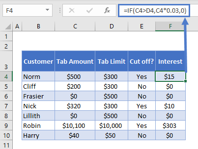
If the tab is higher than the limit, return the tab multiplied by 0.03, which returns 3% of the tab. Otherwise, return 0: they aren’t over their tab, so you won’t charge interest.
Using IF with AND
You can combine IF with Excel’s AND Function to test more than one condition. Excel will only return TRUE if ALL of the tests are true.
So, you implemented your interest rate. But some of your regulars are complaining. They’ve always paid their tabs in the past, why are you cracking down on them now? You come up with a solution: you won’t charge interest to certain trusted customers.
You make a new column to your spreadsheet to identify trusted customers, and update your IF statement with an AND function:
=IF(AND(C4>D4, F4="No"),C4*0.03,0)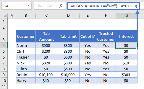
Let’s look at the AND part separately:
AND(C4>D4, F4="No")Note the two conditions:
- C4>D4: checking if they’re over their tab limit, as before
- F4=”No”: this is the new bit, checking if they are not a trusted customer
So now we only return the interest rate if the customer is over their tab, AND we have “No” in the trusted customer column. Your regulars are happy again.
Using IF with OR
The OR Function allows you to test more than one condition, returning TRUE if any conditions are met.
Maybe customers being over their tab is not the only reason you’d cut them off. Maybe you give some people a temporary ban for other reasons, gambling on the premises perhaps.
So you add a new column to identify banned customers, and update your “Cut off?” column with an OR test:
=IF(OR(C4>D4,E4="Yes"),"Yes","No")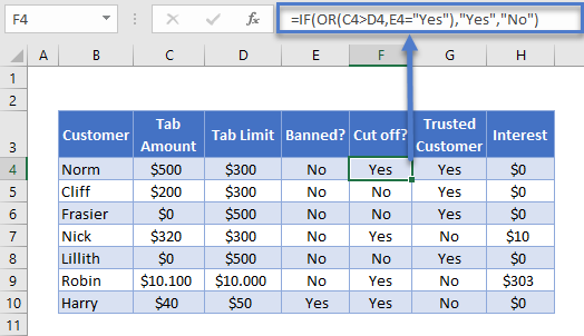
Looking just at the OR part:
OR(C4>D4,E4="Yes")There are two conditions:
- C4>D4: checking if they’re over their tab limit
- F4=”Yes”: the new part, checking if they are currently banned
This will evaluate to true if they are over their tab, or if there is a “Yes” in column E. As you can see, Harry is cut off now, even though he’s not over his tab limit.
Using IF with XOR
The XOR Function returns TRUE if only one condition is met. If more than one condition is met (or not conditions are met). It returns FALSE.
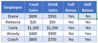
An example might make this clearer. Imagine you want to start giving monthly bonuses to your staff :
- If they sell over $800 in food, or over $800 in drinks, you’ll give them a half bonus
- If they sell over $800 in both, you’ll give them a full bonus
- If they sell under $800 in both, they don’t get any bonus.
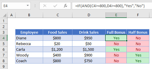
You already know how to work out if they get the full bonus. You’d just use IF with AND, as described earlier.
=IF(AND(C4>800,D4>800),"Yes","No")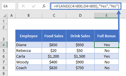
But how would you work out who gets the half bonus? That’s where XOR comes in:
=IF(XOR(C4>=800,D4>=800),"Yes","No")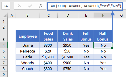
As you can see, Woody’s drink sales were over $800, but not food sales. So he gets the half bonus. The reverse is true for Coach. Diane and Carla sold more than $800 for both, so they don’t get a half bonus (both arguments are TRUE), and Rebecca made under the threshold for both (both arguments FALSE), so the formula again returns “No”.
Using IF with NOT
The NOT Function reverses the outcome of a logical test. In other words, it checks whether a condition has not been met.
You can use it with IF like this:
=IF(AND(C3>=1985,NOT(D3="Steven Spielberg")),"Watch", "Don’t Watch")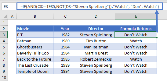
Here we have a table with data on some 1980s movies. We want to identify movies released on or after 1985, that were not directed by Steven Spielberg.
Because NOT is nested within an AND Function, Excel will evaluate that first. It will then use the result as part of the AND.
Nested IF Statements
You can also return an IF statement within your IF statement. This enables you to make more complex calculations.
Let’s go back to our customers table. Imagine you want to classify customers based on their debt level to you:
- $0: None
- Up to $500: Low
- $500 to $1000: Medium
- Over $1000: High
You can do this by “nesting” IF statements:
=IF(C4=0,"None",IF(C4<=500,"Low",IF(C4<=1000,"Medium",IF(C4>1000,"High"))))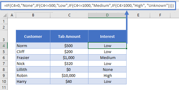
It’s easier to understand if you put the IF statements on separate lines (ALT + ENTER on Windows, CTRL + COMMAND + ENTER on Macs):
=
IF(C4=0,"None",
IF(C4<=500,"Low",
IF(C4<=1000,"Medium",
IF(C4>1000,"High", "Unknown"))))
IF C4 is 0, we return “None”. Otherwise, we move to the next IF statement. IF C4 is equal to or less than 500, we return “Low”. Otherwise, we move on to the next IF statement… and so on.
Simplifying Complex IF Statements with Helper Columns
If you have multiple nested IF statements, and you’re throwing in logic functions too, your formulas can become very hard to read, test, and update.
This is especially important to keep in mind if other people will be using the spreadsheet. What makes sense in your head, might not be so obvious to others.
Helper columns are a great way around this issue.
You’re an analyst in the finance department of a large corporation. You’ve been asked to create a spreadsheet that checks whether each employee is eligible for the company pension.
Here’s the criteria:
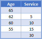
So if you’re under the age of 55, you need to have 30 years’ service under your belt to be eligible. If you’re aged 55 to 59, you need 15 years’ service. And so on, up to age 65, where you’re eligible no matter how long you’ve worked there.
You could use a single, complex IF statement to solve this problem:
=IF(OR(F4>=65,AND(F4>=62,G4>=5),AND(F4>=60,G4>=10),AND(F4>=55,G4>=15),G4>30),"Eligible", "Not Eligible")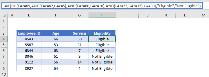
Whew! Kinda hard to get your head around that, isn’t it?
A better approach might be to use helper columns. We have five logical tests here, corresponding to each row in the criteria table. This is easier to see if we add line breaks to the formula, as we discussed earlier:
=IF(
OR(
F4>=65,
AND(F4>=62,G4>=5),
AND(F4>=60,G4>=10),
AND(F4>=55,G4>=15),
G4>30
),"Eligible","Not Eligible")
So, we can split these five tests into separate columns, and then simply check whether any one of them is true:
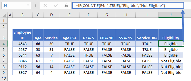
Each column in the table from E to I holds each of our criteria separately. Then in J4 we have the following formula:
=IF(COUNTIF(E4:I4,TRUE),"Eligible","Not Eligible")Here we have an IF statement, and the logical test uses COUNTIF to count the number of cells within E4:I4 that contain TRUE.
If COUNTIF doesn’t find a TRUE value, it will return 0, which IF interprets as FALSE, so the IF returns “Not Eligible”.
If COUNTIF does find any TRUE values, it will return the number of them. IF interprets any number other than 0 as TRUE, so it returns “Eligible”.
Splitting out the logical tests in this way makes the formula easier to read, and if something’s going wrong with it, it’s much easier to spot where the mistake is.
Using Grouping to Hide Helper Columns
Helper columns make the formula easier to manage, but once you’ve got them in place and you know they are working correctly, they often just take up space on your spreadsheet without adding any useful information.
You could hide the columns, but this can lead to problems because hidden columns are hard to detect, unless you look closely at the column headers.
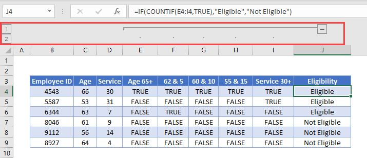
A better option is grouping.
Select the columns you want to group, in our case E:I. Then press ALT + SHIFT + RIGHT ARROW on Windows, or COMMAND + SHIFT + K on Mac. You can also go to the “Data” tab on the ribbon and select “Group” from the “Outline” section.
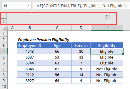
You’ll see the group displayed above the column headers, like this:
Then simply press the “-“ button to hide the columns:
The IFS Function
Nested IF statements are very useful when you need to perform more complex logical comparisons, and you need to do it in one cell. However, they can get complicated as they get longer, and they can be hard to read and update on your screen.
From Excel 2019 and Excel 365, Microsoft introduced another function, the IFS Function, to help make this a bit easier to manage. The nested IF example above could be achieved with IFS like this:
=IFS(
C4=0,"None",
C4<=500,"Low",
C4<=1000,"Medium",
C4>1000,"High",
TRUE, "Unknown",
)
You can read all about it on the main page for the Excel IFS Function <<link>>.
Using IF with Conditional Formatting
Excel’s Conditional Formatting feature enables you to format a cell in different ways depending on its contents. Since the IF returns different values based on our logical test, we might want to use Conditional Formatting with the IF Function to make these different values easier to see.
So let’s go back to our staff bonus table from earlier.
We’re returning “Yes” or “No” depending on what bonus we want to give. This tells us what we need to know, but the information doesn’t jump out at us. Let’s try to fix that.
Here’s how you’d do it:
- Select the cell range containing your IF statements. In our case that’s E4:F8.
- Click “Conditional Formatting” on the “Styles” section of the “Home” tab on the ribbon.
- Click “Highlight Cells Rules” and then “Equal to”.
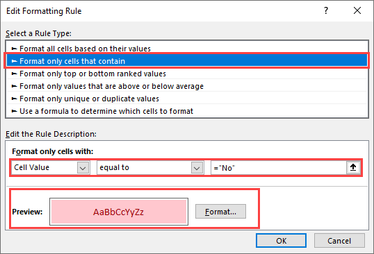
- Type “Yes” (or whatever return value you need) into the first box, and then choose the formatting you want from the second box. (I’ll choose green for this).
- Repeat for all your return values (I’ll also set “No” values to red)
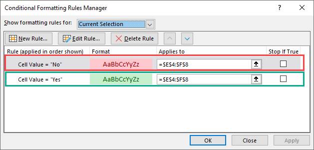
Here’s the result:
Using IF in Array Formulas
An array is a range of values, and in Excel arrays are represented as comma separated values enclosed in braces, such as:
{1,2,3,4,5}The beauty of arrays, is that they enable you to perform a calculation on each value in the range, and then return the result. For example, the SUMPRODUCT Function takes two arrays, multiplies them together, and sums the results.
So this formula:
=SUMPRODUCT({1,2,3},{4,5,6})…returns 32. Why? Let’s work it through:
1 * 4 = 4
2 * 5 = 10
3 * 6 = 18

4 + 10 + 18 = 32
We can bring an IF statement into this picture, so that each of these multiplications only happens if a logical test returns true.
For example, take this data:
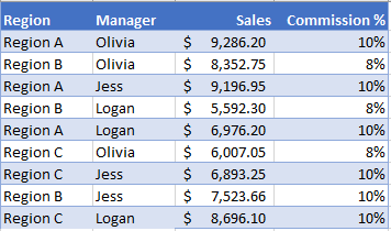
If you wanted to calculate the total commission for each sales manager, you’d use the following:
=SUMPRODUCT(IF($C$2:$C$10=$G2,$D$2:$D$10*$E$2:$E$10))Note: In Excel 2019 and earlier, you have to press CTRL + SHIFT + ENTER to turn this into an array formula.
We’d end up with something like this:
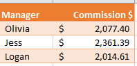
Breaking this down, the “Manager” column is column C, and in this example, Olivia’s name is in G2.
So the logical test is:
$C$2:$C$10=$G2In English, if the name in column C is equal to what’s in G2 (“Olivia”), DO multiply the values in columns D and E for that row. Otherwise, don’t multiply them. Then, sum all the results.
You can learn more about this formula on the main page for the SUMPRODUCT IF Formula.
IF in Google Sheets
The IF Function works exactly the same in Google Sheets as in Excel:
VBA IF Statements
You can also use If Statements in VBA. Click the link to learn more, but here is a simple example:
Sub Test_IF ()

If Range("a1").Value < 0 then
  Range("b1").Value = "Negative"
End If

End Sub
This code will test if a cell value is negative. If so, it will write “negative” in the next cell.
Basic logical test in Excel
In Excel, any logical test returns TRUE of FALSE.
For instance, to compare the contains of 2 columns, you have to write the following test.
=A2=B2

In this second example, we want to know if our customer have 21 years-old or more. So we create the following test with an absolute reference to the limit cell.
=B2>=$G$4

How to convert the test to a numeric value?
So when you create a test in Excel, the result is TRUE or FALSE by default.
Tips 💡And the result is always displayed in the center of the cell, ALWAYS 😉
But, you can convert TRUE or FALSE to 1 or 0 with 2 different method
Method 1: Multiply by 1
The first method is to multiply the logical test by 1
=(logical test)*1

You can see in column D the formula used
Method 2: Write 2 dashes
The other technique is to write 2 dashes before the test like in this example.
=—(logical test)

And the result is the same; the test returns 0 or 1.
The logical IF statement in Excel is used for the recording of certain conditions. It compares the number and / or text, function, etc. of the formula when the values correspond to the set parameters, and then there is one record, when do not respond — another.
Logic functions — it is a very simple and effective tool that is often used in practice. Let us consider it in details by examples.
The syntax of the function «IF» with one condition
The operation syntax in Excel is the structure of the functions necessary for its operation data.
=IF(boolean;value_if_TRUE;value_if_FALSE)
Let us consider the function syntax:
- Boolean – what the operator checks (text or numeric data cell).
- Value_if_TRUE – what will appear in the cell when the text or numbers correspond to a predetermined condition (true).
- Value_if_FALSE – what appears in the box when the text or the number does not meet the predetermined condition (false).
Example:

Logical IF functions.
The operator checks the A1 cell and compares it to 20. This is a «Boolean». When the contents of the column is more than 20, there is a true legend «greater 20». In the other case it’s «less or equal 20».
Attention! The words in the formula need to be quoted. For Excel to understand that you want to display text values.
Here is one more example. To gain admission to the exam, a group of students must successfully pass a test. The results are listed in a table with columns: a list of students, a credit, an exam.

The statement IF should check not the digital data type but the text. Therefore, we prescribed in the formula В2= «done» We take the quotes for the program to recognize the text correctly.
The function IF in Excel with multiple conditions
Usually one condition for the logic function is not enough. If you need to consider several options for decision-making, spread operators’ IF into each other. Thus, we get several functions IF in Excel.
The syntax is as follows:
Here the operator checks the two parameters. If the first condition is true, the formula returns the first argument is the truth. False — the operator checks the second condition.
Examples of a few conditions of the function IF in Excel:

It’s a table for the analysis of the progress. The student received 5 points:
- А – excellent;
- В – above average or superior work;
- C – satisfactory;
- D – a passing grade;
- E – completely unsatisfactory.
IF statement checks two conditions: the equality of value in the cells.

In this example, we have added a third condition, which implies the presence of another report card and «twos». The principle of the operator is the same.
Enhanced functionality with the help of the operators «AND» and «OR»
When you need to check out a few of the true conditions you use the function И. The point is: IF A = 1 AND A = 2 THEN meaning в ELSE meaning с.
OR function checks the condition 1 or condition 2. As soon as at least one condition is true, the result is true. The point is: IF A = 1 OR A = 2 THEN value B ELSE value C.
Functions AND & OR can check up to 30 conditions.
An example of using the operator AND:

It’s the example of using the logical operator OR.

How to compare data in two tables
Users often need to compare the two spreadsheets in an Excel to match. Examples of the «life»: compare the prices of goods in different bringing, to compare balances (accounting reports) in a few months, the progress of pupils (students) of different classes, in different quarters, etc.
To compare the two tables in Excel, you can use the COUNTIFS statement. Consider the order of application functions.
For example, consider the two tables with the specifications of various food processors. We planned allocation of color differences. This problem in Excel solves the conditional formatting.
Baseline data (tables, which will work with):

Select the first table. Conditional Formatting — create a rule — use a formula to determine the formatted cells:

In the formula bar write: = COUNTIFS (comparable range; first cell of first table)=0. Comparing range is in the second table.
To drive the formula into the range, just select it first cell and the last. «= 0» means the search for the exact command (not approximate) values.
Choose the format and establish what changes in the cell formula in compliance. It’s better to do a color fill.
Select the second table. Conditional Formatting — create a rule — use the formula. Use the same operator (COUNTIFS). For the second table formula:
Download all examples in Excel

Now it is easy to compare the characteristics of the data in the table.