
IF function
The IF function is one of the most popular functions in Excel, and it allows you to make logical comparisons between a value and what you expect.
So an IF statement can have two results. The first result is if your comparison is True, the second if your comparison is False.
For example, =IF(C2=”Yes”,1,2) says IF(C2 = Yes, then return a 1, otherwise return a 2).

Use the IF function, one of the logical functions, to return one value if a condition is true and another value if it’s false.
IF(logical_test, value_if_true, [value_if_false])
For example:
-
=IF(A2>B2,»Over Budget»,»OK»)
-
=IF(A2=B2,B4-A4,»»)
|
Argument name |
Description |
|---|---|
|
logical_test (required) |
The condition you want to test. |
|
value_if_true (required) |
The value that you want returned if the result of logical_test is TRUE. |
|
value_if_false (optional) |
The value that you want returned if the result of logical_test is FALSE. |
Simple IF examples

-
=IF(C2=”Yes”,1,2)
In the above example, cell D2 says: IF(C2 = Yes, then return a 1, otherwise return a 2)

-
=IF(C2=1,”Yes”,”No”)
In this example, the formula in cell D2 says: IF(C2 = 1, then return Yes, otherwise return No)As you see, the IF function can be used to evaluate both text and values. It can also be used to evaluate errors. You are not limited to only checking if one thing is equal to another and returning a single result, you can also use mathematical operators and perform additional calculations depending on your criteria. You can also nest multiple IF functions together in order to perform multiple comparisons.

-
=IF(C2>B2,”Over Budget”,”Within Budget”)
In the above example, the IF function in D2 is saying IF(C2 Is Greater Than B2, then return “Over Budget”, otherwise return “Within Budget”)

-
=IF(C2>B2,C2-B2,0)
In the above illustration, instead of returning a text result, we are going to return a mathematical calculation. So the formula in E2 is saying IF(Actual is Greater than Budgeted, then Subtract the Budgeted amount from the Actual amount, otherwise return nothing).

-
=IF(E7=”Yes”,F5*0.0825,0)
In this example, the formula in F7 is saying IF(E7 = “Yes”, then calculate the Total Amount in F5 * 8.25%, otherwise no Sales Tax is due so return 0)
Note: If you are going to use text in formulas, you need to wrap the text in quotes (e.g. “Text”). The only exception to that is using TRUE or FALSE, which Excel automatically understands.
Common problems
|
Problem |
What went wrong |
|---|---|
|
0 (zero) in cell |
There was no argument for either value_if_true or value_if_False arguments. To see the right value returned, add argument text to the two arguments, or add TRUE or FALSE to the argument. |
|
#NAME? in cell |
This usually means that the formula is misspelled. |
Need more help?
You can always ask an expert in the Excel Tech Community or get support in the Answers community.

See Also
IF function — nested formulas and avoiding pitfalls
IFS function
Using IF with AND, OR and NOT functions
COUNTIF function
How to avoid broken formulas
Overview of formulas in Excel
Need more help?
Want more options?
Explore subscription benefits, browse training courses, learn how to secure your device, and more.
Communities help you ask and answer questions, give feedback, and hear from experts with rich knowledge.
Содержание
- IFS function
- Simple syntax
- Example 1
- Example 2
- Remarks
- Need more help?
- IF function – nested formulas and avoiding pitfalls
- Remarks
- Examples
- Additional examples
- Did you know?
- Need more help?
- Excel IF Function – How to Use
- Definition of Excel IF Function
- Syntax
- Important Characteristics of IF Function in Excel
- Comparison Operators That Can Be Used With IF Statements
- Example 1: Using ‘equal to’ comparison operator within the IF function
- Example 2: Using ‘not equal to’ comparison operator within the IF function.
- Example 3: Using ‘less than’ operator within the IF function.
- Example 4: Using ‘greater than or equal to’ operator within the IF statement.
- Example 5: Using ‘greater than’ operator within the IF statement.
- Example 6: Using ‘less than or equal to’ operator within the IF statement.
- Example 7: Using an Excel Logical Function within the IF formula in Excel.
- Example 8: Using the Excel IF function to return another formula a result.
- Use Of AND & OR Functions or Logical Operators with Excel IF Statement
- Example 9: Using the IF function along with AND Function.
- Example 10: Using the IF function along with OR Function.
- Nested IF Statements
- Syntax:
- The above syntax translates to this:
- Example 11: Nested IF Statements
- Partial Matching or Wildcards with IF Function
- Example 12: Using FIND and SEARCH functions inside the IF statement
- Example 13: Using SEARCH function inside the Excel IF formula with wildcard operators
- Some Practical Examples of using the IF function
- Example 14: Using Excel IF function with dates.
- Example 15: Use an IF function-based formula to find blank cells in excel.
- Example 16: Use the Excel IF statement to show symbolic results (instead of textual results).
- IFS Function In Excel:
- Syntax for IFS function:
- Example 17: Using IFS function in Excel
- Subscribe and be a part of our 15,000+ member family!
IFS function
The IFS function checks whether one or more conditions are met, and returns a value that corresponds to the first TRUE condition. IFS can take the place of multiple nested IF statements, and is much easier to read with multiple conditions.
Note: This feature is available on Windows or Mac if you have Office 2019, or if you have a Microsoft 365 subscription. If you are a Microsoft 365 subscriber, make sure you have the latest version.
Simple syntax
Generally, the syntax for the IFS function is:
=IFS([Something is True1, Value if True1,Something is True2,Value if True2,Something is True3,Value if True3)
Please note that the IFS function allows you to test up to 127 different conditions. However, we don’t recommend nesting too many conditions with IF or IFS statements. This is because multiple conditions need to be entered in the correct order, and can be very difficult to build, test and update.
IFS(logical_test1, value_if_true1, [logical_test2, value_if_true2], [logical_test3, value_if_true3],…)
Condition that evaluates to TRUE or FALSE.
Result to be returned if logical_test1 evaluates to TRUE. Can be empty.
Condition that evaluates to TRUE or FALSE.
Result to be returned if logical_testN evaluates to TRUE. Each value_if_trueN corresponds with a condition logical_testN. Can be empty.
Example 1
The formula for cells A2:A6 is:
Which says IF(A2 is Greater Than 89, then return a «A», IF A2 is Greater Than 79, then return a «B», and so on and for all other values less than 59, return an «F»).
Example 2
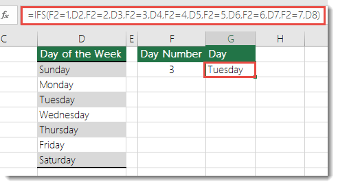
The formula in cell G7 is:
Which says IF(the value in cell F2 equals 1, then return the value in cell D2, IF the value in cell F2 equals 2, then return the value in cell D3, and so on, finally ending with the value in cell D8 if none of the other conditions are met).
To specify a default result, enter TRUE for your final logical_test argument. If none of the other conditions are met, the corresponding value will be returned. In Example 1, rows 6 and 7 (with the 58 grade) demonstrate this.
If a logical_test argument is supplied without a corresponding value_if_true, this function shows a «You’ve entered too few arguments for this function» error message.
If a logical_test argument is evaluated and resolves to a value other than TRUE or FALSE, this function returns a #VALUE! error.
If no TRUE conditions are found, this function returns #N/A error.
Need more help?
You can always ask an expert in the Excel Tech Community or get support in the Answers community.
Источник
IF function – nested formulas and avoiding pitfalls
The IF function allows you to make a logical comparison between a value and what you expect by testing for a condition and returning a result if True or False.
=IF(Something is True, then do something, otherwise do something else)
So an IF statement can have two results. The first result is if your comparison is True, the second if your comparison is False.
IF statements are incredibly robust, and form the basis of many spreadsheet models, but they are also the root cause of many spreadsheet issues. Ideally, an IF statement should apply to minimal conditions, such as Male/Female, Yes/No/Maybe, to name a few, but sometimes you might need to evaluate more complex scenarios that require nesting* more than 3 IF functions together.
* “Nesting” refers to the practice of joining multiple functions together in one formula.
Use the IF function, one of the logical functions, to return one value if a condition is true and another value if it’s false.
IF(logical_test, value_if_true, [value_if_false])
The condition you want to test.
The value that you want returned if the result of logical_test is TRUE.
The value that you want returned if the result of logical_test is FALSE.
While Excel will allow you to nest up to 64 different IF functions, it’s not at all advisable to do so. Why?
Multiple IF statements require a great deal of thought to build correctly and make sure that their logic can calculate correctly through each condition all the way to the end. If you don’t nest your formula 100% accurately, then it might work 75% of the time, but return unexpected results 25% of the time. Unfortunately, the odds of you catching the 25% are slim.
Multiple IF statements can become incredibly difficult to maintain, especially when you come back some time later and try to figure out what you, or worse someone else, was trying to do.
If you find yourself with an IF statement that just seems to keep growing with no end in sight, it’s time to put down the mouse and rethink your strategy.
Let’s look at how to properly create a complex nested IF statement using multiple IFs, and when to recognize that it’s time to use another tool in your Excel arsenal.
Examples
Following is an example of a relatively standard nested IF statement to convert student test scores to their letter grade equivalent.
 97,»A+»,IF(B2>93,»A»,IF(B2>89,»A-«,IF(B2>87,»B+»,IF(B2>83,»B»,IF(B2>79,»B-«,IF(B2>77,»C+»,IF(B2>73,»C»,IF(B2>69,»C-«,IF(B2>57,»D+»,IF(B2>53,»D»,IF(B2>49,»D-«,»F»))))))))))))» loading=»lazy»>
This complex nested IF statement follows a straightforward logic:
If the Test Score (in cell D2) is greater than 89, then the student gets an A
If the Test Score is greater than 79, then the student gets a B
If the Test Score is greater than 69, then the student gets a C
If the Test Score is greater than 59, then the student gets a D
Otherwise the student gets an F
This particular example is relatively safe because it’s not likely that the correlation between test scores and letter grades will change, so it won’t require much maintenance. But here’s a thought – what if you need to segment the grades between A+, A and A- (and so on)? Now your four condition IF statement needs to be rewritten to have 12 conditions! Here’s what your formula would look like now:
It’s still functionally accurate and will work as expected, but it takes a long time to write and longer to test to make sure it does what you want. Another glaring issue is that you’ve had to enter the scores and equivalent letter grades by hand. What are the odds that you’ll accidentally have a typo? Now imagine trying to do this 64 times with more complex conditions! Sure, it’s possible, but do you really want to subject yourself to this kind of effort and probable errors that will be really hard to spot?
Tip: Every function in Excel requires an opening and closing parenthesis (). Excel will try to help you figure out what goes where by coloring different parts of your formula when you’re editing it. For instance, if you were to edit the above formula, as you move the cursor past each of the ending parentheses “)”, its corresponding opening parenthesis will turn the same color. This can be especially useful in complex nested formulas when you’re trying to figure out if you have enough matching parentheses.
Additional examples
Following is a very common example of calculating Sales Commission based on levels of Revenue achievement.
 15000,20%,IF(C9>12500,17.5%,IF(C9>10000,15%,IF(C9>7500,12.5%,IF(C9>5000,10%,0)))))» loading=»lazy»>
This formula says IF(C9 is Greater Than 15,000 then return 20%, IF(C9 is Greater Than 12,500 then return 17.5%, and so on.
While it’s remarkably similar to the earlier Grades example, this formula is a great example of how difficult it can be to maintain large IF statements – what would you need to do if your organization decided to add new compensation levels and possibly even change the existing dollar or percentage values? You’d have a lot of work on your hands!
Tip: You can insert line breaks in the formula bar to make long formulas easier to read. Just press ALT+ENTER before the text you want to wrap to a new line.
Here is an example of the commission scenario with the logic out of order:
 5000,10%,IF(C9>7500,12.5%,IF(C9>10000,15%,IF(C9>12500,17.5%,IF(C9>15000,20%,0)))))» loading=»lazy»>
Can you see what’s wrong? Compare the order of the Revenue comparisons to the previous example. Which way is this one going? That’s right, it’s going from bottom up ($5,000 to $15,000), not the other way around. But why should that be such a big deal? It’s a big deal because the formula can’t pass the first evaluation for any value over $5,000. Let’s say you’ve got $12,500 in revenue – the IF statement will return 10% because it is greater than $5,000, and it will stop there. This can be incredibly problematic because in a lot of situations these types of errors go unnoticed until they’ve had a negative impact. So knowing that there are some serious pitfalls with complex nested IF statements, what can you do? In most cases, you can use the VLOOKUP function instead of building a complex formula with the IF function. Using VLOOKUP, you first need to create a reference table:

This formula says to look for the value in C2 in the range C5:C17. If the value is found, then return the corresponding value from the same row in column D.

Similarly, this formula looks for the value in cell B9 in the range B2:B22. If the value is found, then return the corresponding value from the same row in column C.
Note: Both of these VLOOKUPs use the TRUE argument at the end of the formulas, meaning we want them to look for an approxiate match. In other words, it will match the exact values in the lookup table, as well as any values that fall between them. In this case the lookup tables need to be sorted in Ascending order, from smallest to largest.
VLOOKUP is covered in much more detail here, but this is sure a lot simpler than a 12-level, complex nested IF statement! There are other less obvious benefits as well:
VLOOKUP reference tables are right out in the open and easy to see.
Table values can be easily updated and you never have to touch the formula if your conditions change.
If you don’t want people to see or interfere with your reference table, just put it on another worksheet.
Did you know?
There is now an IFS function that can replace multiple, nested IF statements with a single function. So instead of our initial grades example, which has 4 nested IF functions:
It can be made much simpler with a single IFS function:
The IFS function is great because you don’t need to worry about all of those IF statements and parentheses.
Note: This feature is only available if you have a Microsoft 365 subscription. If you are a Microsoft 365subscriber, make sure you have the latest version of Office.
Need more help?
You can always ask an expert in the Excel Tech Community or get support in the Answers community.
Источник
Excel IF Function – How to Use
IF function is undoubtedly one of the most important functions in excel. In general, IF statements give the desired intelligence to a program so that it can make decisions based on given criteria and, most importantly, decide the program flow.
In Microsoft Excel terminology, IF statements are also called «Excel IF-Then statements». IF function evaluates a boolean/logical expression and returns one value if the expression evaluates to ‘TRUE’ and another value if the expression evaluates to ‘FALSE’.
Table of Contents
Definition of Excel IF Function
According to Microsoft Excel, IF function is defined as a formula which «checks whether a condition is met, returns one value if true and another value if false».
Syntax
Syntax of IF function in Excel is as follows:
‘logic_test’ (required argument) – Refers to the boolean expression or logical expression that needs to be evaluated.
‘value_if_true’ (optional argument) – Refers to the value that will be returned by the IF function if the ‘logic_test’ evaluates to TRUE.
‘value_if_false’ (optional argument) – Refers to the value that will be returned by the IF function if the ‘logic_test’ evaluates to FALSE.

Important Characteristics of IF Function in Excel
- To use the IF function, you need to provide the ‘logic_test’ or conditional statement mandatorily.
- The arguments ‘value_if_true’ and ‘value_if_false’ are optional, but you need to provide at least one of them.
- The result of the IF statement can only be any one of the two given values (either it will be ‘value_if_true’ or ‘value_if_false’ ). Both values cannot be returned at the same time.
- IF function throws a ‘#Name?’ error if the ‘logic_test’ or boolean expression you are trying to evaluate is invalid.
- Nesting of IF statements is possible, but Excel only allows this to 64 levels. Nesting of IF statement means using one if statement within another.
Comparison Operators That Can Be Used With IF Statements
Following comparison operators can be used within the ‘logic_test’ argument of the IF function:
- = (equal to)
- <> (not equal to)
- (greater than)
- >= (greater than or equal to)
- Simple Examples of Excel IF Statement
Now, let’s try to see a simple example of the Excel IF function:
Example 1: Using ‘equal to’ comparison operator within the IF function
In this example, we have a list of colors, and we aim to find the ‘Blue’ color. If we are able to find the ‘Blue’ color, then in the adjacent cell, we need to assign a ‘Yes’; otherwise, assign a ‘No’.

So, the formula would be:
This suggests that if the value present in cell A2 is ‘Blue’, then return a ‘Yes’; otherwise, return a ‘No’.
If we drag this formula down to all the rows, we will find that it returns ‘Yes’ for the cells with the value ‘Blue’ for all others; it would result in ‘No’.
Example 2: Using ‘not equal to’ comparison operator within the IF function.
Let’s take example 1, and understand how we can reverse the logic and use a ‘not equal to’ operator to construct the formula so that it still results in ‘Yes’ for ‘Blue’ color and ‘No’ for any other text.

So the formula would be:
This suggests that if the value at A2 is not equal to ‘Blue’, then return a ‘No’; otherwise, return a ‘Yes’.
When dragged down to all the below rows, this formula would find all the cells (from A2 to A8) where the value is not ‘Blue’ and marks a ‘No’ against them. Otherwise, it marks a ‘Yes’ in the adjacent cells.
Example 3: Using ‘less than’ operator within the IF function.
In this example, we have scores of some students, along with their names. We want to assign either «Pass» or «Fail» against each student in the result column.

Based on our criteria, the passing score is 50 or more.
For this, we can use the IF function as:
This suggests that if the value at B2, i.e., 37, is less than 50, then return «Fail»; otherwise, return «Pass».
As 37 is less than 50 so the result will be «Fail».
We can drag the above-given formula for the rest of the cells below and the result would be correct.
Example 4: Using ‘greater than or equal to’ operator within the IF statement.
Let’s take example 3 and see how we can reverse the logic and use a ‘greater than or equal to’ operator to construct the formula so that it still results in ‘Pass’ for scores of 50 or more and ‘Fail’ for all the other scores.

For this, we can use the Excel IF function as:
This suggests that if the value at B2, i.e., 37 is greater than or equal to 50, then return «Pass»; otherwise, return «Fail».
As 37 not greater than or equal to 50 so the result will be «Fail».
When dragged down for the rest of the cells below, this formula would assign the correct result in the adjacent rows.
Example 5: Using ‘greater than’ operator within the IF statement.
In this example, we have a small online store that gives a discount to its customers based on the amount they spend. If a customer spends $50 or more, he is applicable for a 5% discount; otherwise, no discounts are offered.

To find whether a discount is offered or not, we can use the following excel formula:
This translates to – If the value at B2 cell is greater than 50, assign a text «5% Discount» otherwise, assign a text «No Discount» against the customer.
In the first case, as 23 is not greater than 50, the output will be «No Discount».
We can drag the above-given formula for the rest of the cells below are the result would be correct.
Example 6: Using ‘less than or equal to’ operator within the IF statement.
Let’s take example 5 and see how we can reverse the logic and use a ‘less than or equal to’ operator to construct the formula so that it still results in a ‘5% Discount’ for all customers whose total spend exceeds $50 and ‘No Discount’ for all the other customers.

For this, we can use the IF-then statement as:
This means that if the value at B2, i.e., 23, is less than or equal to 50, then return «No Discount»; otherwise, return «5% Discount».
As 23 is less than or equal to 50 so the result will be «No Discount».
When dragged down for the rest of the cells below, this formula would assign the correct result in the adjacent rows.
Example 7: Using an Excel Logical Function within the IF formula in Excel.
In this example, let’s suppose we have a list of numbers, and we have to mark Even and Odd numbers. We can do this using the IF condition and the ISEVEN or ISODD inbuilt functions provided by Microsoft Excel.
ISEVEN function returns ‘true’ if the number passed to it is even; otherwise, it returns a ‘false’. Similarly, ISODD function return ‘true’ if the number passed to it is odd; otherwise, it returns a ‘false’.

For this, we can use the IF-then statement as:
This means that – If the value at A2 cell is an even number, then the result would be «Even»; otherwise, the result would be «Odd».
Alternatively, the above logic can also be written using the ISODD function along with the IF statement as:
This means that – If the value at A2 cell is an odd number, then the result would be «Odd»; otherwise, the result would be «Even».
Example 8: Using the Excel IF function to return another formula a result.
In this example, we have Employee Data from a company. The company comes up with a simple way to reward its loyal employees. They decide to give the employees an annual bonus based on the years spent by the employee within the organization.
Employees with experience of more than 5 years are given 10% of annual salary as a bonus whereas everyone else gets a 5% of annual salary as a bonus.

For this, the excel formula would be:
This means that – if the value at B2 (experience column) is greater than 5, then return a result by calculating 10% of C2 (annual salary column). However, if the logic test is evaluated to false, then return the result by calculating 5% of C2 (annual salary column)
Use Of AND & OR Functions or Logical Operators with Excel IF Statement
Excel IF Statement can also be used along with the other functions like AND, OR, NOT for analyzing complex logic. These functions (AND, OR & NOT) are called logical operators as they are used for connecting two or more logical expressions.
AND Function– AND function returns true when all the conditions inside the AND function evaluate to true. The syntax of AND Function in Excel is:
OR Function– OR function returns true when any one of the conditions inside the OR function evaluates to true. The syntax of OR Function in Excel is:
Example 9: Using the IF function along with AND Function.
In this example, we have Math and science test scores of some students, and we want to assign a ‘Pass’ or ‘Fail’ value against the students based on their scores.
Passing criteria: Students have to get more than 50 marks in Math and more than 70 marks in science to pass the test.

Based on the above conditions, the formula would be:
The formula translates to – if the value at B2 (Math score) is greater than 50 and the value at C2 (Science Score) is greater than 70, then assign the value «Pass»; otherwise, assign the value «Fail».
Example 10: Using the IF function along with OR Function.
In this example, we have two test scores of some students, and we want to assign a ‘Pass’ or ‘Fail’ value against the students based on their scores.
Passing criteria: Students have to clear either one of the two tests with more than 50 marks.

Based on the above conditions, the formula would be:
The formula translates to – if either the value at B2 (Test 1 score) is greater than 50, OR the value at C2 (Test 2 Score) is greater than 50, then assign the value «Pass»; otherwise, assign the value «Fail».
Nested IF Statements
When used alone, IF formula can only result in two outcomes, i.e., True or False. But there are many cases when we want to test multiple outcomes with IF statement.
In such cases, nesting two or more IF Then statements one inside another can be convenient in writing formulas.
Syntax:
The syntax of the Nested IF Then statements is as follows:
‘condition_1’ – Refers to the first logical test or conditional expression that needs to be evaluated by the outer IF function.
‘value_if_true_1’ – Refers to the value that will be returned by the outer IF function if the ‘condition_1’ evaluates to TRUE.
‘condition_2’ – Refers to the second logical test or conditional expression that needs to be evaluated by the inner IF function.
‘value_if_true_2’ – Refers to the value that will be returned by the inner IF function if the ‘condition_2’ evaluates to TRUE.
‘value_if_false_2’ – Refers to the value that will be returned by the inner IF function if the ‘condition_2’ evaluates to FALSE.
The above syntax translates to this:
As we can see, Nested formulas can quickly become complicated so, let’s try to understand how nesting of the IF statement works with an example.
Example 11: Nested IF Statements
In this example, we have a list of countries and their average temperatures in degree Celsius for the month of January. Our goal is to categorize the country based on the temperature range as follows:
Criteria: Temperatures below 20 °C should be marked as «Below Room Temperature», temperatures between 20°C to 25°C should be classified as «Normal Room Temperature», whereas any temperature over 25°C should be marked as «Above Room Temperature».

Based on the above conditions, the formula would be:
The formula translates to – if the value at B2 is less than 20, then the text «Below Room Temperature» is returned from the outer IF block. However, if the value at B2 is greater than or equal to 20, then the inner IF block is evaluated.
Inside the inner IF block, the value at B2 is checked. If the value at B2 is greater than or equal to 20 and less than or equal to 25. Then the inner IF block returns the text «Normal Room Temperature».
However, if the condition inside the inner IF block also evaluates to ‘false’ that means the value at B2 is greater than 25, so the result will be «Above Room Temperature».
Partial Matching or Wildcards with IF Function
Although IF function itself doesn’t accept any wildcard characters like (* or ?) while performing the logic test, thankfully, there are ways to perform partial matching and wildcard searches with the IF function.
To perform partial matching inside the IF function, we can use the FIND (case sensitive) or SEARCH (case insensitive) functions.
Let’s have a look at this with some examples.
Example 12: Using FIND and SEARCH functions inside the IF statement
In this example, we have a list of customers, and we need to find all the customers whose last name is «Flynn». If the customer name contains the text «Flynn», then we need to assign a text «Found» against their names. Otherwise, we need to assign a text «Not Found».

For this, we can make use of the FIND function within the IF function as:
Using the FIND function, we perform a case-sensitive search of the text «Flynn» within the customer name column. If the FIND function is able to find the text «Flynn», it returns a number signifying the position where it found the text.
If the number returned by the FIND function is valid, the ISNUMBER Function returns a value true. Else, it returns false. Based on the ISNUMBER function’s output, the logic test is performed and the appropriate value «Found» or «Not Found» is assigned.
Note: It should be noted that the FIND function performs a case-sensitive search.
This means in the above example if the customer name is entered in lower case (like «sean flynn» then the above function would return not found against them.
To perform a case-insensitive search, we can replace the find function with the search function, and the rest of the formula would be the same.
Example 13: Using SEARCH function inside the Excel IF formula with wildcard operators
In this example, we have the same customer list from example 12, and we need to find all the customers whose name contains «M». If the customer name contains the alphabet «M», we need to assign a text «M Found» against their names. Otherwise, we need to assign a text «M Not Found».

For this, we can use the SEARCH function with a wildcard ‘*’ operator inside the IF function as:
For more details on Search Function and wildcard, operators check out this article – Search Function In Excel
Some Practical Examples of using the IF function
Now, let’s have a look at some more practical examples of the Excel IF Function.
Example 14: Using Excel IF function with dates.
In this example, we have a task list along with the task due dates. Our goal is to show results based on the task due date.
If the task due date was in the past, we need to show «Was due <1,2,3..>day(s) back», if the task due date is today’s date, we need to show «Today» and similarly, if the task due date is in the future then we need to show «Due in <1,2,3..>day(s)»

In Microsoft Excel, we can do this with the help of the IF-then statement and TODAY function, as shown below:
This means that – compare the date present in cell B2 if the date is equal to today’s date show the text «Today». If the date in cell B2 is not equal to today’s date, then the inner IF block checks if the date in B2 is greater than today’s date. If the date in cell B2 is greater than today’s date, that means the date is in the future, so show the text «Due in <1,2,3…>days».
However, if the date in cell B2 is not greater than today’s date, that means the date was in the past; in such a case, show the text «Was due <1,2,3..>day(s) back».
You can also go a step further and apply conditional formatting on the range and highlight all the cells with the text «Today!». This will help you to clearly see
Example 15: Use an IF function-based formula to find blank cells in excel.
In this example, we will use the IF function to find the blank cells in Microsoft Excel. We have a list of customers, and in between the list, some of the cells are blank. We aim to find the blank cells and add the text «blank call found!» against them.

We can do this with the help of the IF function along with the ISBLANK function. The ISBLANK function returns a true if the cell reference passed to it is blank. Otherwise, the ISBLANK function returns false.
Let’s see the formula –
This means that – If the cell at A2 is blank, then the resultant text should be «Blank cell found!», however, if the cell at A2 is not blank, then don’t show any text.
Example 16: Use the Excel IF statement to show symbolic results (instead of textual results).
In this example, we have a list of sales employees of a company along with the number of products sold by the employees in the current month. We want to show an upward arrow symbol (↑) if the employee has done more than 50 sales and a downward arrow symbol (↓) if the employee has made less than 50 sales.

To do this, we can use the formula:
This implies – If the value at B2 is greater than 50, then, as a result, show the content in cell G6 (cell containing upward arrow) and otherwise show the content at G8 (cell containing downward arrow)
If you wonder about the ‘$’ signs used in the formula, you can check out this post – Excel Absolute References . These ‘$’ symbols are used for making excel cell references absolute.
IFS Function In Excel:
IFS Function in Microsoft Excel is a great alternative to nested IF Statements. It is very similar to a switch statement. The IFS function evaluates multiple conditions passed to it and returns the value corresponding to the first condition that evaluates to true.
IFS function is a lot simple to write and read than nested IF statements. IFS function is available in Office 2019 and higher versions.
Syntax for IFS function:
‘test1’ (required argument) – Refers to the first logical test that needs to be evaluated.
‘value1’ (required argument) – Refers to the result to be returned when ‘test1’ evaluates to TRUE.
‘test2’ (optional argument) – Refers to the second logical test that needs to be evaluated
‘value2’ (optional argument) – Refers to the result to be returned when ‘test2’ evaluates to TRUE.
Example 17: Using IFS function in Excel
In this example, we have a list of students, along with their scores, and we need to assign a grade to the students based on the scores.
The grading criteria is as follows – Grade A for a score of 90 or more, Grade B for a score between 80 to 89.99, Grade C for a score between 70 to 79.99, Grade D for a score between 60 to 69.99, Grade E for a score between 60 to 59.99, Grade F for a score lower than 50.

Let’s see how easily write such a complicated formula with the IFS function:
This implies that – If B2 is greater than or equal to 90, return A. Else if B2 is greater than or equal to 80, return B. Else if B2 is greater than or equal to 70, return C. Else if B2 is greater than or equal to 60, return D. Else if B2 is greater than or equal to 50, return E. Else if B2 is less than 50, return F.
If you would try to write the same formula using nested IF statements, see how long and complicated it becomes:
So, this was all about the IF function in excel. If you want to learn more about IF function, I would recommend you to go through this article – VBA IF Statement With Examples
Subscribe and be a part of our 15,000+ member family!
Now subscribe to Excel Trick and get a free copy of our ebook «200+ Excel Shortcuts» (printable format) to catapult your productivity.
Источник
Функция ЕСЛИ в Excel — это отличный инструмент для проверки условий на ИСТИНУ или ЛОЖЬ. Если значения ваших расчетов равны заданным параметрам функции как ИСТИНА, то она возвращает одно значение, если ЛОЖЬ, то другое.
Содержание
- Что возвращает функция
- Синтаксис
- Аргументы функции
- Дополнительная информация
- Функция Если в Excel примеры с несколькими условиями
- Пример 1. Проверяем простое числовое условие с помощью функции IF (ЕСЛИ)
- Пример 2. Использование вложенной функции IF (ЕСЛИ) для проверки условия выражения
- Пример 3. Вычисляем сумму комиссии с продаж с помощью функции IF (ЕСЛИ) в Excel
- Пример 4. Используем логические операторы (AND/OR) (И/ИЛИ) в функции IF (ЕСЛИ) в Excel
- Пример 5. Преобразуем ошибки в значения “0” с помощью функции IF (ЕСЛИ)
Что возвращает функция
Заданное вами значение при выполнении двух условий ИСТИНА или ЛОЖЬ.
Синтаксис
=IF(logical_test, [value_if_true], [value_if_false]) — английская версия
=ЕСЛИ(лог_выражение; [значение_если_истина]; [значение_если_ложь]) — русская версия
Аргументы функции
- logical_test (лог_выражение) — это условие, которое вы хотите протестировать. Этот аргумент функции должен быть логичным и определяемым как ЛОЖЬ или ИСТИНА. Аргументом может быть как статичное значение, так и результат функции, вычисления;
- [value_if_true] ([значение_если_истина]) — (не обязательно) — это то значение, которое возвращает функция. Оно будет отображено в случае, если значение которое вы тестируете соответствует условию ИСТИНА;
- [value_if_false] ([значение_если_ложь]) — (не обязательно) — это то значение, которое возвращает функция. Оно будет отображено в случае, если условие, которое вы тестируете соответствует условию ЛОЖЬ.
Дополнительная информация
- В функции ЕСЛИ может быть протестировано 64 условий за один раз;
- Если какой-либо из аргументов функции является массивом — оценивается каждый элемент массива;
- Если вы не укажете условие аргумента FALSE (ЛОЖЬ) value_if_false (значение_если_ложь) в функции, т.е. после аргумента value_if_true (значение_если_истина) есть только запятая (точка с запятой), функция вернет значение “0”, если результат вычисления функции будет равен FALSE (ЛОЖЬ).
На примере ниже, формула =IF(A1> 20,”Разрешить”) или =ЕСЛИ(A1>20;»Разрешить») , где value_if_false (значение_если_ложь) не указано, однако аргумент value_if_true (значение_если_истина) по-прежнему следует через запятую. Функция вернет “0” всякий раз, когда проверяемое условие не будет соответствовать условиям TRUE (ИСТИНА).
 |
| - Если вы не укажете условие аргумента TRUE(ИСТИНА) (value_if_true (значение_если_истина)) в функции, т.е. условие указано только для аргумента value_if_false (значение_если_ложь), то формула вернет значение “0”, если результат вычисления функции будет равен TRUE (ИСТИНА);
На примере ниже формула равна =IF (A1>20;«Отказать») или =ЕСЛИ(A1>20;»Отказать»), где аргумент value_if_true (значение_если_истина) не указан, формула будет возвращать “0” всякий раз, когда условие соответствует TRUE (ИСТИНА).

Функция Если в Excel примеры с несколькими условиями
Пример 1. Проверяем простое числовое условие с помощью функции IF (ЕСЛИ)
При использовании функции ЕСЛИ в Excel, вы можете использовать различные операторы для проверки состояния. Вот список операторов, которые вы можете использовать:
Ниже приведен простой пример использования функции при расчете оценок студентов. Если сумма баллов больше или равна «35», то формула возвращает “Сдал”, иначе возвращается “Не сдал”.
Пример 2. Использование вложенной функции IF (ЕСЛИ) для проверки условия выражения
Функция может принимать до 64 условий одновременно. Несмотря на то, что создавать длинные вложенные функции нецелесообразно, то в редких случаях вы можете создать формулу, которая множество условий последовательно.
В приведенном ниже примере мы проверяем два условия.
- Первое условие проверяет, сумму баллов не меньше ли она чем 35 баллов. Если это ИСТИНА, то функция вернет “Не сдал”;
- В случае, если первое условие — ЛОЖЬ, и сумма баллов больше 35, то функция проверяет второе условие. В случае если сумма баллов больше или равна 75. Если это правда, то функция возвращает значение “Отлично”, в других случаях функция возвращает “Сдал”.
Пример 3. Вычисляем сумму комиссии с продаж с помощью функции IF (ЕСЛИ) в Excel
Функция позволяет выполнять вычисления с числами. Хороший пример использования — расчет комиссии продаж для торгового представителя.
В приведенном ниже примере, торговый представитель по продажам:
- не получает комиссионных, если объем продаж меньше 50 тыс;
- получает комиссию в размере 2%, если продажи между 50-100 тыс
- получает 4% комиссионных, если объем продаж превышает 100 тыс.
Рассчитать размер комиссионных для торгового агента можно по следующей формуле:
=IF(B2<50,0,IF(B2<100,B2*2%,B2*4%)) — английская версия
=ЕСЛИ(B2<50;0;ЕСЛИ(B2<100;B2*2%;B2*4%)) — русская версия
В формуле, использованной в примере выше, вычисление суммы комиссионных выполняется в самой функции ЕСЛИ. Если объем продаж находится между 50-100K, то формула возвращает B2 * 2%, что составляет 2% комиссии в зависимости от объема продажи.
Больше лайфхаков в нашем Telegram Подписаться
Пример 4. Используем логические операторы (AND/OR) (И/ИЛИ) в функции IF (ЕСЛИ) в Excel
Вы можете использовать логические операторы (AND/OR) (И/ИЛИ) внутри функции для одновременного тестирования нескольких условий.
Например, предположим, что вы должны выбрать студентов для стипендий, основываясь на оценках и посещаемости. В приведенном ниже примере учащийся имеет право на участие только в том случае, если он набрал более 80 баллов и имеет посещаемость более 80%.
Вы можете использовать функцию AND (И) вместе с функцией IF (ЕСЛИ), чтобы сначала проверить, выполняются ли оба эти условия или нет. Если условия соблюдены, функция возвращает “Имеет право”, в противном случае она возвращает “Не имеет право”.
Формула для этого расчета:
=IF(AND(B2>80,C2>80%),”Да”,”Нет”) — английская версия
=ЕСЛИ(И(B2>80;C2>80%);»Да»;»Нет») — русская версия
Пример 5. Преобразуем ошибки в значения “0” с помощью функции IF (ЕСЛИ)
С помощью этой функции вы также можете убирать ячейки содержащие ошибки. Вы можете преобразовать значения ошибок в пробелы или нули или любое другое значение.
Формула для преобразования ошибок в ячейках следующая:
=IF(ISERROR(A1),0,A1) — английская версия
=ЕСЛИ(ЕОШИБКА(A1);0;A1) — русская версия
Формула возвращает “0”, в случае если в ячейке есть ошибка, иначе она возвращает значение ячейки.
ПРИМЕЧАНИЕ. Если вы используете Excel 2007 или версии после него, вы также можете использовать функцию IFERROR для этого.
Точно так же вы можете обрабатывать пустые ячейки. В случае пустых ячеек используйте функцию ISBLANK, на примере ниже:
=IF(ISBLANK(A1),0,A1) — английская версия
=ЕСЛИ(ЕПУСТО(A1);0;A1) — русская версия
Introduction
Let me start by saying that the IF Statements in Excel is my favorite Excel Function of all time! It is the purest form of Logic and in order to take our work to the next level, we need to be able to build logic.
Why is this Function so Important?
Briefly explaining, the IF function Excel performs a user instructed logical test, if that test is TRUE, it performs an action, if it is FALSE, it does another action. These actions can do many things, from displaying text to performing a simple calculation or even other logical IF tests.
Now, my favorite way to explain the concept of the IF Formula Excel is to talk about the film: The Matrix!
In the most pivotal scene of the film, the main character Neo is faced with a dilemma, he can consume a Blue colored pill and continue to remain in the Matrix and live his normal life OR he can take the Red pill, leave the Matrix and see how far down the rabbit hole he can go.
We made the following tree diagram to explain this:

What this tree diagram is saying is, if he takes the Red Pill, he wakes up. But if he doesn’t take the Red Pill he stays asleep. Now, let me just explain the syntax of the IF statements in Excel, then I’ll come back to this.
Syntax of the Function Explained
=IF(logical_test,[value_if_true],[value_if_false])
This function is one of the most useful in Excel. When harnessed and nested (using multiple IF functions in one), you can have one very powerful multi levelled formula in ONE cell that performs an astonishing number of logical tests. First, let’s get to grips with the dissecting the syntax above for a single IF function.
logical_test
As per Excel, it defines this part of the syntax as “any value or expression that can be evaluated to TRUE or FALSE.”. This is where you make your test of a cell, see below under Examples for more detail.
[value_if_true]
As per Excel, it defines this as “the value that’s returned if Logical_test is TRUE, if omitted, TRUE is returned. You can nest up to seven IF functions”
A quick note on the above, it’s important to know that you CAN nest over and above seven IF functions. There is a limit of 7 nested functions, but only up to Excel 2007. Since then, it’s been increased to 64 IF statements in ONE formula. I’ve yet to get there!
[value_if_false]
As per Excel, it defines this as “the value that’s returned if Logical_test is FALSE, if omitted, FALSE is returned.
Ok, let’s start with a very basic non-real-world example.
Examples
Basic IF
Try replicating the below. Write our IF function in cell C2 to test cell B2 to see if it equals 10, the function will perform this logical test for us, if it is TRUE, then display the text Yes, if it FALSE, then display No.
In the function below, the part B2=10 is our logical test, the text, Yes, is our result if the logical test above is TRUE and the text, No, is our result if the logical test is FALSE.
Remember, when asking a function to display text, you must enclose the text with quotation marks.

This basic IF function not only works with numbers, it also works with text too.

In the example above we are testing cell B4 to see if it equals test, and displaying yes when the logical test if found to be TRUE, and no, when FALSE.
Just to prove the function works for BOTH TRUE and FALSE, cell B5 is spelt incorrectly, so the function finds this to be FALSE, therefore returning a no result.
Got it, ok great! Let’s go back to my Matrix example!
So, if we put Neo’s dilemma in to the form of a formula, we get this:
=IF(Neo Takes Red Pill, “Go in to the Matrix”, “Go Home”)
Now, I won’t spoil it for you but what this is, is a logical test.
So, let’s look at that:
Understanding Logical Tests
The logical test part of the function can be used to do MANY different types of tests. Think of it as a question about the cell you are wanting to analyse and ask yourself what you want to check, in all likelihood the question you have can be applied into a logical statement.
Typical logical tests you can do can be achieved by using the following symbols. We’ve already looked at the equals sign (=), so others to think about are b

Let’s look at some of these in examples by using a sample set of data below.
Greater Than

In the example data set above (and we’ll continue to use this data set throughout and using columns C to I), we have a sales history for the last year. In Column A we have the Months, and Column B, the sales in £’s.
In the cell C2, we have posed a question about the sales history. Imagine you wanted to find out if the performance for that month meets an expectation, you can show this by including your threshold of £100 into the equation.
In the example above in we’ve set a logical test in cell C4 to check that when sales are GREATER than £100, show ‘Target Achieved’. The logical test GREATER THAN is using the symbol shown in C3 (all symbols for the remainder of the examples will be here on this row).
Once the function is completed you can click on the fill handle (Green square on the bottom right of cell C4 above) and drag it down as far as you need to. This will apply the same function to each cell and as a result it’ll find this logical test to be TRUE on rows 4, 6, 11 and 14.
You’ll see in row 7, we have £100 sales so the result finds the logical test to be FALSE as we said GREATER THAN £100. We’ve then asked the function to display BLANK when the logical test is FALSE, and in order to do that you can do double quotations (2 of these “).
Less Than

Very similar to the above, but reversed logic.
Above we found in column for rows 4, 6, 11 and 14 to be TRUE. On this occasion, they are now the FALSE part of the logic. Note than C7 is also FALSE. I think you know why, don’t you?
Is £100 Less than £100?
No, so the function will return the FALSE value, and in this instance, we’ve asked it to display BLANK.
Are you ready for more? Excellent! Get ready for another notch up in tempo? Brilliant, I like your enthusiasm! Let’s have a look at two very similar logical tests!
Greater Than or Equal To & Less Than or Equal To

Column E: Imagine you only received a 10% commission on sales when hitting a target value or above? You can do this by setting your logical test as above, clear? Let’s walk through the logic and use row 4 as the example.
=IF(B4>=100,B4*10%,””)
By now you can probably work this out but for completeness, Excel will evaluate the above as per below:
=IF(150>100,150*10%,””)
The logical test above in bold is TRUE, so it will now process the next part of the syntax as 10% of 150, which comes to 15.
=IF(TRUE,15,””)
The above is now evaluated to ask IF TRUE, then show 15, else “”
Column F: As above, and again, reverse the logic, cell F4 would read =IF(B4<=100,B4*10%,””), or are
sales less than or equal to 100, if so calculate 10% of sales, otherwise show BLANK.
Going up one more notch below.
Does NOT Equal

Remember from Mathematics class the equals sign with a cross through it, well <> is Excels answer to that!
This can be used in many ways, you can check if a cell equals a certain number. Imagine however, you want to indicate which month is the current one? In the example above I’ve asked the function to display Current Month when a FALSE result is found when asked, does the month found in column A match the month entered in cell G18.
Note: The cell reference G18 is absolute as it has the dollar signs in front of the column and row reference, thus locking it in position when using fill handles to copy vertically or horizontally.
Last one, and a double!
ISTEXT & ISNUMBER
Typing these in as independent formulas will yield a TRUE or FALSE result, give it a go, enter the number 3 into cell A1 and then type in A2 =ISNUMBER(A1), you get TRUE. Same can be said for typing TEST in A1 and ISTEXT.

This example is all text based and as per the written example above you can make some checks to data to ensure your worksheets are complete and alert a user to missing data.
In this case we’ve alerted the user that the month is missing in A10 and there are no sales entered in B8. This can be very useful to get worksheets to do the thinking for you.
Remember, you can enter anything you want into the TRUE and FALSE part of the above, the choice IS yours!
Less thinking by you = more time to learn other new skills on Excel, and repeat = Excel genius!
The Excel IF OR Function
What does it do?
Similar to IF AND, the Excel IF OR function is a combination of two separate functions. When combined they perform a multiple user instructed logical test, if any ONE or more of those tests are TRUE, it performs an action, if ALL of the tests are FALSE, it does another action. These actions can many things, from displaying text, performing a simple calculation.
Ok, let’s start with a very basic example.
Examples
As we did with IF AND, let’s first see what the OR function does on its own. In summary, it checks if ANY one argument is TRUE and then returns TRUE, otherwise it returns FALSE.

Above we have a selection of fruit and veg., in column C we can test column B to see if it contains the text Carrots or Cabbage. Cells C4 and C7 are both TRUE, since B4 and B7 contained Carrots OR Cabbage. Pretty simple right.
Evaluating the above (In the toolbar, select FORMULAS > EVALUATE FORMULA) we can see a step by step calculation of each argument:


Use this tool to help you spot errors in the logic, it’ll save you time and energy in the long run. Ok, let’s get into the IF OR combined, see below.
Basic IF OR
We can adapt the above by taking the OR function (our logical test):
OR(B4=”Carrots”,B4=”Cabbage”)
And inserting it into the IF function shown in red:
IF(logical_test,[value_if_true],[value_if_false])
IF(OR(B4=”Carrots”,B4=”Cabbage”),[value_if_true],[value_if_false])
So now all is left to do is to instruct the IF function to do THIS for TRUE and do THAT for FALSE.
This gives us the below:
=IF(OR(B4=”Carrots”,B4=”Cabbage”),”Vegetable”,”Fruit”)
Remember, when asking a function to display text, you must enclose the text with quotation marks.

Above is how it looks in Excel, be mindful when working with text, it can cause you some headaches. Let’s quickly look at ways this can go wrong, understanding these now can save you time down the road.
Ok, same example above, but can you spot the mistake?
Mistake 1

If you look closely you can see that the word “Carrots” is spelt incorrectly as “Carots”. Excel isn’t clever enough to spot these typos, you MUST match exactly. Now, look at the next one, this is VERY TRICKY!
Mistake 2

Without actually having Excel to look at all the data it isn’t obvious, in fact it’s impossible. The formula looks correct, right? Yes, it is, but what you cannot see is this in cell B4 and B7!
![]()
![]()
Can you spot it!? Notice the cursor is away from the text, that’s because there is a [space] in front or at the end of the text, so again, Excel isn’t smart enough to spot these, so your formula WILL fail. Ways around this are to edit the data manually, or use the TRIM function, very simple to use, barely requires any explanation.
Let’s move on to another example
Basic IF OR with SUM

Above we have a cost analysis of trip being arranged for 5 students, rows 11 and 12 list the flat rates per student. All students are attending and only 4 of the 5 students are taking a lunch. Each student can choose between Hot, Cold or Vegetarian Lunch.
With cell E15 selected you can see the OR function in the red box, here we test D15 if any of the 3 options appear, being careful that our spelling is right.
The blue box is the TRUE action if ANY of the logical_tests above are TRUE. It’s here we can instruct it to perform a SUM calculation, above we’ve totalled Seminar Base Cost + Lunch = £107.50.
The green box is the FALSE action if ALL of the logical_tests above are FALSE. Here we’ve told it to only consider the Seminar Base Cost since none of the options were chosen, see cell D18.
Written down this IF OR is asking:
IF the student has either Hot, Cold OR Vegetarian, then add Seminar Base Cost and Lunch Fees, otherwise just show Seminar Base Cost.
Remember, the above only covers a few logical tests in the OR function, you have a limit of up to 255! The possibilities are endless!
Combing with the OR and AND Functions
What does it do?
Similar to IF AND, and IF OR, the Excel IF OR AND function is a combination of three separate functions. When combined they can perform a very useful multiple user instructed logical test. Note it doesn’t have to be this order, the great thing about this trio is the can be mixed, nested and intertwined!
For the OR function, we know that if any ONE or more of those tests are TRUE, it performs an action, if ALL of the tests are FALSE, it does another action.
For the AND function, we know that if ALL of those tests are TRUE, it performs an action, if ALL of the tests are FALSE, it does another action.
These actions can many things, from displaying text, performing a simple calculation or getting straight into another OR or AND function. You can get very deep into the rabbit hole but let’s take it easy to begin with.
Ok, let’s start with a very basic example.
Examples
Ok, let’s keep this simple for now, see below example, best to copy this out so you can understand fully.

Above we’re going to test the data in Row 3 and ask:
If the value in B3 = 50 AND C3 = 100 OR the value D3 = Blue AND E3 = Green, then show TRUE
The OR part is key here, we only need one side to be TRUE.
Start your IF function, and you’ll see the part in bold prompts you to enter the logical.

Staying inside the logical_test, type OR( to perform an OR test, again it prompts you to state your logical1 of the OR function.

Staying inside the logical1 of the OR function and the logical_test of the IF function, we can now move into the AND function, of which prompts us for the logical1 part of the AND.


Start the AND test as per above, then close off the AND function with a parenthesis and it’ll take you back to the logical1 part of the OR function, you can now press the comma key to move to logical2 of the OR function.

Finish the next AND test off as per above and close with a parenthesis, you can now see the yellow comment box underneath the OR function, and in bold it is the logical2 part of the OR function. We can now close off the original OR function with another parenthesis.
All this time we have been inside the logical_test part of the IF function Excel. It’s tricky I know but with practice and over time you can make some ridiculously complex creations! Once you grasp the basics you’ll want to try out more, it’ll make your workbooks do a lot of thinking for you.

Ok, finally add the TRUE and FALSE into the last part (Excel allows this text without quotations marks, good when building your conditions from scratch to test them), we knew it would be TRUE because we’ve asked does B3 = 50 AND C3 = 100 (yes it does) OR does D3 = Blue AND E3 = Green (also yes).

Let’s adjust some of the values and apply the same formula vertically in the results column.
Above you’ll see the results down Column H. See if you can spot why some are FALSE and others are TRUE. I’ve colour mapped the numbers and colours for ease.
TRUE results will have BOTH TRUE on Value 1 AND Value 2 OR BOTH TRUE on Value 3 AND Value 4. So, in the above we can see this will be TRUE for rows 3, 5, 6, 8 and 9 as they have 50 AND 100 OR Blue AND Green on their respective columns.
The opposite can be found on row 4 and 7. Although row 4 has 100 in C4, is doesn’t have the 50 in B4, same to be said for the colours, it can find a positive match for Green in F4 but is missing the Blue in E4. Row 7 just cannot match anything.
Remember to watch out for mis-spellings, in the cells, formulas and those rogue spaces in your text. These functions do not mind if you use capitals, but try to match the text casing exactly, it just makes for good practise and ease of reading
Let’s take a look at swapping AND with OR and vice versa. Because AND and OR work in the same format of logical1, logical 2 etc., you can literally change as per below. Note: As I’ve worked with a duplicate table the cells refs are changed, so if you want to mirror identically you can copy your table beneath the original.

With the same data set you get the below:

Analysing the above you’ll see the results down Column H again. See if you can spot why some are FALSE and others are TRUE. The data hasn’t changed, just the formula we built in Column H.
TRUE results will have at least one TRUE on Value 1 OR Value 2 AND at least one TRUE on Value 3 OR Value 4. So, in the above we can see this will be TRUE for rows 15, 16, 17, 18 and 22 as they have 50 OR 100 AND Blue OR Green on their respective columns.
The opposite can be found on row 19, 20 and 21. Although row 20 has 100 in C20, is doesn’t have the Blue or Green on the other side. Row 21 has at least one with Blue in B21 OR Green in F21, but fails to have at least one TRUE result in the numbers section with 40 and 90. Row 19 just cannot match anything so returns FALSE.
Now, you may nest to your hearts content…. Almost! It will limit up to 255 OR and AND statements combined.
You can learn more about nesting your IF statements here
I hope you enjoyed this guide as much I loved putting it together, be sure to bookmark it!
How to Use the IF Function in Excel: Step-by-Step (2023)
The IF function is going to be one of the most useful functions of Excel you’ll ever come across🤩
Once you know how to write the IF function, you’ll use it almost everywhere. With the IF function, Excel tests a given condition.
And returns one value if the condition turns true and another if it turns false. More details about the IF function with many examples of the same await you in the guide below 👇
So jump straight in and take our free sample workbook along with you to practice better.
How to use the IF function in Excel
The IF function is a logical function of Excel that’ll test a supplied condition. If the condition is true, the IF function would return one value.
And if it is false, it will return another value. And by the way, both these values will be supplied by you. Let’s see this through an example 👩🏫
Here we have a list of some people along with their ages.

Can we use the IF function to see which of these are of the age of 50? For sure. See here:
- Activate a cell.
- Write the IF function as below:
= IF (B2=50,

For the first argument of the IF function, write in the condition to be tested 👴
We want to test if the age of each person equals 50. Ages are in column B so we have written the logical condition B2=50.
This tells Excel to test if B2 is equal to 50.
Note that we have used a logical operator (=) to specify the condition. You’d need a logical operator to specify any kind of condition.
- As the next argument, write the value_if_true as below:
= IF (B2=50, “Equals 50”,

The value_if_true is the value that Excel would return if the logical condition turned true. It is an optional argument that you can omit ❌
For now, we are setting it to “Equals 50”.
If the value_if_true is omitted, and the logical test turns true, Excel simply returns the Boolean value “TRUE” in its place.
- Next, write in the value_if_false as below:
= IF (B2=50, “Equals 50”, “Doesn’t equal 50”)

The value_if_false is the value that Excel would return if the logical condition turned false. It is also an optional argument that you can omit.
We have set it to ‘Doesn’t Equal 50” 🙈
Do not forget to enclose the value_if_true and value_if_false in double quotation marks. Or else would fail to recognize it as a text.
And your IF function would return the #NAME error 🤯
If the value_if_false is omitted, Excel simply returns the Boolean value “FALSE” in its place.
- All good! Hit Enter.

The IF function evaluates if Cell B2 is equal to 50. And as that’s not the case, we get “Doesn’t equal 50” (the value_if_false) 🚩
- Drag and drop the same formula to the whole list.

And there you get the results of the IF function for the entire list🥂
Note how Excel has supplied the value if true (Equals 50) for Cell B3 and B6 where the age is 60. Pretty simple that was!
IF and logical operators
You can take the IF function game levels ahead by using it together with logical operators.
For example, using the same dataset as above, can we readily see which people are above 50 👀
- Write the IF function as below:
= IF (B2>50,

As we want to find the ages that are greater than 50, we are going to define a logical condition using the greater than (>) logical operator.
So we have written the condition as B2>50 (is B2 greater than 50?).
- Then write the value_if_true and value_if_false as below:
= IF (B2>50, “Greater than 50”, “Not greater than 50”)

We want Excel to return the text string “Greater than 50” if the age is more than 50.
And if any age is less than 50, we want Excel to return “Not greater than 50” ✈
- Press Enter.

The IF function evaluates if Cell B2 is greater than 50. And we get the result “Greater than 50” in the very first cell as the age in Cell B2 is 88. (88>50) 👌
- Drag and drop the same formula to the whole list.

Excel evaluates the whole list, and we have our results ready. You can use logical operators like that to test any logical condition.
Pro Tip!
You can use a total of 6 logical operators to write any logical test in Excel 6️⃣
- Equal to (=)
- Greater than (>)
- Less than (<)
- Greater than or equal to (>=)
- Less than or equal to (<=)
- Not equal to (<>)
Other IF formula examples
We’ve yet not had enough of the IF function – and there’s much more to come. Let’s see some more examples of the IF function below 🚴♀️
IF formula example #1
The above two examples show how you can use the IF function with numbers. But what if you want to use it with text?
You can still do that. Look into the data below.

Some employees worked overtime, whereas others did not. Based on the overtime detail, we need to offer incentives to employees 💰
So can we readily see which employees are getting a bonus this time?
- Write the IF function as below:
= IF (B2=”Worked Overtime”

As we want to find which employee did overtime, we defined the logical condition B2=” Worked Overtime”.
This way Excel will see if cell B2 contains the text value “Worked Overtime” or not.
Here’s something for you to take note of. As we have specified text in our logical condition this time, we have enclosed it in double quotation marks.
Excel would fail to test a text logical condition if the text portion is not enclosed in quotation marks 📌
- Then write the value_if_true and value_in_false as below:
= IF (B2=”Worked Overtime”, “Yes”, “No”)

For any employee who has worked overtime, Excel will return a “Yes” and vice versa.
- Hit Enter to run the function 🏃♀️

- Drag and drop the same formula to the whole list.

The IF function tests if the cells have the text value “Worked Overtime”. And for all the cells that have this value, the result is a “Yes”. And for the employees who didn’t work overtime, the result is a “No”.
Pro Tip!
Did you note that Cell B5 has the status “WORKED OVERTIME” (uppercase characters)?
However, the IF function still finds the logical test to be true, and we have the value “Yes”.
This tells that the IF function is not case-sensitive 🏆
IF formula example #2
This example is going to be an interesting one. We are going to use the IF function with dates in logical tests.
The image below shows different events scheduled on certain dates 📅
In addition to these events, there is another event planned for 03 March 2023. We will now use the IF function to see if any event clashes with the event on 03 March.
- Write the IF function as below:
= IF (B2=DATE(2023,03,03)

We have written the logical test as B2=DATE(2023,03,03)
Excel would now test if cell B2 contains the date 03-Mar-2022 or not.
Pro Tip!
To write the logical criterion using date, we have used the DATE function that works as follows:
=DATE(year,mm,dd)
It is important to know that the logical functions of Excel cannot recognize dates. They instead consider them as text strings 😅
To use dates in the IF function, you must use the DATE function for Excel to convert the date into an understandable format.
Alternatively, you can convert the date into a serial number and then write the IF function like this:
= IF (B2=44988,
However, to know the serial number for the targeted date (like 44988 for 03 March 2023), you still need to apply the DATE function separately 🤷♀️
- Then write the value_if_true and value_if_false as below:
= IF (B2=DATE(2023,03,03), “Yes”, “No”)

For events that are scheduled on 03 March 2022, Excel will return a “Yes”.
And if that’s not the case, we will get a clean “No” ❌
Interesting, right? Let’s now run the function to see the final results.
- Hit Enter.

- Drag and drop the same formula to the whole list.

Seems like we would have to miss out on Event 3 and Event 5 🙅♂️
That’s it – Now what?
A long way we’ve come. In the guide above, we have seen how to use the basic IF function, IF function with logical operators, and with single and multiple conditions.
With this, you now know all the ins and outs of the IF function of Excel. I hope you enjoyed reading it as much as I enjoyed writing it ✍
If you found the IF function useful, must know that it only makes one function of the great Excel. This giant spreadsheet software has so much more for you to explore.
To become an Excel maestro, you must have a fine grip on Excel functions. Particularly, the key Excel functions like the VLOOKUP, SUMIF, and IF functions.
Don’t know where to start? Enroll in my 30-minute free email course that will take you through these (and many more) functions of Excel.
Frequently asked questions
IF is a logical function of Excel. It tests a given condition to be logically true or false.
It allows users to specify a value to be returned if the supplied condition is true, and a value if it is false.
The IF function then evaluates the condition and returns the relevant value if it proves true or false.
The Excel IF function has the following three articles:
Logical_test (required argument) – this is the logical test to be performed.
Value_if_true (optional argument) – this is the value to be returned if the logical test is true.
Value_if_false (optional argument) – this is the value to be returned if the logical test is false.
The IF function can be used to test more complex scenarios by nesting multiple IF functions together.
For example, you can nest multiple IF functions together as follows:
= IF (logical_condition, [value_if_true], IF (logical_condition, [value_if_true], [value_if_false])
This tells Excel to test the first IF function and return the value_if_true if it is true. And if it is false, test the second (nested) IF function.
To learn this in much more detail (with a handful of examples), read our tutorial on the Nested IF function here!
Kasper Langmann2023-02-23T14:47:57+00:00
Page load link
Explanation
To do something specific when two or more conditions are TRUE, you can use the IF function in combination with the AND function to evaluate conditions with a test, then take one action if the result is TRUE, and (optionally) do take another if the result of the test is FALSE.
In the example shown, we simply want to «flag» records where the color is red AND the size is small. In other words, we want to check cells in column B for the color «red» AND check cells in column C to see if the size is «small». Then, if both conditions are TRUE, we mark the row with an «x». In D6, the formula is:
=IF(AND(B6="red",C6="small"),"x","")
In this formula, the logical test is this bit:
AND(B6="red",C6="small")
This snippet will return TRUE only if the value in B6 is «red» AND the value in C6 is «small». If either condition isn’t true, the test will return FALSE.
Next, we need to take an action when the result of the test is TRUE. In this case, we do that by adding an «x» to column D. If the test is FALSE, we simply add an empty string («»). This causes an «x» to appear in column D when both conditions are true and nothing to display if not.
Note: if we didn’t add the empty string when FALSE, the formula would actually display FALSE whenever the color is not red.
Testing the same cell
In the example above, we are checking two different cells, but there nothing that prevents you from running two tests on the same cell. For example, let’s say you want to check values in column A and then do something when a value at least 100 but less than 200. In that case you could use this code for the logical test:
=AND(A1>=100,A1<200)
This is a step-by-step guide on how to use IF function in Excel. It shows you how to create a formula using the IF function, it includes several IF formula examples, an introduction on how to use nested IF formulas, and the exercise file I used when creating this tutorial.
The Excel IF function performs a logical test and returns one value when the condition is TRUE and another when the condition is FALSE.
How do you write an if-then formula in Excel? Well, the syntax for IF statements is the same in all Excel versions. This means that you can use any of the examples shown in this article in Excel for Microsoft 365 or Excel 2021, 2019, 2016, 2013, 2010, 2007, and 2003.
How to use IF function in Excel:
- Select the cell where you want to insert the IF formula. Using your mouse or keyboard, navigate to the cell where you want to insert your formula.
- Type =IF(
- Insert the condition that you want to check, followed by a comma (,). The first argument of the IF function is the logical_test. This is the condition that you want to validate. For example C6 > 70.
- Insert the value to display when the condition is TRUE, followed by a comma (,). The second argument of the IF function is value_if_true. Here, you can insert a nested formula or a simple message such as “YES”.
- Insert the value to display when the condition is FALSE. The last argument of the IF function is value_if_false. Just like the previous step, you can insert a nested formula or display a message such as “NO”. This can also be set as an empty string (“”), which will display a cell that looks blank.
- Type ) to close the function and press ENTER
The following video shows you exactly how to apply the six steps described above and create your first IF formula.
The syntax that shows how to create an IF function in Excel is explained below:=IF(logical_test, [value_if_true], [value_if_false])
IF is a logical function and implies setting 3 arguments:
logical_test – The logical condition that you want to test. This will return either a TRUE or a FALSE value.
value_if_true – [optional] The value or formula which will be used when logical_test is TRUE.
value_if_false – [optional] The value or formula which will be used when logical_test is FALSE.
Please remember that while both value_if_true and value_if_false are optional, at least one of them needs to be supplied. Otherwise, your IF formula will simply return 0 (zero).
Where is the IF function in Excel? Since this is a logical function, you can find the IF function in the Formulas tab, Function Library section, under Logical.
Logical operators for IF function
The IF function is one of the most used Excel functions, and it allows you to return different values when the logical condition supplied is TRUE or FALSE. An Excel if-then formula can use the following logical operators:
| Logical operators | Definition | Example |
| = | equal to | A1=B1 |
| <> | not equal to | A1<>B1 |
| > | greater than | A1>B1 |
| >= | greater than or equal to | A1>=B1 |
| < | lower than | A1<B1 |
| <= | lower than or equal to | A1<=B1 |
The IF function doesn’t support wildcards.
Your first IF formula
The IF function runs a logical test and returns different values depending on whether the result is TRUE or FALSE. The result from IF can be a value, a cell reference, or even another formula.
Now let’s move on to some examples.
We’ll be evaluating exam grades. If the student obtained a score higher than or equal to 70, then we will return the message “Pass.” If the grade is lower than 70, then we will display “Fail.”
In this example, I have inserted the following formula in cell F9:=IF(E9>=70, "Pass", "Fail")
The 3 arguments for this IF formula are:
logical_test: E9>=70
value_if_true: Pass is returned if E9>=70.
value_if_false: Fail is returned if E9<70.

Please note that when you want to use text in your IF formulas (like a word or sentence), you need to wrap the text in quotes (e.g. “Fail”). The only exception is while using TRUE or FALSE, which are built-in functionalities that Excel recognizes automatically.
How to use the IF function in Excel with another function or formula
The beauty of the IF function is that it allows us to build complex financial models with lots of interdependencies. This includes using different formulas based on conditional logic.
In our next example, we will use the IF function to calculate a payment fee based on the value of the order. If the order value is higher than or equal to $1000, then it should calculate a payment fee of 1.00%. However, if the total order value is lower than $1000, then it should use 1.50%.
The formula in cell F31 is:=IF(E31>=1000, E31*1%, E31*1.5%)

Now let’s look at an IF formula that is dependent on user input. If we select free shipping for the order, then the shipping fee will be set to zero. Otherwise, it will be calculated as 3% of the order value.
This is something really easy to achieve, but it will open up so many opportunities for you to use the IF function in the future.

How to use nested IF statements in Excel
Nesting more IF functions allows you to perform multiple comparisons and create more complex formulas. However, you can only nest up to 64 IF functions in Excel. If you ever reach this limit (I never did), I can guarantee that there is a better and more elegant solution using functions like VLOOKUP, SUMIF, or COUNTIFS.
In the next example, I wrote a formula with several nested IF functions to assign a grade to a list of students based on their test results.
=IF(E71<60, "F", IF(E71<70, "D", IF(E71<80, "C", IF(E71<90, "B", "A"))))
The order of the conditions is important. When the conditions overlap, Excel will retrieve the [value_if_true] argument from the first IF statement that returns TRUE. This is why the conditions from the formula above need to be inserted in the same order for the formula to work properly.

Note: If you are running Office 365, then you can also look at the new IFS function. This function runs multiple tests and returns the value corresponding to the first TRUE result. It’s a very useful alternative to nested IF formulas and makes your formulas much easier to understand by others. You can read more about IFS on Microsoft’s website.
How to use IF formula with OR function in Excel
OR allows you to supply alternative conditions to an IF statement. This opens up opportunities to create complex scenarios where certain behavior is triggered by multiple possible conditions.
Let’s look at an IF formula that calculates a 2.00% shipping fee when the total order value is higher than $1000 or when there are more than 5 items in the order.
The IF OR statement I’ve used in cell H106 is:=IF(OR(G106>1000, F106>5), G106*2%, 0)

The OR function evaluates if G106>1000 or if F106>5 and the formula returns TRUE when either or both conditions are fulfilled.
How to use IF formula with AND function in Excel
AND allows you to supply multiple criteria to an IF statement. Basically, the IF function returns TRUE if, and only if, all the conditions are met.
Working with our previous example, let’s apply the shipping fee only when the total order value is higher than $1000 and the order contains more than 5 items.
The IF AND statement I’ve used in cell H106 is:=IF(AND(G128>1000, F128>5), G128*2%, 0)

The AND function evaluates if G106>1000 and if F106>5 and returns TRUE when both conditions are fulfilled.
How to use IF function with VLOOKUP in Excel
VLOOKUP can be nested inside an IF formula to retrieve data when a condition is TRUE or FALSE. In the next example, I will show you how to calculate shipping fees based on a different table that contains the thresholds and percentages to be applied depending on the order value.
The formula I’ve used in cell F152:=IF(G152="No", VLOOKUP(E152, $J$146:$K$152, 2, TRUE)*E152, 0)

The formula uses the following arguments:
logical_test: G152="No"
value_if_true: VLOOKUP(E152, $J$146:$K$152, 2, TRUE)*E152 is used to retrieve the corresponding shipping fee percentage when G152=”No”
value_if_false: 0 is returned if G152 is anything else than “No.” In our case, the alternative is selecting “Yes” from the drop-down list.
Note: One thing to remember is that I’ve used a VLOOKUP formula with an approximate match argument. This means that your data must be sorted in ascending order by lookup value (in our case, the Order amount).
In case you need additional help, please also read this article that explains step-by-step how to use VLOOKUP function in Excel.
What to do next?
IF is a versatile function that can be used in a wide range of scenarios. I use it daily, and I can’t imagine a world where Excel would lack this functionality.
Practice writing formulas using the IF function, and your spreadsheets will definitely get better and more complex. For example, why not look at another example using an IF function with 3 conditions? It will show you more examples of how to insert an if formula in Excel using nested IF statements and multiple conditions.
Let me know if you have questions on how to use IF function in Excel or if you need advice on how to nest multiple IF statements in your Excel project by leaving a comment below.
The IF function in Excel is used to give conditional outputs.
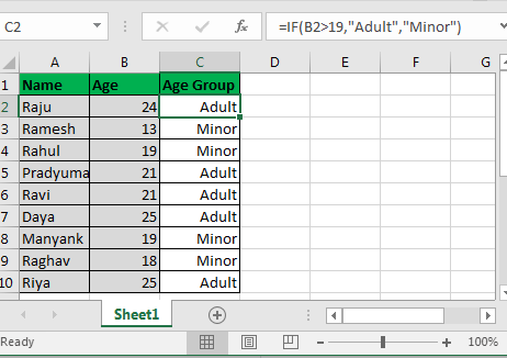
Syntax:
=IF(condition, value if TRUE, value if FALSE)
The IF statement in Excel checks the condition and returns the specified value if the condition is TRUE and another specified value if FALSE. At the place of value if TRUE and value of FALSE, you can put a value, a text within quotes, another formula or even another if statement (nested IF statement, we will talk about it).
Pro Note: IF in Excel 2016, 2013, and 2010 can have up to 64 nested IF statements. In Excel 2007 it was only 7.
The best thing about the IF statement is that you can customise TRUE and FALSE results. And this is what it is used for. Let’s see how…
IF Example 1:
Assume you have a list of people. Now you want to know how many of them are adults and how many are minors.
Let’s say people whose age is greater than 19 are Adults and who are less than 19 are minor.
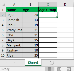
In Cell C2 write this excel IF statement and drag it down:
=IF(B2>19,»Adult»,»Minor»)
Here, Excel will simply check if the value in cell B2 is greater than 19 or not. Since it is greater than 19, it shows Adult in C2. And it does the same for all cells. Finally, we get this:

This was a simple example of an IF function in Excel. However, most of the time you would require nested IF or a combination of IF with other Excel functions.
Let’s have another example of the IF statement.
Example 2. Nested IF in Excel To Check Multiple Conditions
Assume, in a given list, you are required to tell if a kid is an Adult or “Teenager or KID”. And if Minor is then he is a teenager (between the age of 13 and 19) or a kid (below the age of 13).
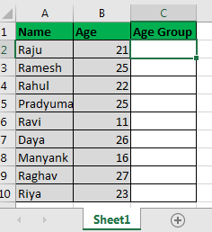
So here we have to do this
IF (is student’s age <20, if yes checkif(is student’s age <13, if yes then show “Kid”, If no then show “Teenager”), if No then show “Adult”)
There are other ways to do it but for the sake of understanding, we are taking this example.
Info: Most formulas are solved inside out but not IF statements.
In a nested IF function, outer IF is solved first and then the inner IF.
this is a basic diagram of the nested IFs control flow.
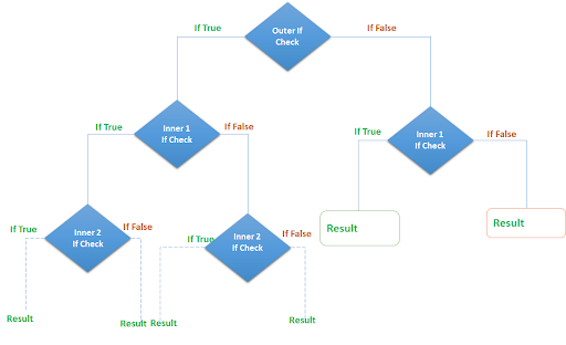
In cell C2, write this IF formula and drag it down to cell C10:
=IF(B6<20,IF(B6<13,»KID»,»Teenager»),»Adult»)
This is the final product we will have.
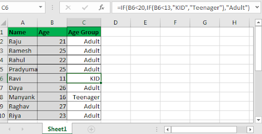
Now, let’s understand this. It’s easy.
IF(B6<20: this statement checks if the value in B6 is less than 20 not.
Since it is not, it skips the Value IF TRUE (IF(B6<13,»KID»,»Teenager»)) part and jumps to Value IF FALSE part and shows “Adult”.
Since most of them are above or equal to the age of 20, they are shown as “Adult”.
Note that Ravi is shown as “KID” as his age is 11 and Manyank is shown as “Teenager” as his age 16.
First, excel checks if Ravi’s age is <20. It’s TRUE. The control then moves to a TRUE section that contains another IF statement IF(B6<13. Next
Excel checks if Ravi<13. It’s TRUE. Control moves to the TRUE section of the IF. It contains “KID” and therefore it shows “KID” there.
Important Notes:
- Nested IFs are solved inwards. The outer IF acts as a gateway to inner IF.
- In Excel 2016, 2013 and 2010, you can have up to 64 steps of IF statements. In earlier Excel versions, it was only 7.
- IF supports logical these operators = (equals to),< (less than), > (greater than) ,<= (less than or equal to),>= (greater than or equal to, <> (not equal to)
- FALSE statements are optional, but TRUE options are mandatory.
Related Articles:
IF function with Wildcards
IF with OR Function in Excel
IF with AND Function in Excel
Popular Articles:
50 Excel Shortcut to Increase Your Productivity
How to use the VLOOKUP Function in Excel
How to use the COUNTIF function in Excel 2016
How to Use SUMIF Function in Excel
Excel IF Function – Introduction
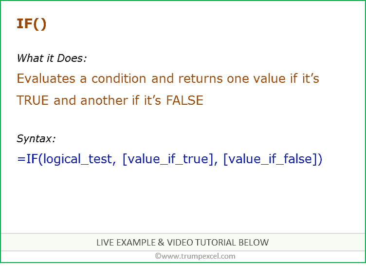
When to use Excel IF Function
IF function in Excel is best suited for situations where you check whether a condition is TRUE or FALSE. If it’s TRUE, the function returns a specified value/reference, and if not then it returns another specified value/reference.
What it Returns
It returns whatever value you specify for the TRUE or FALSE condition.
Syntax
=IF(logical_test, [value_if_true], [value_if_false])
Input Arguments
- logical_test – this is the condition that you want to test. It could be a logical expression that can evaluate to TRUE or FALSE. This can either be a cell reference, a result of some other formula, or can be manually entered.
- [value_if_true] – (Optional) This is the value that is returned when the logical_test evaluates to TRUE.
- [value_if_false] – (Optional) This is the value that is returned when the logical_test evaluates to FALSE.
Important Notes About using IF Function in Excel
- A maximum of 64 nested IF conditions can be tested in the formula.
- If any of the argument is an array, each element of the array is evaluated.
- If you omit the FALSE argument (value_if_false), i.e., there is only a comma after the value_if_true argument, the function would return a 0 when the condition is FALSE.
- For example, in the example below, the formula is =IF(A1>20,”Approve”,), where the value_if_false is not specified, however, the value_if_true argument is still followed by a comma. This would return 0 whenever the checked condition is not met.

- For example, in the example below, the formula is =IF(A1>20,”Approve”,), where the value_if_false is not specified, however, the value_if_true argument is still followed by a comma. This would return 0 whenever the checked condition is not met.
- If you omit the TRUE argument (value_if_true), and specify only the value_if_false argument, the function would return a 0 when the condition is TRUE.
- For example, in the example below, the formula is =IF(A1>20,,”Approve”), where the value_if_true is not specified (only a comma is used to then specify the value_if_false value). This would return 0 whenever the checked condition is met.

- For example, in the example below, the formula is =IF(A1>20,,”Approve”), where the value_if_true is not specified (only a comma is used to then specify the value_if_false value). This would return 0 whenever the checked condition is met.
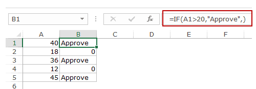

Excel IF Function – Examples
Here are five practical examples of using the IF function in Excel.
Example 1: Using Excel IF function to Check a Simple Numeric Condition
When using Excel IF function with numbers, you can use a variety of operators to check a condition. Here is a list of operators you can use:

Below is a simple example where students marks are checked. If the marks are more than or equal to 35, the function returns Pass, else it returns Fail.
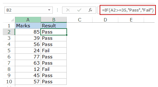
Example 2: Using Nested IF to Check a Sequence of Conditions
Excel IF Function can take up to 64 conditions at once. While it’s inadvisable to create long Nested IF functions, in the case of limited conditions, you can create a formula that checks conditions in a sequence.
In the example below, we check for two conditions.
- The first condition checks whether the marks are less than 35. If this is TRUE it returns Fail.
- In case the first condition is FALSE, which means that the student scored above or equal to 35, it checks for another condition. It checks if the marks are greater than or equal to 75. If this is true, it returns Distinction, else it simply returns Pass.
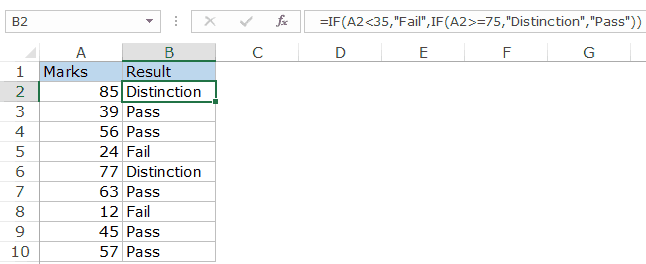
Example 3: Calculating Commissions Using Excel IF Function
Excel If Function allows you to perform calculations in the value section. A good example of this is calculating the sales commission for sales rep using the IF function.
In the example below, a sales rep gets no commission if the sales are less than 50K, gets a 2% commission if the sales are between 50-100K and 4% commission if the sales are more than 100K.
Here is the formula used:
=IF(B2<50,0,If(B2<100,B2*2%,B2*4%))
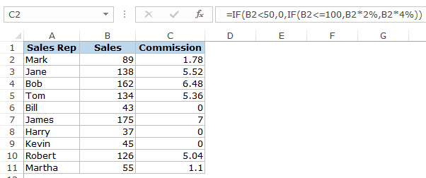
In the formula used in the example above, the calculation is done within the IF function itself. When the sales value is between 50-100K, it returns B2*2%, which is the 2% commission based on the sales value.
Example 4: Using Logical Operators (AND/OR) in Excel IF Function
You can use logical operators (AND/OR) within the IF function to test multiple conditions at once.
For example, suppose you’ve to select students for the scholarship based on marks and attendance. In the example shown below, a student is eligible only if he scores more than 80 and has the attendance of more than 80%.

You can use the AND function within the IF function to first check whether both these conditions are met or not. If the conditions are met, the function returns Eligible, else it returns Not Eligible.
Here is the formula that will do this:
=IF(AND(B2>80,C2>80%),”Yes”,”No”)
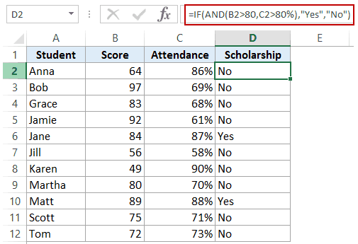
Example 5: Converting all Errors to Zero using Excel IF function
Excel IF function can also be used to get rid of cells that contain errors. You can convert the error values to blanks or zeros or any other value.
Here is the formula that will do it:
=IF(ISERROR(A1),0,A1)
The formula returns a 0 when there is an error value, else it returns the value in the cell.
NOTE: If you’re using Excel 2007 or versions after it, you can also use the IFERROR function to do this.
Similarly, you can also handle blank cells. In case of blank cells, use the ISBLANK function as shown below:
=IF(ISBLANK(A1),0,A1)

Excel IF Function – Video Tutorial
Related Excel Functions:
- Excel AND Function.
- Excel OR Function.
- Excel NOT Function.
- Excel IFS Function.
- Excel IFERROR Function.
- Excel FALSE Function.
- Excel TRUE Function
Other Excel tutorials you may find useful:
- Avoid Nested IF Function in Excel by using VLOOKUP