
Содержание
- Using IF with AND, OR and NOT functions
- Examples
- Using AND, OR and NOT with Conditional Formatting
- Need more help?
- See also
- IF Excel Function
- What is IF Function in Excel?
- Syntax of the IF Excel Function
- How to Use IF Function in Excel?
- Example #1
- Example #2
- Example #3
- Example #4
- Example #5
- Guidelines for the Multiple IF Statements
- Frequently Asked Question
- IF Excel Function Video
- Recommended Articles
Using IF with AND, OR and NOT functions
The IF function allows you to make a logical comparison between a value and what you expect by testing for a condition and returning a result if that condition is True or False.
=IF(Something is True, then do something, otherwise do something else)
But what if you need to test multiple conditions, where let’s say all conditions need to be True or False ( AND), or only one condition needs to be True or False ( OR), or if you want to check if a condition does NOT meet your criteria? All 3 functions can be used on their own, but it’s much more common to see them paired with IF functions.
Use the IF function along with AND, OR and NOT to perform multiple evaluations if conditions are True or False.
IF(AND()) — IF(AND(logical1, [logical2], . ), value_if_true, [value_if_false]))
IF(OR()) — IF(OR(logical1, [logical2], . ), value_if_true, [value_if_false]))
IF(NOT()) — IF(NOT(logical1), value_if_true, [value_if_false]))
The condition you want to test.
The value that you want returned if the result of logical_test is TRUE.
The value that you want returned if the result of logical_test is FALSE.
Here are overviews of how to structure AND, OR and NOT functions individually. When you combine each one of them with an IF statement, they read like this:
AND – =IF(AND(Something is True, Something else is True), Value if True, Value if False)
OR – =IF(OR(Something is True, Something else is True), Value if True, Value if False)
NOT – =IF(NOT(Something is True), Value if True, Value if False)
Examples
Following are examples of some common nested IF(AND()), IF(OR()) and IF(NOT()) statements. The AND and OR functions can support up to 255 individual conditions, but it’s not good practice to use more than a few because complex, nested formulas can get very difficult to build, test and maintain. The NOT function only takes one condition.

Here are the formulas spelled out according to their logic:
=IF(AND(A2>0,B2 0,B4 50),TRUE,FALSE)
IF A6 (25) is NOT greater than 50, then return TRUE, otherwise return FALSE. In this case 25 is not greater than 50, so the formula returns TRUE.
IF A7 (“Blue”) is NOT equal to “Red”, then return TRUE, otherwise return FALSE.
Note that all of the examples have a closing parenthesis after their respective conditions are entered. The remaining True/False arguments are then left as part of the outer IF statement. You can also substitute Text or Numeric values for the TRUE/FALSE values to be returned in the examples.
Here are some examples of using AND, OR and NOT to evaluate dates.

Here are the formulas spelled out according to their logic:
IF A2 is greater than B2, return TRUE, otherwise return FALSE. 03/12/14 is greater than 01/01/14, so the formula returns TRUE.
=IF(AND(A3>B2,A3 B2,A4 B2),TRUE,FALSE)
IF A5 is not greater than B2, then return TRUE, otherwise return FALSE. In this case, A5 is greater than B2, so the formula returns FALSE.

Using AND, OR and NOT with Conditional Formatting
You can also use AND, OR and NOT to set Conditional Formatting criteria with the formula option. When you do this you can omit the IF function and use AND, OR and NOT on their own.
From the Home tab, click Conditional Formatting > New Rule. Next, select the “ Use a formula to determine which cells to format” option, enter your formula and apply the format of your choice.
 Edit Rule dialog showing the Formula method» loading=»lazy»>
Using the earlier Dates example, here is what the formulas would be.

If A2 is greater than B2, format the cell, otherwise do nothing.
=AND(A3>B2,A3 B2,A4 B2)
If A5 is NOT greater than B2, format the cell, otherwise do nothing. In this case A5 is greater than B2, so the result will return FALSE. If you were to change the formula to =NOT(B2>A5) it would return TRUE and the cell would be formatted.
Note: A common error is to enter your formula into Conditional Formatting without the equals sign (=). If you do this you’ll see that the Conditional Formatting dialog will add the equals sign and quotes to the formula — =»OR(A4>B2,A4
Need more help?

See also
You can always ask an expert in the Excel Tech Community or get support in the Answers community.
Источник
IF Excel Function


What is IF Function in Excel?
IF function in Excel evaluates whether a given condition is met and returns a value depending on whether the result is “true” or “false”. It is a conditional function of Excel, which returns the result based on the fulfillment or non-fulfillment of the given criteria.
For example, the IF formula in Excel can be applied as follows:
“=IF(condition A,“value B”,“value C”)”
The IF excel function returns “value B” if condition A is met and returns “value C” if condition A is not met.
It is often used to make logical interpretations which help in decision-making.
Table of contents
Syntax of the IF Excel Function
The syntax of the IF function is shown in the following image:

The IF excel function accepts the following arguments:
- Logical_test: It refers to the condition to be evaluated. The condition can be a value or a logical expression.
- Value_if_true: It is the value returned as a result when the condition is “true”.
- Value_if_false: It is the value returned as a result when the condition is “false”.
In the formula, the “logical_test” is a required argument, whereas the “value_if_true” and “value_if_false” are optional arguments.
| Operator | Meaning |
|---|---|
| = | Equal to |
| > | Greater than |
| >= | Greater than or equal to |
| Not equal to |
How to Use IF Function in Excel?
Let us understand the working of the IF function with the help of the following examples in Excel.
Example #1
If there is no oxygen on a planet, life is impossible. If oxygen is available on a planet, then life is possible. The following table shows a list of planets in column A and the information on the availability of oxygen in column B. We have to find the planets where life is possible, based on the condition of oxygen availability.

Let us apply the IF formula to cell C2 to find out whether life is possible on the planets listed in the table.
The IF formula is stated as follows:
“=IF(B2=“Yes”, “Life is Possible”, “Life is Not Possible”)
The succeeding image shows the IF formula applied to cell C2.

The subsequent image shows how the IF formula is applied to the range of cells C2:C5.

Drag the cells to view the output of all the planets.

The output in the below worksheet shows life is possible on the planet Earth.
Flow Chart of Generic IF Excel Function

The IF Function Flow Chart for Mars (Example #1)

The flow of IF function flowchart for Jupiter and Venus is the same as the IF function flowchart for Mars (Example #1).
The IF Function Flow Chart for Earth

Hence, the IF excel function allows making logical comparisons between values. The modus operandi of the IF function is stated as: If something is true, then do something; otherwise, do something else.
Example #2
The following table shows a list of years. We want to find out if the given year is a leap year or not.
A leap year has 366 days; the extra day is the 29th of February. The criteria for a leap year are stated as follows:
- The year will be exactly divisible by 4 and not exactly be divisible by 100 or
- The year will be exactly divisible by 400.

In this example, we will use the IF function along with the AND, OR, and MOD functions to find the leap years.
We use the MOD function to find a remainder after a dividend is divided by a divisor.
We will apply the MOD function to the conditions as follows:
If MOD(year,4)=0 and MOD(year,100)<>(is not equal to) 0, then the year is a leap year.
If MOD(year,400)=0, then the year is a leap year; otherwise, the year is not a leap year.
The IF formula is stated as follows:
“=IF(OR(AND((MOD(year,4)=0),(MOD(year,100)<>0)),(MOD(year,400)=0)),“Leap Year”, “Not A Leap Year”)”
The argument “year” refers to a reference value.
The following images show the output of the IF formula applied in the range of cells.


The following image shows how the IF formula is applied to the range of cells B2:B18.

The succeeding table shows the years 1960, 2028, and 2148 as leap years and the remaining as non-leap years.

The result of the IF excel formula is displayed for the range of cells B2:B18 in the following image.

Example #3
The succeeding table shows a list of drivers and the directions they undertook to reach the destination. It is preceded by an image of the road intersection explaining the turns taken by the drivers and their destinations. The right turn leads to town B, and the left turn leads to town C. Identify the driver’s destination to town B and town C.
Road Intersection Image


Let us apply the IF excel function to find the destination. Here, the condition is mentioned as follows:
- If the driver turns right, he/she reaches town B.
- If the driver turns left, he/she reaches town C.
We use the following IF formula to find the destination:
“=IF(B2=“Left”, “Town C”, “Town B”)”
The succeeding image shows the output of the IF formula applied to cell C2.

Drag the cells to use the formula in the range C2:C11. Finally, we get the destinations of each driver for their turning movements.
The below image displays the IF formula applied to the range.

The output of the IF formula and the destinations are displayed in the succeeding image.

The result shows that six drivers reached town C, and the remaining four have reached town B.
Example #4
The following table shows a list of items and their inventory levels. We want to check if the specific item is available in the inventory or not using the IF function.

Let us list the name of items in column A and the number of items in column B. The list of data to be validated for the entire items list is shown in the cell E2 of the below image.

The VLOOKUP function looks up the values referring to the number of items, and the IF function will check whether the item number is greater than zero or not.
We will apply the following IF formula in the F2 cell:
“=IF(VLOOKUP(E2,A2:B11,2,0)=0, “Item Not Available”,“Item Available”)”
If the lookup value of an item is equal to 0, then the item is not available; else, the item is available.
The succeeding image shows the result of the IF formula in the cell F2.

Select “bat” in the E2 item cell to know whether the item is available or not in the inventory (as shown in the following image).

Example #5
The following table shows the list of students and their marks. The grade criteria are provided based on the marks obtained by the students. We want to find the grade of each student in the list.

We apply the Nested IF in Excel since we have multiple criteria to find and decide each student’s grade.
The Nesting of IF function uses the IF function inside another IF formula when multiple conditions are to be fulfilled.
The syntax of Nesting of IF function is stated as follows:
“=IF( condition1, value_if_true1, IF( condition2, value_if_true2, value_if_false2 ))”
The succeeding table represents the range of scores and the grades, respectively.

Let us apply the multiple IF conditions with AND function in the below-nested formula to find out the grade of the students:
“=IF((B2>=95),“A”,IF(AND(B2>=85,B2 =75,B2 =61,B2 =95
If the formula returns,
- Value_if_true, execute: “A” (Grade A) else(comma) enter value_if_false
- Value_if_false, then the formula finds another IF condition and enter IF condition
Second Logical Test: B2>=85(logical expression 1) and B2 =75(logical expression 1) and B2 =61(logical expression 1) and B2 
The succeeding image shows the IF nested formula applied to the range.

The grades of the students are listed in the following table.

Guidelines for the Multiple IF Statements
The guidelines for the multiple IF statements are listed as follows:
- Use nested IF function to a limited extent as multiple IF statements require a great deal of thought to be accurate.
- Multiple IF statementsMultiple IF StatementsIn Excel, multiple IF conditions are IF statements that are contained within another IF statement. They are used to test multiple conditions at the same time and return distinct values. Additional IF statements can be included in the ‘value if true’ and ‘value if false’ arguments of a standard IF formula.read more require multiple parentheses (), which is often difficult to manage. Excel provides a way to check the color of each opening and closing parenthesis to avoid this situation. The last closing parenthesis color will always be black, denoting the end of the formula statement.
- Whenever we pass a string value for the arguments “value_if_true” and “value_if_false” or test a reference against a string value, enclose the string value in double quotes. Passing a string value without quotes will result in “#NAME?” error.
Frequently Asked Question
The Excel IF function is a logical function that checks the given criteria and returns one value for a “true” and another value for a “false” result.
The syntax of the IF function is stated as follows:
“=IF(logical_test, [value_if_true], [value_if_false])”
The arguments are as follows:
1. Logical_test – It refers to a value or condition that is tested.
2. Value_if_true – It is the value returned when the condition logical_test is “true.”
3. Value_if_false – It is the value returned when the condition logical_test is “false.”
The “logical_test” is a required argument, whereas the “value_if_true” and “value_if_false” are optional arguments.
The IF Excel statement for multiple conditions is created by using multiple IF functions in a single formula.
The syntax of IF function with multiple conditions is stated as follows:
“=IF (condition 1_“true”, do something, IF (condition 2_“true”, do something, IF (condition 3_ “true”, do something, else do something)))”
On checking a formula, if it finds an error, it returns another value specified by the user. Else it returns the result of the formula.
The syntax is stated as follows:
“=IFERROR(value, value_if_error)”
Where,
• Value – It refers to the value to be tested.
• Value_if_error – It refers to the value to be returned if the formula returns an error.
Both the arguments are the required arguments.
IF Excel Function Video
Recommended Articles
This has been a guide to the IF function in Excel. Here we discuss how to use the IF function along with examples and downloadable templates. You may also look at these useful functions –
Источник
IF function
The IF function is one of the most popular functions in Excel, and it allows you to make logical comparisons between a value and what you expect.
So an IF statement can have two results. The first result is if your comparison is True, the second if your comparison is False.
For example, =IF(C2=”Yes”,1,2) says IF(C2 = Yes, then return a 1, otherwise return a 2).

Use the IF function, one of the logical functions, to return one value if a condition is true and another value if it’s false.
IF(logical_test, value_if_true, [value_if_false])
For example:
-
=IF(A2>B2,»Over Budget»,»OK»)
-
=IF(A2=B2,B4-A4,»»)
|
Argument name |
Description |
|---|---|
|
logical_test (required) |
The condition you want to test. |
|
value_if_true (required) |
The value that you want returned if the result of logical_test is TRUE. |
|
value_if_false (optional) |
The value that you want returned if the result of logical_test is FALSE. |
Simple IF examples

-
=IF(C2=”Yes”,1,2)
In the above example, cell D2 says: IF(C2 = Yes, then return a 1, otherwise return a 2)

-
=IF(C2=1,”Yes”,”No”)
In this example, the formula in cell D2 says: IF(C2 = 1, then return Yes, otherwise return No)As you see, the IF function can be used to evaluate both text and values. It can also be used to evaluate errors. You are not limited to only checking if one thing is equal to another and returning a single result, you can also use mathematical operators and perform additional calculations depending on your criteria. You can also nest multiple IF functions together in order to perform multiple comparisons.

-
=IF(C2>B2,”Over Budget”,”Within Budget”)
In the above example, the IF function in D2 is saying IF(C2 Is Greater Than B2, then return “Over Budget”, otherwise return “Within Budget”)

-
=IF(C2>B2,C2-B2,0)
In the above illustration, instead of returning a text result, we are going to return a mathematical calculation. So the formula in E2 is saying IF(Actual is Greater than Budgeted, then Subtract the Budgeted amount from the Actual amount, otherwise return nothing).

-
=IF(E7=”Yes”,F5*0.0825,0)
In this example, the formula in F7 is saying IF(E7 = “Yes”, then calculate the Total Amount in F5 * 8.25%, otherwise no Sales Tax is due so return 0)
Note: If you are going to use text in formulas, you need to wrap the text in quotes (e.g. “Text”). The only exception to that is using TRUE or FALSE, which Excel automatically understands.
Common problems
|
Problem |
What went wrong |
|---|---|
|
0 (zero) in cell |
There was no argument for either value_if_true or value_if_False arguments. To see the right value returned, add argument text to the two arguments, or add TRUE or FALSE to the argument. |
|
#NAME? in cell |
This usually means that the formula is misspelled. |
Need more help?
You can always ask an expert in the Excel Tech Community or get support in the Answers community.
See Also
IF function — nested formulas and avoiding pitfalls
IFS function
Using IF with AND, OR and NOT functions
COUNTIF function
How to avoid broken formulas
Overview of formulas in Excel
Need more help?
The IF function runs a logical test and returns one value for a TRUE result, and another value for a FALSE result. The result from IF can be a value, a cell reference, or even another formula. By combining the IF function with other logical functions like AND and OR, you can test more than one condition at a time.
Syntax
The generic syntax for the IF function looks like this:
=IF(logical_test,[value_if_true],[value_if_false])The first argument, logical_test, is typically an expression that returns either TRUE or FALSE. The second argument, value_if_true, is the value to return when logical_test is TRUE. The last argument, value_if_false, is the value to return when logical_test is FALSE. Both value_if_true and value_if_false are optional, but you must provide one or the other. For example, if cell A1 contains 80, then:
=IF(A1>75,TRUE) // returns TRUE
=IF(A1>75,"OK") // returns "OK"
=IF(A1>85,"OK") // returns FALSE
=IF(A1>75,10,0) // returns 10
=IF(A1>85,10,0) // returns 0
=IF(A1>75,"Yes","No") // returns "Yes"
=IF(A1>85,"Yes","No") // returns "No"
Notice that text values like «OK», «Yes», «No», etc. must be enclosed in double quotes («»). However, numeric values should not be enclosed in quotes.
Logical tests
The IF function supports logical operators (>,<,<>,=) when creating logical tests. Most commonly, the logical_test in IF is a complete logical expression that will evaluate to TRUE or FALSE. The table below shows some common examples:
| Goal | Logical test |
|---|---|
| If A1 is greater than 75 | A1>75 |
| If A1 equals 100 | A1=100 |
| If A1 is less than or equal to 100 | A1<=100 |
| If A1 equals «Red» | A1=»red» |
| If A1 is not equal to «Red» | A1<>»red» |
| If A1 is less than B1 | A1<B1 |
| If A1 is empty | A1=»» |
| If A1 is not empty | A1<>»» |
| If A1 is less than current date | A1<TODAY() |
Notice text values must be enclosed in double quotes («»), but numbers do not. The IF function does not support wildcards, but you can combine IF with COUNTIF to get basic wildcard functionality. To test for substrings in a cell, you can use the IF function with the SEARCH function.
Pass or Fail example
In the worksheet shown above, we want to assign either «Pass» or «Fail» based on a test score. A passing score is 70 or higher. The formula in D6, copied down, is:
=IF(C5>=70,"Pass","Fail")
Translation: If the value in C5 is greater than or equal to 70, return «Pass». Otherwise, return «Fail».
Note that the logical flow of this formula can be reversed. This formula returns the same result:
=IF(C5<70,"Fail","Pass")
Translation: If the value in C5 is less than 70, return «Fail». Otherwise, return «Pass».
Both formulas above, when copied down, will return correct results.
Note: If you are new to the idea of formula criteria, this article explains many examples.
Assign points based on color
In the worksheet below, we want to assign points based on the color in column B. If the color is «red», the result should be 100. If the color is «blue», the result should be 125. This requires that we use a formula based on two IF functions, one nested inside the other. The formula in C5, copied down, is:
=IF(B5="red",100,IF(B5="blue",125))
Translation: IF the value in B5 is «red», return 100. Else, if the value in B5 is «blue», return 125.

There are three things to notice in this example:
- The formula will return FALSE if the value in B5 is anything except «red» or «blue»
- The text values «red» and «blue» must be enclosed in double quotes («»)
- The IF function is not case-sensitive and will match «red», «Red», «RED», or «rEd».
This is a simple example of a nested IFs formula. See below for a more complex example.
Return another formula
The IF function can return another formula as a result. For example, the formula below will return A1*5% when A1 is less than 100, and A1*7% when A1 is greater than or equal to 100:
=IF(A1<100,A1*5%,A1*7%)
Nested IF statements
The IF function can be «nested». A «nested IF» refers to a formula where at least one IF function is nested inside another in order to test for more conditions and return more possible results. Each IF statement needs to be carefully «nested» inside another so that the logic is correct. For example, the following formula can be used to assign a grade rather than a pass / fail result:
=IF(C6<70,"F",IF(C6<75,"D",IF(C6<85,"C",IF(C6<95,"B","A"))))
Up to 64 IF functions can be nested. However, in general, you should consider other functions, like VLOOKUP or XLOOKUP for more complex scenarios, because they can handle more conditions in a more streamlined fashion. For a more details see this article on nested IFs.
Note: the newer IFS function is designed to handle multiple conditions without nesting. However, a lookup function like VLOOKUP or XLOOKUP is usually a better approach unless the logic for each condition is custom.
IF with AND, OR, NOT
The IF function can be combined with the AND function and the OR function. For example, to return «OK» when A1 is between 7 and 10, you can use a formula like this:
=IF(AND(A1>7,A1<10),"OK","")
Translation: if A1 is greater than 7 and less than 10, return «OK». Otherwise, return nothing («»).
To return B1+10 when A1 is «red» or «blue» you can use the OR function like this:
=IF(OR(A1="red",A1="blue"),B1+10,B1)
Translation: if A1 is red or blue, return B1+10, otherwise return B1.
=IF(NOT(A1="red"),B1+10,B1)
Translation: if A1 is NOT red, return B1+10, otherwise return B1.
IF cell contains specific text
Because the IF function does not support wildcards, it is not obvious how to configure IF to check for a specific substring in a cell. A common approach is to combine the ISNUMBER function and the SEARCH function to create a logical test like this:
=ISNUMBER(SEARCH(substring,A1)) // returns TRUE or FALSEFor example, to check for the substring «xyz» in cell A1, you can use a formula like this:
=IF(ISNUMBER(SEARCH("xyz",A1)),"Yes","No")Read a detailed explanation here.
More information
- Read more about nested IFs
- Learn how to use VLOOKUP instead of nested IFs (video)
- 50 Examples of formula criteria
Notes
- The IF function is not case-sensitive.
- To count values conditionally, use the COUNTIF or the COUNTIFS functions.
- To sum values conditionally, use the SUMIF or the SUMIFS functions.
- If any of the arguments to IF are supplied as arrays, the IF function will evaluate every element of the array.
What is IF Function in Excel?
IF function in Excel evaluates whether a given condition is met and returns a value depending on whether the result is “true” or “false”. It is a conditional function of Excel, which returns the result based on the fulfillment or non-fulfillment of the given criteria.
For example, the IF formula in Excel can be applied as follows:
“=IF(condition A,“value B”,“value C”)”
The IF excel function returns “value B” if condition A is met and returns “value C” if condition A is not met.
It is often used to make logical interpretations which help in decision-making.
Table of contents
- What is IF Function in Excel?
- Syntax of the IF Excel Function
- How to Use IF Function in Excel?
- Example #1
- Example #2
- Example #3
- Example #4
- Example #5
- Guidelines for the Multiple IF Statements
- Frequently Asked Question
- IF Excel Function Video
- Recommended Articles
Syntax of the IF Excel Function
The syntax of the IF function is shown in the following image:
The IF excel function accepts the following arguments:
- Logical_test: It refers to the condition to be evaluated. The condition can be a value or a logical expression.
- Value_if_true: It is the value returned as a result when the condition is “true”.
- Value_if_false: It is the value returned as a result when the condition is “false”.
In the formula, the “logical_test” is a required argument, whereas the “value_if_true” and “value_if_false” are optional arguments.
The IF formula uses logical operators to evaluate the values in a range of cells. The following table shows the different logical operatorsLogical operators in excel are also known as the comparison operators and they are used to compare two or more values, the return output given by these operators are either true or false, we get true value when the conditions match the criteria and false as a result when the conditions do not match the criteria.read more and their meaning.
| Operator | Meaning |
|---|---|
| = | Equal to |
| > | Greater than |
| >= | Greater than or equal to |
| < | Less than |
| <= | Less than or equal to |
| <> | Not equal to |
How to Use IF Function in Excel?
Let us understand the working of the IF function with the help of the following examples in Excel.
You can download this IF Function Excel Template here – IF Function Excel Template
Example #1
If there is no oxygen on a planet, life is impossible. If oxygen is available on a planet, then life is possible. The following table shows a list of planets in column A and the information on the availability of oxygen in column B. We have to find the planets where life is possible, based on the condition of oxygen availability.
Let us apply the IF formula to cell C2 to find out whether life is possible on the planets listed in the table.
The IF formula is stated as follows:
“=IF(B2=“Yes”, “Life is Possible”, “Life is Not Possible”)
The succeeding image shows the IF formula applied to cell C2.
The subsequent image shows how the IF formula is applied to the range of cells C2:C5.
Drag the cells to view the output of all the planets.
The output in the below worksheet shows life is possible on the planet Earth.
Flow Chart of Generic IF Excel Function
The IF Function Flow Chart for Mars (Example #1)
The flow of IF function flowchart for Jupiter and Venus is the same as the IF function flowchart for Mars (Example #1).
The IF Function Flow Chart for Earth
Hence, the IF excel function allows making logical comparisons between values. The modus operandi of the IF function is stated as: If something is true, then do something; otherwise, do something else.
Example #2
The following table shows a list of years. We want to find out if the given year is a leap year or not.
A leap year has 366 days; the extra day is the 29th of February. The criteria for a leap year are stated as follows:
- The year will be exactly divisible by 4 and not exactly be divisible by 100 or
- The year will be exactly divisible by 400.
In this example, we will use the IF function along with the AND, OR, and MOD functions to find the leap years.
We use the MOD function to find a remainder after a dividend is divided by a divisor.
The AND functionThe AND function in Excel is classified as a logical function; it returns TRUE if the specified conditions are met, otherwise it returns FALSE.read more evaluates both the conditions of the leap years for the value “true”. The OR functionThe OR function in Excel is used to test various conditions, allowing you to compare two values or statements in Excel. If at least one of the arguments or conditions evaluates to TRUE, it will return TRUE. Similarly, if all of the arguments or conditions are FALSE, it will return FASLE.read more evaluates either of the condition for the value “true”.
We will apply the MOD function to the conditions as follows:
If MOD(year,4)=0 and MOD(year,100)<>(is not equal to) 0, then the year is a leap year.
or
If MOD(year,400)=0, then the year is a leap year; otherwise, the year is not a leap year.
The IF formula is stated as follows:
“=IF(OR(AND((MOD(year,4)=0),(MOD(year,100)<>0)),(MOD(year,400)=0)),“Leap Year”, “Not A Leap Year”)”
The argument “year” refers to a reference value.
The following images show the output of the IF formula applied in the range of cells.
The following image shows how the IF formula is applied to the range of cells B2:B18.
The succeeding table shows the years 1960, 2028, and 2148 as leap years and the remaining as non-leap years.
The result of the IF excel formula is displayed for the range of cells B2:B18 in the following image.
Example #3
The succeeding table shows a list of drivers and the directions they undertook to reach the destination. It is preceded by an image of the road intersection explaining the turns taken by the drivers and their destinations. The right turn leads to town B, and the left turn leads to town C. Identify the driver’s destination to town B and town C.
Road Intersection Image
Let us apply the IF excel function to find the destination. Here, the condition is mentioned as follows:
- If the driver turns right, he/she reaches town B.
- If the driver turns left, he/she reaches town C.
We use the following IF formula to find the destination:
“=IF(B2=“Left”, “Town C”, “Town B”)”
The succeeding image shows the output of the IF formula applied to cell C2.
Drag the cells to use the formula in the range C2:C11. Finally, we get the destinations of each driver for their turning movements.
The below image displays the IF formula applied to the range.
The output of the IF formula and the destinations are displayed in the succeeding image.
The result shows that six drivers reached town C, and the remaining four have reached town B.
Example #4
The following table shows a list of items and their inventory levels. We want to check if the specific item is available in the inventory or not using the IF function.
Let us list the name of items in column A and the number of items in column B. The list of data to be validated for the entire items list is shown in the cell E2 of the below image.
We use the Excel IF along with the VLOOKUP functionThe VLOOKUP excel function searches for a particular value and returns a corresponding match based on a unique identifier. A unique identifier is uniquely associated with all the records of the database. For instance, employee ID, student roll number, customer contact number, seller email address, etc., are unique identifiers.
read more to check the availability of the items in the inventory.
The VLOOKUP function looks up the values referring to the number of items, and the IF function will check whether the item number is greater than zero or not.
We will apply the following IF formula in the F2 cell:
“=IF(VLOOKUP(E2,A2:B11,2,0)=0, “Item Not Available”,“Item Available”)”
If the lookup value of an item is equal to 0, then the item is not available; else, the item is available.
The succeeding image shows the result of the IF formula in the cell F2.
Select “bat” in the E2 item cell to know whether the item is available or not in the inventory (as shown in the following image).
Example #5
The following table shows the list of students and their marks. The grade criteria are provided based on the marks obtained by the students. We want to find the grade of each student in the list.
We apply the Nested IF in Excel since we have multiple criteria to find and decide each student’s grade.
The Nesting of IF function uses the IF function inside another IF formula when multiple conditions are to be fulfilled.
The syntax of Nesting of IF function is stated as follows:
“=IF( condition1, value_if_true1, IF( condition2, value_if_true2, value_if_false2 ))”
The succeeding table represents the range of scores and the grades, respectively.
Let us apply the multiple IF conditions with AND function in the below-nested formula to find out the grade of the students:
“=IF((B2>=95),“A”,IF(AND(B2>=85,B2<=94),“B”,IF(AND(B2>=75,B2<=84),“C”,IF(AND(B2>=61,B2<=74),“D”,“F”))))”
The IF function checks the logical condition as shown in the formula below:
“=IF(logical_test, [value_if_true],[value_if_false])”
We will split the above-mentioned nested formula and check the IF statements as shown below:
First Logical Test: B2>=95
If the formula returns,
- Value_if_true, execute: “A” (Grade A) else(comma) enter value_if_false
- Value_if_false, then the formula finds another IF condition and enter IF condition
Second Logical Test: B2>=85(logical expression 1) and B2<=94(logical expression 2)
(We use AND function to check the multiple logical expressions as the two given conditions are to be evaluated for “true.”)
If the formula returns,
- Value_if_true, execute: “B” (Grade B) else(comma) enter value_if_false
- Value_if_false, then the formula finds another IF condition and enter IF condition
Third Logical Test: B2>=75(logical expression 1) and B2<=84(logical expression 2)
(We use AND function to check the multiple logical expressions as the two given conditions are to be evaluated for “true.”)
If the formula returns,
- Value_if_true, execute: “C” (Grade C) else(comma) enter value_if_false
- value_if_false, then the formula finds another IF condition and enter IF condition
Fourth Logical Test: B2>=61(logical expression 1) and B2<=74(logical expression 2)
(We use AND function to check the multiple logical expressions as the two given conditions are to be evaluated for “true.”)
If the formula returns,
- Value_if_true, execute: “D” (Grade D) else(comma) enter value_if_false
- Value_if_false, execute: “F” (Grade F)
- Finally, close the parenthesis.
The below image displays the output of the IF formula applied to the range.
The succeeding image shows the IF nested formula applied to the range.
The grades of the students are listed in the following table.
Guidelines for the Multiple IF Statements
The guidelines for the multiple IF statements are listed as follows:
- Use nested IF function to a limited extent as multiple IF statements require a great deal of thought to be accurate.
- Multiple IF statementsIn Excel, multiple IF conditions are IF statements that are contained within another IF statement. They are used to test multiple conditions at the same time and return distinct values. Additional IF statements can be included in the ‘value if true’ and ‘value if false’ arguments of a standard IF formula.read more require multiple parentheses (), which is often difficult to manage. Excel provides a way to check the color of each opening and closing parenthesis to avoid this situation. The last closing parenthesis color will always be black, denoting the end of the formula statement.
- Whenever we pass a string value for the arguments “value_if_true” and “value_if_false” or test a reference against a string value, enclose the string value in double quotes. Passing a string value without quotes will result in “#NAME?” error.
Frequently Asked Question
1. What is the IF function in Excel?
The Excel IF function is a logical function that checks the given criteria and returns one value for a “true” and another value for a “false” result.
The syntax of the IF function is stated as follows:
“=IF(logical_test, [value_if_true], [value_if_false])”
The arguments are as follows:
1. Logical_test – It refers to a value or condition that is tested.
2. Value_if_true – It is the value returned when the condition logical_test is “true.”
3. Value_if_false – It is the value returned when the condition logical_test is “false.”
The “logical_test” is a required argument, whereas the “value_if_true” and “value_if_false” are optional arguments.
2. How to use the IF Excel function with multiple conditions?
The IF Excel statement for multiple conditions is created by using multiple IF functions in a single formula.
The syntax of IF function with multiple conditions is stated as follows:
“=IF (condition 1_“true”, do something, IF (condition 2_“true”, do something, IF (condition 3_ “true”, do something, else do something)))”
3. How to use the function IFERROR in Excel?
IF Excel Function Video
Recommended Articles
This has been a guide to the IF function in Excel. Here we discuss how to use the IF function along with examples and downloadable templates. You may also look at these useful functions –
- What is the Logical Test in Excel?A logical test in Excel results in an analytical output, either true or false. The equals to operator, “=,” is the most commonly used logical test.read more
- “Not Equal to” in Excel“Not Equal to” argument in excel is inserted with the expression <>. The two brackets posing away from each other command excel of the “Not Equal to” argument, and the user then makes excel checks if two values are not equal to each other.read more
- Data Validation ExcelThe data validation in excel helps control the kind of input entered by a user in the worksheet.read more
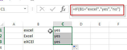
Normally, If you want to write an IF formula for text values in combining with the below two logical operators in excel, such as: “equal to” or “not equal to”.
Table of Contents
- Excel IF function check if a cell contains text(case-insensitive)
- Excel IF function check if a cell contains text (case-sensitive)
- Excel IF function check if part of cell matches specific text
- Excel IF function with Wildcards text value
- Related Formulas
- Related Functions
Excel IF function check if a cell contains text(case-insensitive)
By default, IF function is case-insensitive in excel. It means that the logical text for text values will do not recognize case in the IF formulas. For example, the following two IF formulas will get the same results when checking the text values in cells.
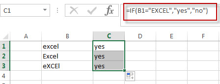
=IF(B1="excel","yes","no")
=IF(B1="EXCEl","yes","no")
The IF formula will check the values of cell B1 if it is equal to “excel” word, If it is TRUE, then return “yes”, otherwise return “no”. And the logical test in the above IF formula will check the text values in the logical_test argument, whatever the logical_test values are “Excel”, “eXcel”, or “EXCEL”, the IF formula don’t care about that if the text values is in lowercase or uppercase, It will get the same results at last.
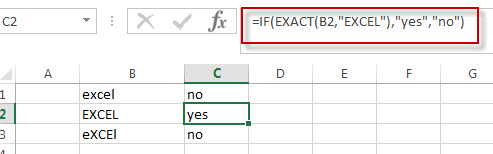
Excel IF function check if a cell contains text (case-sensitive)
If you want to check text values in cells using IF formula in excel (case-sensitive), then you need to create a case-sensitive logical test and then you can use IF function in combination with EXACT function to compare two text values. So if those two text values are exactly the same, then return TRUE. Otherwise return FALSE.
So we can write down the following IF formula combining with EXACT function:
=IF(EXACT(B1,"excel"),"yes","no")
Excel IF function check if part of cell matches specific text
If you want to check if part of text values in cell matches the specific text rather than exact match, to achieve this logic text, you can use IF function in combination with ISNUMBER and SEARCH Function in excel.
Both ISNUMBER and SEARCH functions are case-insensitive in excel.
=IF(ISNUMBER(SEARCH("x",B1)),"good","bad")
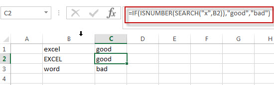
For above the IF formula, it will Check to see if B1 contain the letter x.
Also, we can use FIND function to replace the SEARCH function in the above IF formula. It will return the same results.
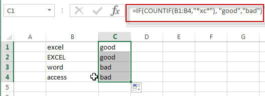
Excel IF function with Wildcards text value
If you wan to use wildcard charcter in an IF formula, for example, if any of the values in column B contains “*xc*”, then return “good”, others return “bad”. You can not directly use the wildcard characters in IF formula, and we can use IF function in combination with COUNTIF function. Let’s see the following IF formula:
=IF(COUNTIF(B1:B4,"*xc*"), "good","bad")
- Excel IF Function With Numbers
If you want to check if a cell values is between two values or checking for the range of numbers or multiple values in cells, at this time, we need to use AND or OR logical function in combination with the logical operator and IF function…
- Excel EXACT function
The Excel SEARCH function returns the number of the starting location of a substring in a text string.The syntax of the EXACT function is as below:= EXACT (text1,text2)… - Excel COUNTIF function
The Excel COUNTIF function will count the number of cells in a range that meet a given criteria.= COUNTIF (range, criteria) … - Excel ISNUMBER function
The Excel ISNUMBER function returns TRUE if the value in a cell is a numeric value, otherwise it will return FALSE. - Excel IF function
The Excel IF function perform a logical test to return one value if the condition is TRUE and return another value if the condition is FALSE…. - Excel SEARCH function
The Excel SEARCH function returns the number of the starting location of a substring in a text string.…