
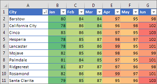
Conditional formatting can help make patterns and trends in your data more apparent. To use it, you create rules that determine the format of cells based on their values, such as the following monthly temperature data with cell colors tied to cell values.
You can apply conditional formatting to a range of cells (either a selection or a named range), an Excel table, and in Excel for Windows, even a PivotTable report.

Conditional formatting typically works the same way in a range of cells, an Excel table, or a PivotTable report. However, conditional formatting in a PivotTable report has some extra considerations:
-
There are some conditional formats that don’t work with fields in the Values area of a PivotTable report. For example, you can’t format such fields based on whether they contain unique or duplicate values. These restrictions are mentioned in the remaining sections of this article, where applicable.
-
If you change the layout of the PivotTable report by filtering, hiding levels, collapsing and expanding levels, or moving a field, the conditional format is maintained as long as the fields in the underlying data are not removed.
-
The scope of the conditional format for fields in the Values area can be based on the data hierarchy and is determined by all the visible children (the next lower level in a hierarchy) of a parent (the next higher level in a hierarchy) on rows for one or more columns, or columns for one or more rows.
Note: In the data hierarchy, children do not inherit conditional formatting from the parent, and the parent does not inherit conditional formatting from the children.
-
There are three methods for scoping the conditional format of fields in the Values area: by selection, by corresponding field, and by value field.
The default method of scoping fields in the Values area is by selection. You can change the scoping method to the corresponding field or value field by using the Apply formatting rule to option button, the New Formatting Rule dialog box, or the Edit Formatting Rule dialog box.
|
Method |
Use this method if you want to select |
|
Scoping by selection |
|
|
Scoping by value field |
|
|
Scoping by corresponding field |
When you conditionally format fields in the Values area for top, bottom, above average, or below average values, the rule is based on all visible values by default. However, when you scope by corresponding field, instead of using all visible values, you can apply the conditional format for each combination of:
|
Note: Quick Analysis is not available in Excel 2010 and previous versions.
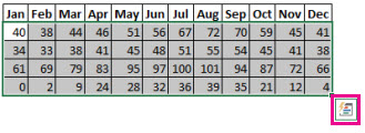
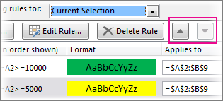
Use the Quick Analysis button  to apply selected conditional formatting to the selected data. The Quick Analysis button appears automatically when you select data.
-
Select the data that you want to conditionally format. The Quick Analysis button appears on the lower-right corner of the selection.

-
Click the Quick Analysis button
, or press Ctrl+Q. -
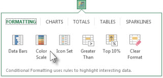
In the pop-up that appears, on the Formatting tab, move your mouse over the different options to see a Live Preview on your data, and then click on the formatting option you want.
Notes:
-
The formatting options that appear in the Formatting tab depend on the data you have selected. If your selection contains only text, then the available options are Text, Duplicate, Unique, Equal To, and Clear. When the selection contains only numbers, or both text and numbers, then the options are Data Bars, Colors, Icon Sets, Greater, Top 10%, and Clear.
-
Live preview will only render for those formatting options that can be used on your data. For example, if your selected cells don’t contain matching data and you select Duplicate, the live preview will not work.
-
-
If the Text that Contains dialog box appears, enter the formatting option you want to apply and click OK.
If you’d like to watch a video that shows how to use Quick Analysis to apply conditional formatting, see Video: Use conditional formatting.
You can download a sample workbook that contains different examples of applying conditional formatting, both with standard rules such as top and bottom, duplicates, Data Bars, Icon Sets and Color Scales, as well as manually creating rules of your own.
Download: Conditional formatting examples in Excel
Color scales are visual guides that help you understand data distribution and variation. A two-color scale helps you compare a range of cells by using a gradation of two colors. The shade of the color represents higher or lower values. For example, in a green and yellow color scale, as shown below, you can specify that higher value cells have a more green color and lower value cells have a more yellow color.
Tip: You can sort cells that have this format by their color — just use the context menu.
Tip: If any cells in the selection contain a formula that returns an error, the conditional formatting is not applied to those cells. To ensure that the conditional formatting is applied to those cells, use an IS or IFERROR function to return a value other than an error value.
Quick formatting
-
Select one or more cells in a range, table, or PivotTable report.
-
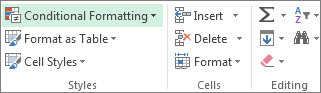
On the Home tab, in the Styles group, click the arrow next to Conditional Formatting, and then click Color Scales.
-
Select a two-color scale.
Hover over the color scale icons to see which icon is a two-color scale. The top color represents higher values, and the bottom color represents lower values.
You can change the method of scoping for fields in the Values area of a PivotTable report by using the Formatting Options button that appears next to a PivotTable field that has conditional formatting applied.
Advanced formatting
-
Select one or more cells in a range, table, or PivotTable report.
-
On the Home tab, in the Styles group, click the arrow next to Conditional Formatting, and then click Manage Rules. The Conditional Formatting Rules Manager dialog box appears.
-
Do one of the following:
-
To add a completely new conditional format, click New Rule. The New Formatting Rule dialog box appears.
-
To add a new conditional format based on one that is already listed, select the rule, then click Duplicate Rule. The duplicate rule appears in the dialog box. Select the duplicate, then select Edit Rule. The Edit Formatting Rule dialog box appears.
-
To change a conditional format, do the following:
-
Make sure that the appropriate worksheet, table, or PivotTable report is selected in the Show formatting rules for list box.
-
Optionally, change the range of cells by clicking Collapse Dialog in the Applies to box to temporarily hide the dialog box, by selecting the new range of cells on the worksheet, and then by selecting Expand Dialog.
-
Select the rule, and then click Edit rule. The Edit Formatting Rule dialog box appears.
-
-
-
Under Apply Rule To, to optionally change the scope for fields in the Values area of a PivotTable report by:
-
Selection: Click Selected cells.
-
All cells for a Value label: Click All cells showing <Value label> values.
-
All cells for a Value label, excluding subtotals and the grand total: Click All cells showing <Value label> values for <Row Label>.
-
-
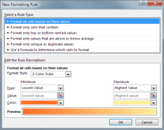
Under Select a Rule Type, click Format all cells based on their values (default).
-
Under Edit the Rule Description, in the Format Style list box, select 2-Color Scale.
-
To select a type in the Type box for Minimum and Maximum, do one of the following:
-
Format lowest and highest values: Select Lowest Value and Highest Value.
In this case, you do not enter a Minimum and MaximumValue.
-
Format a number, date, or time value: Select Number and then enter a Minimum and MaximumValue.
-
Format a percentage Percent: Enter a Minimum and MaximumValue.
Valid values are from 0 (zero) to 100. Don’t enter a percent sign.
Use a percentage when you want to visualize all values proportionally because the distribution of values is proportional.
-
Format a percentile: Select Percentile and then enter a Minimum and MaximumValue. Valid percentiles are from 0 (zero) to 100.
Use a percentile when you want to visualize a group of high values (such as the top 20thpercentile) in one color grade proportion and low values (such as the bottom 20th percentile) in another color grade proportion, because they represent extreme values that might skew the visualization of your data.
-
Format a formula result: Select Formula and then enter values for Minimum and Maximum.
-
The formula must return a number, date, or time value.
-
Start the formula with an equal sign (=).
-
Invalid formulas result in no formatting being applied.
-
It’s a good idea to test the formula to make sure that it doesn’t return an error value.
Notes:
-
Make sure that the Minimum value is less than the Maximum value.
-
You can choose a different type for the Minimum and Maximum. For example, you can choose a number for Minimum a percentage for Maximum.
-
-
-
-
To choose a Minimum and Maximum color scale, click Color for each, and then select a color.
If you want to choose additional colors or create a custom color, click More Colors. The color scale you select is shown in the Preview box.

Color scales are visual guides that help you understand data distribution and variation. A three-color scale helps you compare a range of cells by using a gradation of three colors. The shade of the color represents higher, middle, or lower values. For example, in a green, yellow, and red color scale, you can specify that higher value cells have a green color, middle value cells have a yellow color, and lower value cells have a red color.
Tip: You can sort cells that have this format by their color — just use the context menu.
Quick formatting
-
Select one or more cells in a range, table, or PivotTable report.
-
On the Home tab, in the Styles group, click the arrow next to Conditional Formatting, and then click Color Scales.
-
Select a three-color scale. The top color represents higher values, the center color represents middle values, and the bottom color represents lower values.
Hover over the color scale icons to see which icon is a three-color scale.
You can change the method of scoping for fields in the Values area of a PivotTable report by using the Formatting Options button that appears next to a PivotTable field that has conditional formatting applied..
Advanced formatting
-
Select one or more cells in a range, table, or PivotTable report.
-
On the Home tab, in the Styles group, click the arrow next to Conditional Formatting, and then click Manage Rules. The Conditional Formatting Rules Manager dialog box appears.
-
Do one of the following:
-
To add a new conditional format, click New Rule. The New Formatting Rule dialog box appears.
-
To add a new conditional format based on one that is already listed, select the rule, then click Duplicate Rule. The duplicate rule is copied and appears in the dialog box. Select the duplicate, then select Edit Rule. The Edit Formatting Rule dialog box appears.
-
To change a conditional format, do the following:
-
Make sure that the appropriate worksheet, table, or PivotTable report is selected in the Show formatting rules for list box.
-
Optionally, change the range of cells by clicking Collapse Dialog in the Applies to box to temporarily hide the dialog box, by selecting the new range of cells on the worksheet, and then by selecting Expand Dialog.
-
Select the rule, and then click Edit rule. The Edit Formatting Rule dialog box appears.
-
-
-
Under Apply Rule To, to optionally change the scope for fields in the Values area of a PivotTable report by:
-
Selection: Click Just these cells.
-
Corresponding field: Click All <value field> cells with the same fields.
-
Value field: Click All <value field> cells.
-
-
Under Select a Rule Type, click Format all cells based on their values.
-
Under Edit the Rule Description, in the Format Style list box, select 3-Color Scale.
-
Select a type for Minimum, Midpoint, and Maximum. Do one of the following:
-
Format lowest and highest values: Select a Midpoint.
In this case, you do not enter a Lowest and HighestValue.
-
Format a number, date, or time value: Select Number and then enter a value for Minimum, Midpoint, and Maximum.
-
Format a percentage: Select Percent and then enter a value for Minimum, Midpoint, and Maximum. Valid values are from 0 (zero) to 100. Do not enter a percent (%) sign.
Use a percentage when you want to visualize all values proportionally, because using a percentage ensures that the distribution of values is proportional.
-
Format a percentile: Select Percentile and then enter a value for Minimum, Midpoint, and Maximum.
Valid percentiles are from 0 (zero) to 100.
Use a percentile when you want to visualize a group of high values (such as the top 20th percentile) in one color grade proportion and low values (such as the bottom 20th percentile) in another color grade proportion, because they represent extreme values that might skew the visualization of your data.
-
Format a formula result: Select Formula and then enter a value for Minimum, Midpoint, and Maximum.
The formula must return a number, date, or time value. Start the formula with an equal sign (=). Invalid formulas result in no formatting being applied. It’s a good idea to test the formula to make sure that it doesn’t return an error value.
Notes:
-
You can set minimum, midpoint, and maximum values for the range of cells. Make sure that the value in Minimum is less than the value in Midpoint, which in turn is less than the value in Maximum.
-
You can choose a different type for Minimum, Midpoint, and Maximum. For example, you can choose a Minimum number, Midpoint percentile, and Maximum percent.
-
In many cases, the default Midpoint value of 50 percent works best, but you can adjust this to fit unique requirements.
-
-
-
To choose a Minimum, Midpoint, and Maximum color scale, click Color for each, and then select a color.
-
To choose additional colors or create a custom color, click More Colors.
-
The color scale you select is shown in the Preview box.
-
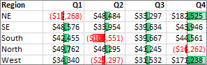
A data bar helps you see the value of a cell relative to other cells. The length of the data bar represents the value in the cell. A longer bar represents a higher value, and a shorter bar represents a lower value. Data bars are useful in spotting higher and lower numbers, especially with large amounts of data, such as top selling and bottom selling toys in a holiday sales report.
The example shown here uses data bars to highlight dramatic positive and negative values. You can format data bars so that the data bar starts in the middle of the cell, and stretches to the left for negative values.
Tip: If any cells in the range contain a formula that returns an error, the conditional formatting is not applied to those cells. To ensure that the conditional formatting is applied to those cells, use an IS or IFERROR function to return a value (such as 0 or «N/A») instead of an error value.
Quick formatting
-
Select one or more cells in a range, table, or PivotTable report.
-
On the Home tab, in the Style group, click the arrow next to Conditional Formatting, click Data Bars, and then select a data bar icon.
You can change the method of scoping for fields in the Values area of a PivotTable report by using the Apply formatting rule to option button.
Advanced formatting
-
Select one or more cells in a range, table, or PivotTable report.
-
On the Home tab, in the Styles group, click the arrow next to Conditional Formatting, and then click Manage Rules. The Conditional Formatting Rules Manager dialog box appears.
-
Do one of the following:
-
To add a conditional format, click New Rule. The New Formatting Rule dialog box appears.
-
To add a new conditional format based on one that is already listed, select the rule, then click Duplicate Rule. The duplicate rule is copied and appears in the dialog box. Select the duplicate, then select Edit Rule. The Edit Formatting Rule dialog box appears.
-
To change a conditional format, do the following:
-
-
Make sure that the appropriate worksheet, table, or PivotTable report is selected in the Show formatting rules for list box.
-
Optionally, change the range of cells by clicking Collapse Dialog in the Applies to box to temporarily hide the dialog box, by selecting the new range of cells on the worksheet, and then by selecting Expand Dialog.
-
Select the rule, and then click Edit rule. The Edit Formatting Rule dialog box appears.
-
-
-
Under Apply Rule To, to optionally change the scope for fields in the Values area of a PivotTable report by:
-
Selection: Click Just these cells.
-
Corresponding field: Click All <value field> cells with the same fields.
-
Value field: Click All <value field> cells.
-
-
Under Select a Rule Type, click Format all cells based on their values.
-
Under Edit the Rule Description, in the Format Style list box, select Data Bar.
-
Select a Minimum and MaximumType. Do one of the following:
-
Format lowest and highest values: Select Lowest Value and Highest Value.
In this case, you do not enter a value for Minimum and Maximum.
-
Format a number, date, or time value: Select Number and then enter a Minimum and MaximumValue.
-
Format a percentage: Select Percent and then enter a value for Minimum and Maximum.
Valid values are from 0 (zero) to 100. Do not enter a percent (%) sign.
Use a percentage when you want to visualize all values proportionally, because using a percentage ensures that the distribution of values is proportional.
-
Format a percentile Select Percentile and then enter a value for Minimum and Maximum.
Valid percentiles are from 0 (zero) to 100.
Use a percentile when you want to visualize a group of high values (such as the top 20th percentile) in one data bar proportion and low values (such as the bottom 20th percentile) in another data bar proportion, because they represent extreme values that might skew the visualization of your data.
-
Format a formula result Select Formula, and then enter a value for Minimum and Maximum.
-
The formula has to return a number, date, or time value.
-
Start the formula with an equal sign (=).
-
Invalid formulas result in no formatting being applied.
-
It’s a good idea to test the formula to make sure that it doesn’t return an error value.
-
Notes:
-
Make sure that the Minimum value is less than the Maximum value.
-
You can choose a different type for Minimum and Maximum. For example, you can choose a Minimum number and a Maximum percent.
-
-
To choose a Minimum and Maximum color scale, click Bar Color.
If you want to choose additional colors or create a custom color, click More Colors. The bar color you select is shown in the Preview box.
-
To show only the data bar and not the value in the cell, select Show Bar Only.
-
To apply a solid border to data bars, select Solid Border in the Border list box and choose a color for the border.
-
To choose between a solid bar and a gradiated bar, choose Solid Fill or Gradient Fill in the Fill list box.
-
To format negative bars, click Negative Value and Axis and then, in the Negative Value and Axis Settings dialog box, choose options for the negative bar fill and border colors. You can choose position settings and a color for the axis. When you are finished selecting options, click OK.
-
You can change the direction of bars by choosing a setting in the Bar Direction list box. This is set to Context by default, but you can choose between a left-to-right and a right-to-left direction, depending on how you want to present your data.
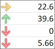
Use an icon set to annotate and classify data into three to five categories separated by a threshold value. Each icon represents a range of values. For example, in the 3 Arrows icon set, the green up arrow represents higher values, the yellow sideways arrow represents middle values, and the red down arrow represents lower values.
Tip: You can sort cells that have this format by their icon — just use the context menu.
The example shown here works with several examples of conditional formatting icon sets.

You can choose to show icons only for cells that meet a condition; for example, displaying a warning icon for those cells that fall below a critical value and no icons for those that exceed it. To do this, you hide icons by selecting No Cell Icon from the icon drop-down list next to the icon when you are setting conditions. You can also create your own combination of icon sets; for example, a green «symbol» check mark, a yellow «traffic light», and a red «flag.»
Tip: If any cells in the selection contain a formula that returns an error, the conditional formatting is not applied to those cells. To ensure that the conditional formatting is applied to those cells, use an IS or IFERROR function to return a value (such as 0 or «N/A») instead of an error value.
Quick formatting
-
Select the cells that you want to conditionally format.
-
On the Home tab, in the Style group, click the arrow next to Conditional Formatting, click Icon Set, and then select an icon set.
You can change the method of scoping for fields in the Values area of a PivotTable report by using the Apply formatting rule to option button.
Advanced formatting
-
Select the cells that you want to conditionally format.
-
On the Home tab, in the Styles group, click the arrow next to Conditional Formatting, and then click Manage Rules. The Conditional Formatting Rules Manager dialog box appears.
-
Do one of the following:
-
To add a conditional format, click New Rule. The New Formatting Rule dialog box appears.
-
To add a new conditional format based on one that is already listed, select the rule, then click Duplicate Rule. The duplicate rule is copied and appears in the dialog box. Select the duplicate, then select Edit Rule. The Edit Formatting Rule dialog box appears.
-
To change a conditional format, do the following:
-
Make sure that the appropriate worksheet, table, or PivotTable report is selected in the Show formatting rules for list box.
-
Optionally, change the range of cells by clicking Collapse Dialog in the Applies to box to temporarily hide the dialog box, by selecting the new range of cells on the worksheet, and then by selecting Expand Dialog.
-
Select the rule, and then click Edit rule. The Edit Formatting Rule dialog box appears.
-
-
-
Under Apply Rule To, to optionally change the scope for fields in the Values area of a PivotTable report by:
-
Selection: Click Just these cells.
-
Corresponding field: Click All <value field> cells with the same fields.
-
Value field: Click All <value field> cells.
-
-
Under Select a Rule Type, click Format all cells based on their values.
-
Under Edit the Rule Description, in the Format Style list box, select Icon Set.
-
Select an icon set. The default is 3 Traffic Lights (Unrimmed). The number of icons and the default comparison operators and threshold values for each icon can vary for each icon set.
-
You can adjust the comparison operators and threshold values. The default range of values for each icon are equal in size, but you can adjust these to fit your unique requirements. Make sure that the thresholds are in a logical sequence of highest to lowest from top to bottom.
-
Do one of the following:
-
Format a number, date, or time value: Select Number.
-
Format a percentage: Select Percent.
Valid values are from 0 (zero) to 100. Do not enter a percent (%) sign.
Use a percentage when you want to visualize all values proportionally, because using a percentage ensures that the distribution of values is proportional.
-
Format a percentile: Select Percentile. Valid percentiles are from 0 (zero) to 100.
Use a percentile when you want to visualize a group of high values (such as the top 20th percentile) using a particular icon and low values (such as the bottom 20th percentile) using another icon, because they represent extreme values that might skew the visualization of your data.
-
Format a formula result: Select Formula, and then enter a formula in each Value box.
-
The formula must return a number, date, or time value.
-
Start the formula with an equal sign (=).
-
Invalid formulas result in no formatting being applied.
-
It’s a good idea to test the formula to make sure that it doesn’t return an error value.
-
-
-
To make the first icon represent lower values and the last icon represent higher values, select Reverse Icon Order.
-
To show only the icon and not the value in the cell, select Show Icon Only.
Notes:
-
You may need to adjust the column width to accommodate the icon.
-
The size of the icon shown depends on the font size that is used in that cell. As the size of the font is increased, the size of the icon increases proportionally.
-
-
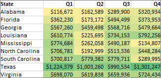
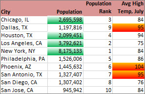
To more easily find specific cells, you can format them by using a comparison operator. For example, in an inventory worksheet sorted by categories, you could highlight products with fewer than 10 items on hand in yellow. Or, in a retail store summary worksheet, you might identify all stores with profits greater than 10%, sales volumes less than $100,000, and region equal to «SouthEast.»
The examples shown here work with examples of built-in conditional formatting criteria, such as Greater Than, and Top %. This formats cities with a population greater than 2,000,000 with a green background and average high temperatures in the top 30% with orange.
Note: You cannot conditionally format fields in the Values area of a PivotTable report by text or by date, only by number.
Quick formatting
-
Select one or more cells in a range, table, or PivotTable report.
-
On the Home tab, in the Style group, click the arrow next to Conditional Formatting, and then click Highlight Cells Rules.
-
Select the command you want, such as Between, Equal To Text that Contains, or A Date Occurring.
-
Enter the values you want to use, and then select a format.
You can change the method of scoping for fields in the Values area of a PivotTable report by using the Apply formatting rule to option button.
If you’d like to watch videos of these techniques, see Video: Conditionally format text and Video: Conditionally format dates.
Advanced formatting
-
Select one or more cells in a range, table, or PivotTable report.
-
On the Home tab, in the Styles group, click the arrow next to Conditional Formatting, and then click Manage Rules. The Conditional Formatting Rules Manager dialog box appears.
-
Do one of the following:
-
To add a conditional format, click New Rule. The New Formatting Rule dialog box appears.
-
To add a new conditional format based on one that is already listed, select the rule, then click Duplicate Rule. The duplicate rule is copied and appears in the dialog box. Select the duplicate, then select Edit Rule. The Edit Formatting Rule dialog box appears.
-
To change a conditional format, do the following:
-
-
Make sure that the appropriate worksheet, table, or PivotTable report is selected in the Show formatting rules for list box.
-
Optionally, change the range of cells by clicking Collapse Dialog in the Applies to box to temporarily hide the dialog box, by selecting the new range of cells on the worksheet or on other worksheets, and then by selecting Expand Dialog.
-
Select the rule, and then click Edit rule. The Edit Formatting Rule dialog box appears.
-
-
-
Under Apply Rule To, to optionally change the scope for fields in the Values area of a PivotTable report by:
-
Selection: Click Just these cells.
-
Corresponding field: Click All <value field> cells with the same fields.
-
Value field: Click All <value field> cells.
-
-
Under Select a Rule Type, click Format only cells that contain.
-
Under Edit the Rule Description, in the Format only cells with list box, do one of the following:
-
Format by number, date, or time: Select Cell Value, select a comparison operator, and then enter a number, date, or time.
For example, select Between and then enter 100 and 200, or select Equal to and then enter 1/1/2009.
You can also enter a formula that returns a number, date, or time value.
-
If you enter a formula, start it with an equal sign (=).
-
Invalid formulas result in no formatting being applied.
-
It’s a good idea to test the formula to make sure that it doesn’t return an error value.
-
-
Format by text: Select Specific Text, choosing a comparison operator, and then enter text.
For example, select Contains and then enter Silver, or select Starting with and then enter Tri.
Quotes are included in the search string, and you may use wildcard characters. The maximum length of a string is 255 characters.
You can also enter a formula that returns text.
-
If you enter a formula, start it with an equal sign (=).
-
Invalid formulas result in no formatting being applied.
-
It’s a good idea to test the formula to make sure that it doesn’t return an error value.
To see a video of this technique, see Video: Conditionally format text.
-
-
Format by date: Select Dates Occurring and then select a date comparison.
For example, select Yesterday or Next week.
To see a video of this technique, see Video: Conditionally format dates.
-
Format cells with blanks or no blanks: Select Blanks or No Blanks.
A blank value is a cell that contains no data and is different from a cell that contains one or more spaces (spaces are considered as text).
-
Format cells with error or no error values: Select Errors or No Errors.
Error values include: #####, #VALUE!, #DIV/0!, #NAME?, #N/A, #REF!, #NUM!, and #NULL!.
-
-
To specify a format, click Format. The Format Cells dialog box appears.
-
Select the number, font, border, or fill format you want to apply when the cell value meets the condition, and then click OK.
You can choose more than one format. The formats you select are shown in the Preview box.
You can find the highest and lowest values in a range of cells that are based on a cutoff value you specify. For example, you can find the top 5 selling products in a regional report, the bottom 15% products in a customer survey, or the top 25 salaries in a department .
Quick formatting
-
Select one or more cells in a range, table, or PivotTable report.
-
On the Home tab, in the Style group, click the arrow next to Conditional Formatting, and then click Top/Bottom Rules.
-
Select the command you want, such as Top 10 items or Bottom 10 %.
-
Enter the values you want to use, and then select a format.
You can change the method of scoping for fields in the Values area of a PivotTable report by using the Apply formatting rule to option button.
Advanced formatting
-
Select one or more cells in a range, table, or PivotTable report.
-
On the Home tab, in the Styles group, click the arrow next to Conditional Formatting, and then click Manage Rules. The Conditional Formatting Rules Manager dialog box appears.
-
Do one of the following:
-
To add a conditional format, click New Rule. The New Formatting Rule dialog box appears.
-
To add a new conditional format based on one that is already listed, select the rule, then click Duplicate Rule. The duplicate rule is copied and appears in the dialog box. Select the duplicate, then select Edit Rule. The Edit Formatting Rule dialog box appears.
-
To change a conditional format, do the following:
-
-
Make sure that the appropriate worksheet, table, or PivotTable report is selected in the Show formatting rules for list box.
-
Optionally, change the range of cells by clicking Collapse Dialog in the Applies to box to temporarily hide the dialog box, by selecting the new range of cells on the worksheet, and then by selecting Expand Dialog.
-
Select the rule, and then click Edit rule. The Edit Formatting Rule dialog box appears.
-
-
-
Under Apply Rule To, to optionally change the scope fields in the Values area of a PivotTable report by:
-
Selection: Click Just these cells.
-
Corresponding field: Click All <value field> cells with the same fields.
-
Value field: Click All <value field> cells.
-
-
Under Select a Rule Type, click Format only top or bottom ranked values.
-
Under Edit the Rule Description, in the Format values that rank in the list box, select Top or Bottom.
-
Do one of the following:
-
To specify a top or bottom number, enter a number and then clear the % of the selected range box. Valid values are 1 to 1000.
-
To specify a top or bottom percentage, enter a number and then select the % of the selected range box. Valid values are 1 to 100.
-
-
Optionally, change how the format is applied for fields in the Values area of a PivotTable report that are scoped by corresponding field.
By default, the conditional format is based on all visible values. However when you scope by corresponding field, instead of using all visible values, you can apply the conditional format for each combination of:
-
A column and its parent row field, by selecting each Column group.
-
A row and its parent column field, by selecting each Row group.
-
-
To specify a format, click Format. The Format Cells dialog box appears.
-
Select the number, font, border, or fill format you want to apply when the cell value meets the condition, and then click OK.
You can choose more than one format. The formats you select are shown in the Preview box.
You can find values above or below an average or standard deviation in a range of cells. For example, you can find the above average performers in an annual performance review or you can locate manufactured materials that fall below two standard deviations in a quality rating.
Quick formatting
-
Select one or more cells in a range, table, or PivotTable report.
-
On the Home tab, in the Style group, click the arrow next to Conditional Formatting, and then click Top/Bottom Rules.
-
Select the command you want, such as Above Average or Below Average.
-
Enter the values you want to use, and then select a format.
You can change the method of scoping for fields in the Values area of a PivotTable report by using the Apply formatting rule to option button.
Advanced formatting
-
Select one or more cells in a range, table, or PivotTable report.
-
On the Home tab, in the Styles group, click the arrow next to Conditional Formatting, and then click Manage Rules. The Conditional Formatting Rules Manager dialog box appears.
-
Do one of the following:
-
To add a conditional format, click New Rule. The New Formatting Rule dialog box appears.
-
To add a new conditional format based on one that is already listed, select the rule, then click Duplicate Rule. The duplicate rule is copied and appears in the dialog box. Select the duplicate, then select Edit Rule. The Edit Formatting Rule dialog box appears.
-
To change a conditional format, do the following:
-
-
Make sure that the appropriate worksheet, table, or PivotTable report is selected in the Show formatting rules for list box.
-
Optionally, change the range of cells by clicking Collapse Dialog in the Applies to box to temporarily hide the dialog box, by selecting the new range of cells on the worksheet, and then by selecting Expand Dialog.
-
Select the rule, and then click Edit rule. The Edit Formatting Rule dialog box appears.
-
-
-
Under Apply Rule To, to optionally change the scope for fields in the Values area of a PivotTable report by:
-
Selection: Click Just these cells.
-
Corresponding field: Click All <value field> cells with the same fields.
-
Value field: Click All <value field> cells.
-
-
Under Select a Rule Type, click Format only values that are above or below average.
-
Under Edit the Rule Description, in the Format values that are list box, do one of the following:
-
To format cells that are above or below the average for all of the cells in the range, select Above or Below.
-
To format cells that are above or below one, two, or three standard deviations for all of the cells in the range, select a standard deviation.
-
-
Optionally, change how the format is applied for fields in the Values area of a PivotTable report that are scoped by corresponding field.
By default, the conditionally format is based on all visible values. However when you scope by corresponding field, instead of using all visible values, you can apply the conditional format for each combination of:
-
A column and its parent row field, by selecting each Column group.
-
A row and its parent column field, by selecting each Row group.
-
-
Click Format to display the Format Cells dialog box.
-
Select the number, font, border, or fill format you want to apply when the cell value meets the condition, and then click OK.
You can choose more than one format. The formats you select are displayed in the Preview box.
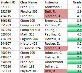
Note: You can’t conditionally format fields in the Values area of a PivotTable report by unique or duplicate values.
In the example shown here, conditional formatting is used on the Instructor column to find instructors that are teaching more than one class (duplicate instructor names are highlighted in a pale red color). Grade values that are found just once in the Grade column (unique values) are highlighted in a green color.
Quick formatting
-
Select the cells that you want to conditionally format.
-
On the Home tab, in the Style group, click the arrow next to Conditional Formatting, and then click Highlight Cells Rules.
-
Select Duplicate Values.
-
Enter the values you want to use, and then select a format.
Advanced formatting
-
Select the cells that you want to conditionally format.
-
On the Home tab, in the Styles group, click the arrow next to Conditional Formatting, and then click Manage Rules. The Conditional Formatting Rules Manager dialog box appears.
-
Do one of the following:
-
To add a conditional format, click New Rule. The New Formatting Rule dialog box appears.
-
To add a new conditional format based on one that is already listed, select the rule, then click Duplicate Rule. The duplicate rule is copied and appears in the dialog box. Select the duplicate, then select Edit Rule. The Edit Formatting Rule dialog box appears.
-
To change a conditional format, do the following:
-
-
Make sure that the appropriate worksheet or table is selected in the Show formatting rules for list box.
-
Optionally, change the range of cells by clicking Collapse Dialog in the Applies to box to temporarily hide the dialog box, by selecting the new range of cells on the worksheet, and then by selecting Expand Dialog.
-
Select the rule, and then click Edit rule. The Edit Formatting Rule dialog box appears.
-
-
-
Under Select a Rule Type, click Format only unique or duplicate values.
-
Under Edit the Rule Description, in the Format all list box, select unique or duplicate.
-
Click Format to display the Format Cells dialog box.
-
Select the number, font, border, or fill format you want to apply when the cell value meets the condition, and then click OK.
You can choose more than one format. The formats you select are shown in the Preview box.
If none of the above options is what you’re looking for, you can create your own conditional formatting rule in a few simple steps.
Notes: If there’s already a rule defined that you just want to work a bit differently, duplicate the rule and edit it.
-
Select Home > Conditional Formatting > Manage Rules, then in the Conditional Formatting Rule Manager dialog, select a listed rule and then select Duplicate Rule. The duplicate rule then appears in the list.
-
Select the duplicate rule, then select Edit Rule.
-
Select the cells that you want to format.
-
On the Home tab, click Conditional Formatting > New Rule.
-
Create your rule and specify its format options, then click OK.
If you don’t see the options that you want, you can use a formula to determine which cells to format — see the next section for steps).
If you don’t see the exact options you need when you create your own conditional formatting rule, you can use a logical formula to specify the formatting criteria. For example, you may want to compare values in a selection to a result returned by a function or evaluate data in cells outside the selected range, which can be in another worksheet in the same workbook. Your formula must return True or False (1 or 0), but you can use conditional logic to string together a set of corresponding conditional formats, such as different colors for each of a small set of text values (for example, product category names).
Note: You can enter cell references in a formula by selecting cells directly on a worksheet or other worksheets. Selecting cells on the worksheet inserts absolute cell references. If you want Excel to adjust the references for each cell in the selected range, use relative cell references. For more information, see Create or change a cell reference and Switch between relative, absolute, and mixed references.
Tip: If any cells contain a formula that returns an error, conditional formatting is not applied to those cells. To address this, use IS functions or an IFERROR function in your formula to return a value that you specify (such as 0, or «N/A») instead of an error value.
-
On the Home tab, in the Styles group, click the arrow next to Conditional Formatting, and then click Manage Rules.
The Conditional Formatting Rules Manager dialog box appears.
-
Do one of the following:
-
To add a conditional format, click New Rule. The New Formatting Rule dialog box appears.
-
To add a new conditional format based on one that is already listed, select the rule, then click Duplicate Rule. The duplicate rule is copied and appears in the dialog box. Select the duplicate, then select Edit Rule. The Edit Formatting Rule dialog box appears.
-
To change a conditional format, do the following:
-
-
Make sure that the appropriate worksheet, table, or PivotTable report is selected in the Show formatting rules for list box.
-
Optionally, change the range of cells by clicking Collapse Dialog in the Applies to box to temporarily hide the dialog box, by selecting the new range of cells on the worksheet or other worksheets, and then by clicking Expand Dialog.
-
Select the rule, and then click Edit rule. The Edit Formatting Rule dialog box appears.
-
-
-
Under Apply Rule To, to optionally change the scope for fields in the Values area of a PivotTable report, do the following:
-
To scope by selection: Click Selected cells.
-
To scope by corresponding field: Click All cells showing <Values field> values.
-
To scope by Value field: Click All cells showing <Values field> for <Row>.
-
-
Under Select a Rule Type, click Use a formula to determine which cells to format.
-
Under Edit the Rule Description, in the Format values where this formula is true list box, enter a formula.
You have to start the formula with an equal sign (=), and the formula must return a logical value of TRUE (1) or FALSE (0).
-
Click Format to display the Format Cells dialog box.
-
Select the number, font, border, or fill format you want to apply when the cell value meets the condition, and then click OK.
You can choose more than one format. The formats you select are shown in the Preview box.
Example 1: Use two conditional formats with criteria that uses AND and OR tests
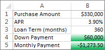
The following example shows the use of two conditional formatting rules. If the first rule doesn’t apply, the second rule applies.
First rule: a home buyer has budgeted up to $75,000 as a down payment and $1,500 per month as a mortgage payment. If both the down payment and the monthly payments fit these requirements, cells B4 and B5 are formatted green.
Second rule: if either the down payment or the monthly payment doesn’t meet the buyer’s budget, B4 and B5 are formatted red. Change some values, such as the APR, the loan term, the down payment, and the purchase amount to see what happens with the conditionally formatted cells.
Formula for first rule (applies green color)
=AND(IF($B$4<=75000,1),IF(ABS($B$5)<=1500,1))
Formula for second rule (applies red color)
=OR(IF($B$4>=75000,1),IF(ABS($B$5)>=1500,1))
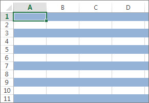
Example 2: Shade every other row by using the MOD and ROW functions
A conditional format applied to every cell in this worksheet shades every other row in the range of cells with a blue cell color. You can select all cells in a worksheet by clicking the square above row 1 and to the left of column A. The MOD function returns a remainder after a number (the first argument) is divided by divisor (the second argument). The ROW function returns the current row number. When you divide the current row number by 2, you always get either a 0 remainder for an even number or a 1 remainder for an odd number. Because 0 is FALSE and 1 is TRUE, every odd numbered row is formatted. The rule uses this formula: =MOD(ROW(),2)=1.
Note: You can enter cell references in a formula by selecting cells directly on a worksheet or other worksheets. Selecting cells on the worksheet inserts absolute cell references. If you want Excel to adjust the references for each cell in the selected range, use relative cell references. For more information, see Create or change a cell reference and Switch between relative, absolute, and mixed references.
-
The following video shows you the basics of using formulas with conditional formatting.
If you want to apply an existing formatting style to new or other data on your worksheet, you can use Format Painter to copy the conditional formatting to that data.
-
Click the cell that has the conditional formatting that you want to copy.
-
Click Home > Format Painter.
The pointer changes to a paintbrush.
Tip: You can double-click Format Painter if you want to keep using the paintbrush to paste the conditional formatting in other cells.
-
To paste the conditional formatting, drag the paintbrush across the cells or ranges of cells you want to format.
-
To stop using the paintbrush, press Esc.

Note: If you’ve used a formula in the rule that applies the conditional formatting, you might have to adjust any cell references in the formula after pasting the conditional format. For more information, see Switch between relative, absolute, and mixed references.
If your worksheet contains conditional formatting, you can quickly locate the cells so that you can copy, change, or delete the conditional formats. Use the Go To Special command to find only cells with a specific conditional format, or to find all cells that have conditional formats.
Find all cells that have a conditional format
-
Click any cell that does not have a conditional format.
-
On the Home tab, in the Editing group, click the arrow next to Find & Select, and then click Conditional Formatting.
Find only cells that have the same conditional format
-
Click any cell that has the conditional format that you want to find.
-
On the Home tab, in the Editing group, click the arrow next to Find & Select, and then click Go To Special.
-
Click Conditional formats.
-
Click Same under Data validation.
When you use conditional formatting, you set up rules that Excel uses to determine when to apply the conditional formatting. To manage these rules, you should understand the order in which these rules are evaluated, what happens when two or more rules conflict, how copying and pasting can affect rule evaluation, how to change the order in which rules are evaluated, and when to stop rule evaluation.
-
Learn about conditional formatting rule precedence
You create, edit, delete, and view all conditional formatting rules in the workbook by using the Conditional Formatting Rules Manager dialog box. (On the Home tab, click Conditional Formatting, and then click Manage Rules.)
The Conditional Formatting Rules Manager dialog box appears.
When two or more conditional formatting rules apply, these rules are evaluated in order of precedence (top to bottom) by how they are listed in this dialog box.
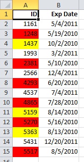
Here’s an example that has expiration dates for ID badges. We want to mark badges that expire within 60 days but are not yet expired with a yellow background color, and expired badges with a red background color.
In this example, cells with employee ID numbers who have certification dates due to expire within 60 days are formatted in yellow, and ID numbers of employees with an expired certification are formatted in red. The rules are shown in the following image.
The first rule (which, if True, sets cell background color to red) tests a date value in column B against the current date (obtained by using the TODAY function in a formula). Assign the formula to the first data value in column B, which is B2. The formula for this rule is =B2<TODAY(). This formula tests the cells in column B (cells B2:B15). If the formula for any cell in column B evaluates to True, its corresponding cell in column A (for example, A5 corresponds to B5, A11 corresponds to B11), is then formatted with a red background color. After all the cells specified under Applies to are evaluated with this first rule, the second rule is tested. This formula checks if values in the B column are less than 60 days from the current date (for example, suppose today’s date is 8/11/2010). The cell in B4, 10/4/2010, is less than 60 days from today, so it evaluates as True, and is formatted with a yellow background color. The formula for this rule is =B2<TODAY()+60. Any cell that was first formatted red by the highest rule in the list is left alone.
A rule higher in the list has greater precedence than a rule lower in the list. By default, new rules are always added to the top of the list and therefore have a higher precedence, so you’ll want to keep an eye on their order. You can change the order of precedence by using the Move Up and Move Down arrows in the dialog box.
-
What happens when more than one conditional formatting rule evaluates to True
Sometimes you have more than one conditional formatting rule that evaluates to True. Here’s how rules are applied, first when rules don’t conflict, and then when they do conflict:
When rules don’t conflict For example, if one rule formats a cell with a bold font and another rule formats the same cell with a red color, the cell is formatted with both a bold font and a red color. Because there is no conflict between the two formats, both rules are applied.
When rules conflict For example, one rule sets a cell font color to red and another rule sets a cell font color to green. Because the two rules are in conflict, only one can apply. The rule that is applied is the one that is higher in precedence (higher in the list in the dialog box).
-
How pasting, filling, and the Format Painter affect conditional formatting rules
While editing your worksheet, you may copy and paste cell values that have conditional formats, fill a range of cells with conditional formats, or use the Format Painter. These operations can affect conditional formatting rule precedence in the following way: a new conditional formatting rule based on the source cells is created for the destination cells.
If you copy and paste cell values that have conditional formats to a worksheet opened in another instance of Excel (another Excel.exe process running at the same time on the computer), no conditional formatting rule is created in the other instance and the format is not copied to that instance.
-
What happens when a conditional format and a manual format conflict
If a conditional formatting rule evaluates as True, it takes precedence over any existing manual format for the same selection. This means that if they conflict, the conditional formatting applies and the manual format does not. If you delete the conditional formatting rule, the manual formatting for the range of cells remains.
Manual formatting is not listed in the Conditional Formatting Rules Manager dialog box nor is it used to determine precedence.
-
Controlling when rule evaluation stops by using the Stop If True check box
For backwards compatibility with versions of Excel earlier than Excel 2007, you can select the Stop If True check box in the Manage Rules dialog box to simulate how conditional formatting might appear in those earlier versions of Excel that do not support more than three conditional formatting rules or multiple rules applied to the same range.
For example, if you have more than three conditional formatting rules for a range of cells, and are working with a version of Excel earlier than Excel 2007, that version of Excel:
-
Evaluates only the first three rules.
-
Applies the first rule in precedence that is True.
-
Ignores rules lower in precedence if they are True.
The following table summarizes each possible condition for the first three rules:
If rule
Is
And if rule
Is
And if rule
Is
Then
One
True
Two
True or False
Three
True or False
Rule one is applied and rules two and three are ignored.
One
False
Two
True
Three
True or False
Rule two is applied and rule three is ignored.
One
False
Two
False
Three
True
Rule three is applied.
One
False
Two
False
Three
False
No rules are applied.
You can select or clear the Stop If True check box to change the default behavior:
-
To evaluate only the first rule, select the Stop If True check box for the first rule.
-
To evaluate only the first and second rules, select the Stop If True check box for the second rule.
You can’t select or clear the Stop If True check box if the rule formats by using a data bar, color scale, or icon set.
-

If you’d like to watch a video showing how to manage conditional formatting rules, see Video: Manage conditional formatting.
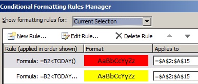
The order in which conditional formatting rules are evaluated — their precedence — also reflects their relative importance: the higher a rule is on the list of conditional formatting rules, the more important it is. This means that in cases where two conditional formatting rules conflict with each other, the rule that is higher on the list is applied and the rule that is lower on the list is not applied.
-
On the Home tab, in the Styles group, click the arrow next to Conditional Formatting, and then click Manage Rules.
The Conditional Formatting Rules Manager dialog box appears.
The conditional formatting rules for the current selection are displayed, including the rule type, the format, the range of cells the rule applies to, and the Stop If True setting.
If you don’t see the rule that you want, in the Show formatting rules for list box, make sure that the right range of cells, worksheet, table, or PivotTable report is selected.
-
Select a rule. Only one rule can be selected at a time.
-
To move the selected rule up in precedence, click Move Up. To move the selected rule down in precedence, click Move Down.
-
Optionally, to stop rule evaluation at a specific rule, select the Stop If True check box.
Clear conditional formatting on a worksheet
-
On the Home tab, click Conditional Formatting > Clear Rules > Clear Rules from Entire Sheet.
Follow these steps if you have conditional formatting in a worksheet, and you need to remove it.
For an entire
worksheet
-
On the Home tab, click Conditional Formatting > Clear Rules > Clear Rules from Entire Sheet.
In a range of cells
-
Select the cells that contain the conditional formatting.
-
Click the Quick Analysis Lens
button that appears to the bottom right of the selected data.Notes:
Quick Analysis Lens will not be visible if:-
All of the cells in the selected range are empty, or
-
There is an entry only in the upper-left cell of the selected range, with all of the other cells in the range being empty.
-
-
Click Clear Format.
 button that appears to the bottom right of the selected data.
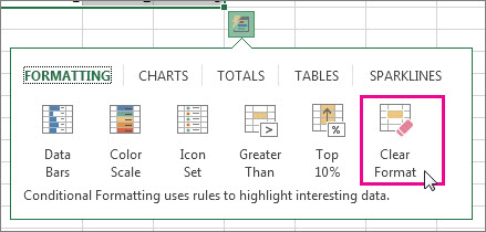
Find and remove the same conditional formats throughout a worksheet
-
Click on a cell that has the conditional format that you want to remove throughout the worksheet.
-
On the Home tab, click the arrow next to Find & Select, and then click Go To Special.
-
Click Conditional formats.
-
Click Same under Data validation. to select all of the cells that contain the same conditional formatting rules.
-
On the Home tab, click Conditional Formatting > Clear Rules > Clear Rules from Selected Cells.
Tip: The following sections use examples so you can follow along in Excel for the web. To start, download the Conditional Formatting Examples workbook and save it to OneDrive. Then, open OneDrive in a web browser and select the downloaded file.
-
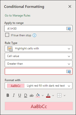
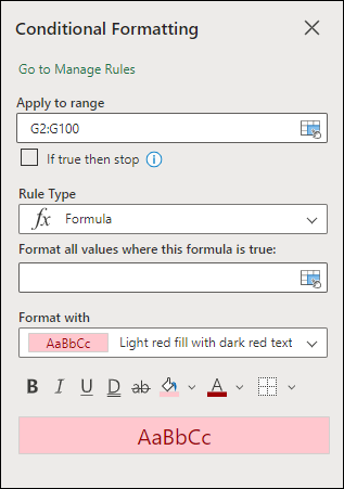
Select the cells you want to format, then select Home > Styles > Conditional Formatting > New Rule. You can also open the Conditional Formatting pane and create a new rule without first selecting a range of cells.
-
Verify or adjust the cells in Apply to range.
-
Choose a Rule Type and adjust the options to meet your needs.
-
When finished, select Done and the rule will be applied to your range.
-
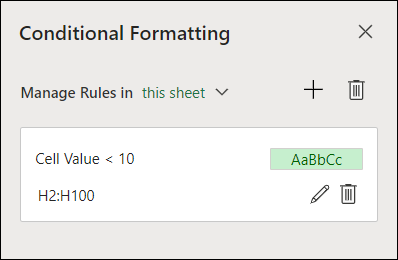
Select a cell which has a conditional format you want to change. Or you can select Home > Styles > Conditional Formatting > Manage Rules to open the Conditional Formatting task pane and select an existing rule.
-
The Conditional Formatting task pane displays any rules which apply to specific cells or ranges of cells.
-
Hover over the rule and select Edit by clicking the pencil icon. This opens the task pane for rule editing.
-
Modify the rule settings and click Done to apply the changes.
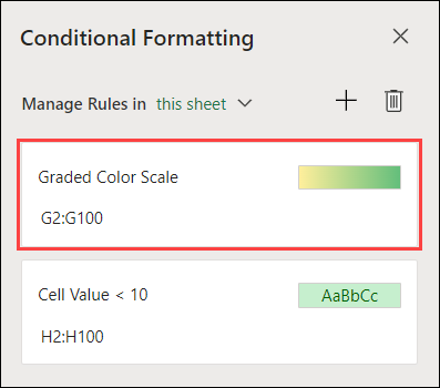
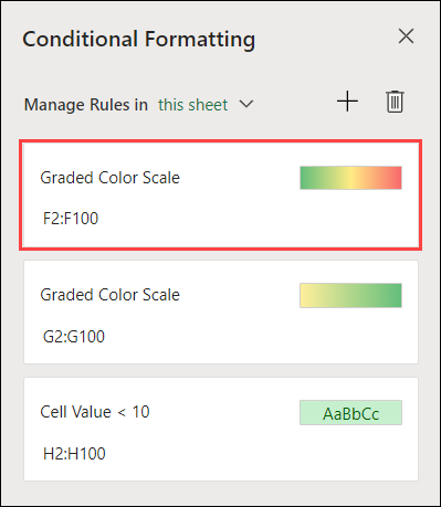
The Conditional Formatting task pane provides everything you need for creating, editing, and deleting rules. Use Manage Rules to open the task pane and work with all the Conditional Formatting rules in a selection or a sheet.
-
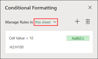
In an open workbook, select Home > Styles > Conditional Formatting > Manage Rules.
-
The Conditional Formatting task pane opens and displays the rules, scoped to your current selection.
From here, you can:
-
Choose a different scope on the Manage Rules in menu — for example, choosing this sheet tells Excel to look for all rules on the current sheet.
-
Add a rule by selecting New Rule (the plus sign).
-
Delete all rules in scope by selecting Delete All Rules (the garbage can).
You can use a formula to determine how Excel evaluates and formats a cell. Open the Conditional Formatting pane and select an existing rule or create a new rule.
In the Rule Type dropdown, select Formula.
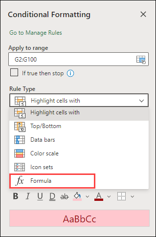
Enter the formula in the box. You can use any formula that returns a logical value of TRUE (1) or FALSE (0), but you can use AND and OR to combine a set of logical checks.
For example, =AND(B3=»Grain»,D3<500) is true for a cell in row 3 if both B3=»Grain» and D3<500 are true.
You can clear conditional formatting in selected cells or the entire worksheet.
-
To clear conditional formatting in selected cells, select the cells in the worksheet. Then Select Home > Styles > Conditional Formatting > Clear Rules > Clear Rules from Selected Cells.
-
To clear conditional formatting in the entire worksheet, select Home > Styles > Conditional Formatting > Clear Rules > Clear Rules from Entire Sheet.
-
To delete conditional formatting rules, select Home > Styles > Conditional Formatting >Manage Rules and use the delete (garbage can) on a specific rule or the Delete all rules button.
Color scales are visual guides which help you understand data distribution and variation. Excel offers both two-color scales and three-color scales.
A two-color scale helps you compare a range of cells by using a gradation of two colors. The shade of the color represents higher or lower values. For example, in a green and yellow color scale, you can specify that higher value cells be more green and lower value cells have a more yellow.
A three-color scale helps you compare a range of cells by using a gradation of three colors. The shade of the color represents higher, middle, or lower values. For example, in a green, yellow, and red color scale, you can specify that higher value cells have a green color, middle value cells have a yellow color, and lower value cells have a red color.
Tip: You can sort cells that have one of these formats by their color — just use the context menu.
-
Select the cells that you want to conditionally format using color scales.
-
Click Home > Styles > Conditional Formatting > Color Scales and select a color scale.
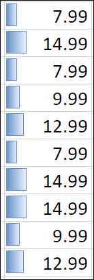
A data bar helps you see the value of a cell relative to other cells. The length of the data bar represents the value in the cell. A longer bar represents a higher value, and a shorter bar represents a lower value. Data bars are useful in spotting higher and lower numbers, especially with large amounts of data, such as top selling and bottom selling toys in a holiday sales report.
-
Select the cells that you want to conditionally format.
-
Select Home > Styles > Conditional Formatting > Data Bars and select a style.
Use an icon set to annotate and classify data into three to five categories separated by a threshold value. Each icon represents a range of values. For example, in the 3 Arrows icon set, the green up arrow represents higher values, the yellow sideways arrow represents middle values, and the red down arrow represents lower values.
-
Select the cells that you want to conditionally format.
-
Select Home > Styles > Conditional Formatting > Icon Sets and choose an icon set.
This option lets you highlight specific cell values within a range of cells based on their specific contents. This can be especially useful when working with data sorted using a different range.
For example, in an inventory worksheet sorted by categories, you could highlight the names of products where you have fewer than 10 items in stock so it’s easy to see which products need restocking without resorting the data.
-
Select the cells that you want to conditionally format.
-
Select Home > Styles > Conditional Formatting > Highlight Cell Rules.
-
Select the comparison, such as Between, Equal To, Text That Contains, or A Date Occurring.
You can highlight the highest and lowest values in a range of cells which are based on a specified cutoff value.
Some examples of this would include highlighting the top five selling products in a regional report, the bottom 15% products in a customer survey, or the top 25 salaries in a department.
-
Select the cells that you want to conditionally format.
-
Select Home > Styles > Conditional Formatting > Top/Bottom Rules.
-
Select the command you want, such as Top 10 items or Bottom 10 %.
-
Enter the values you want to use, and select a format (fill, text, or border color).
You can highlight values above or below an average or standard deviation in a range of cells.
For example, you can find the above-average performers in an annual performance review, or locate manufactured materials that fall below two standard deviations in a quality rating.
-
Select the cells that you want to conditionally format.
-
Select Home> Styles > Conditional Formatting > Top/Bottom Rules.
-
Select the option you want, such as Above Average or Below Average.
-
Enter the values you want to use, and select a format (fill, text, or border color).
-
Select the cells that you want to conditionally format.
-
Select Home > Styles > Conditional Formatting > Highlight Cell Rules > Duplicate Values.
-
Enter the values you want to use, and select a format (fill, text, or border color).
If you want to apply an existing formatting style to other cells on your worksheet, use Format Painter to copy the conditional formatting to that data.
-
Click the cell that has the conditional formatting you want to copy.
-
Click Home > Format Painter.
The pointer will change to a paintbrush.
Tip: You can double-click Format Painter if you want to keep using the paintbrush to paste the conditional formatting in other cells.
-
Drag the paintbrush across the cells or range of cells you want formatted.
-
To stop using the paintbrush, press Esc.
Note: If you’ve used a formula in the rule that applies the conditional formatting, you might have to adjust relative and absolute references in the formula after pasting the conditional format. For more information, see Switch between relative, absolute, and mixed references.
Note: You can’t use conditional formatting on external references to another workbook.
Need more help?
You can always ask an expert in the Excel Tech Community or get support in the Answers community.
See Also
Conditional formatting compatibility issues
This tutorial will demonstrate how to highlight cells depending on the answer returned by an IF statement formula using Conditional Formatting in Excel and Google Sheets.
Highlight Cells With Conditional Formatting
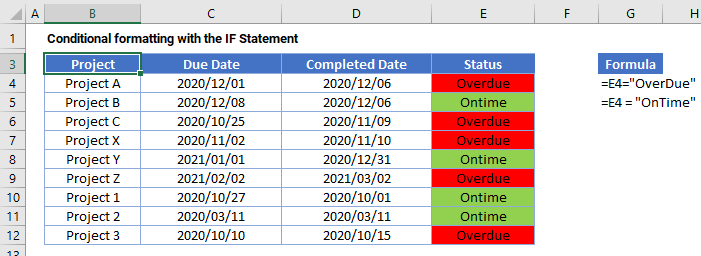
A cell can be formatted by conditional formatting based on the value returned by an IF statement on your Excel worksheet.
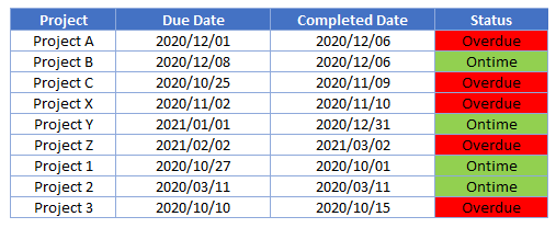
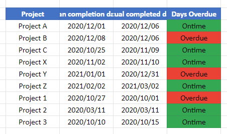
- First, create the IF statement in Column E.
=IF(D4>C4,”Overdue”,”Ontime”)
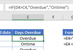
- This formula can be copied down to Row 12.
- Now, create a custom formula within the Conditional Formatting rule to set the background color of all the “Overdue” cells to red.
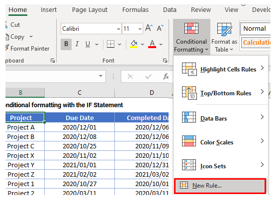
- Select the range you want to apply formatting to.
- In the Ribbon, select Home > Conditional Formatting > New Rule.
- Select Use a formula to determine which cells to format, and enter the formula:
=E4=”OverDue”
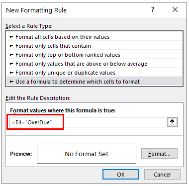
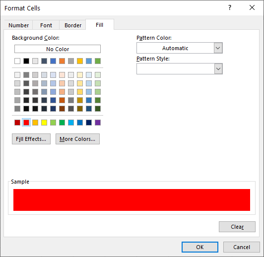
- Click on the Format button and select your desired formatting.
- Click OK, and then OK once again to return to the Conditional Formatting Rules Manager.
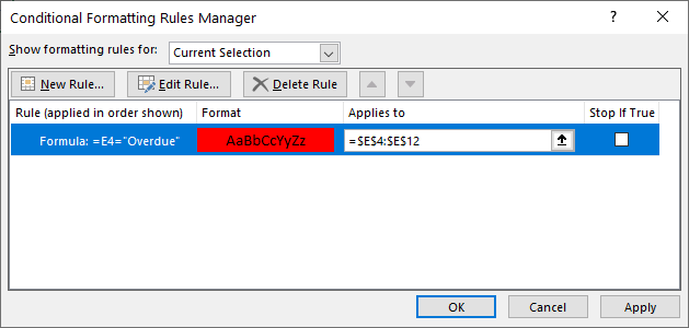
- Click Apply to apply the formatting to your selected range and then click Close.
The formula entered will return TRUE when the cell contains the word “Overdue” and will therefore format the text in those cells with a background color of red. - To format the “OnTime” cells to green, you can create another rule based on the same range of cells.
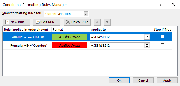
- Click Apply to apply to the range.
Highlight Cells If… in Google Sheets
The process to highlight cells that contain an IF Statement in Google Sheets is similar to the process in Excel.
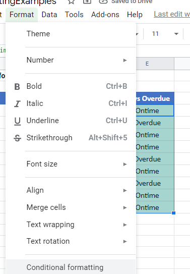
- Highlight the cells you wish to format, and then click on Format > Conditional Formatting.
- The Apply to Range section will already be filled in.

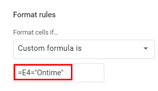
- From the Format Rules section, select Custom Formula and type in the formula.
- Select the fill style for the cells that meet the criteria.
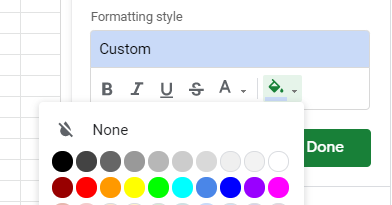
- Click Done to apply the rule.
 Please Note:
This article is written for users of the following Microsoft Excel versions: 2007 and 2010. If you are using an earlier version (Excel 2003 or earlier), this tip may not work for you. For a version of this tip written specifically for earlier versions of Excel, click here: Colors in an IF Function.
![]()
Written by Allen Wyatt (last updated June 21, 2018)
This tip applies to Excel 2007 and 2010
Steve would like to create an IF statement (using the worksheet function) based on the color of a cell. For example, if A1 has a green fill, he wants to return the word «go», if it has a red fill, he wants to return the word «stop», and if it is any other color return the word «neither». Steve prefers to not use a macro to do this.
Unfortunately, there is no way to acceptably accomplish this task without using macros, in one form or another. The closest non-macro solution is to create a name that determines colors, in this manner:
- Select cell A1.
- Click Insert | Name | Define. Excel displays the Define Name dialog box.
- Use a name such as «mycolor» (without the quote marks).
- In the Refers To box, enter the following, as a single line:
- Click OK.
     =IF(GET.CELL(38,Sheet1!A1)=10,"GO",IF(GET.CELL(38,Sheet1!A1)
     =3,"Stop","Neither"))
With this name defined, you can, in any cell, enter the following:
=mycolor
The result is that you will see text based upon the color of the cell in which you place this formula. The drawback to this approach, of course, is that it doesn’t allow you to reference cells other than the one in which the formula is placed.
The solution, then, is to use a user-defined function, which is (by definition) a macro. The macro can check the color with which a cell is filled and then return a value. For instance, the following example returns one of the three words, based on the color in a target cell:
Function CheckColor1(range)
    If range.Interior.Color = RGB(256, 0, 0) Then
        CheckColor1 = "Stop"
    ElseIf range.Interior.Color = RGB(0, 256, 0) Then
        CheckColor1 = "Go"
    Else
        CheckColor1 = "Neither"
    End If
End Function
This macro evaluates the RGB values of the colors in a cell, and returns a string based on those values. You could use the function in a cell in this manner:
=CheckColor1(B5)
If you prefer to check index colors instead of RGB colors, then the following variation will work:
Function CheckColor2(range)
    If range.Interior.ColorIndex = 3 Then
        CheckColor2 = "Stop"
    ElseIf range.Interior.ColorIndex = 4 Then
        CheckColor2 = "Go"
    Else
        CheckColor2 = "Neither"
    End If
End Function
Whether you are using the RGB approach or the color index approach, you’ll want to check to make sure that the values used in the macros reflect the actual values used for the colors in the cells you are testing. In other words, Excel allows you to use different shades of green and red, so you’ll want to make sure that the RGB values and color index values used in the macros match those used by the color shades in your cells.
One way you can do this is to use a very simple macro that does nothing but return a color index value:
Function GetFillColor(Rng As Range) As Long
    GetFillColor = Rng.Interior.ColorIndex
End Function
Now, in your worksheet, you can use the following:
=GetFillColor(B5)
The result is the color index value of cell B5 is displayed. Assuming that cell B5 is formatted using one of the colors you expect (red or green), you can plug the index value back into the earlier macros to get the desired results. You could simply skip that step, however, and rely on the value returned by GetFillColor to put together an IF formula, in this manner:
=IF(GetFillColor(B5)=4,"Go", IF(GetFillColor(B5)=3,"Stop", "Neither"))
You’ll want to keep in mind that these functions (whether you look at the RGB color values or the color index values) examine the explicit formatting of a cell. They don’t take into account any implicit formatting, such as that applied through conditional formatting.
For some other good ideas, formulas, and functions on working with colors, refer to this page at Chip Pearson’s website:
http://www.cpearson.com/excel/colors.aspx
If you would like to know how to use the macros described on this page (or on any other page on the ExcelTips sites), I’ve prepared a special page that includes helpful information. Click here to open that special page in a new browser tab.
ExcelTips is your source for cost-effective Microsoft Excel training.
This tip (10780) applies to Microsoft Excel 2007 and 2010. You can find a version of this tip for the older menu interface of Excel here: Colors in an IF Function.
Author Bio
With more than 50 non-fiction books and numerous magazine articles to his credit, Allen Wyatt is an internationally recognized author. He is president of Sharon Parq Associates, a computer and publishing services company. Learn more about Allen…
MORE FROM ALLEN
Copying Comments to Cells
Need to copy whatever is in a comment into a cell on your worksheet? If you have lots of comments, manually doing this …
Discover More
Stopping Date Parsing when Opening a CSV File
Excel tries to make sense out of any data that you import from a non-Excel file. Sometimes this can have unwanted …
Discover More
Determining the Complexity of a Worksheet
If you have multiple worksheets that each provide different ways to arrive at the same results, you may be wondering how …
Discover More
In this article we will learn how to color rows based on text criteria we use the “Conditional Formatting” option. This option is available in the “Home Tab” in the “Styles” group in Microsoft Excel.
Conditional Formatting in Excel is used to highlight the data on the basis of some criteria. It would be difficult to see various trends just for examining your Excel worksheet. Conditional Formatting in excel provides a way to visualize data and make worksheets easier to understand.
Excel Conditional Formatting allows you to apply formatting basis on the cell values such as colors, icons and data bars. For this, we will create a rule in excel Conditional Formatting based on cell value
How to write an if statement in excel?
IF function is used for logic_test and returns value on the basis of the result of the logic_test. Excel conditional formatting formula multiple conditions uses Statements like less than or equal to or greater than or equal to the value are used in IF formula
Syntax:
=IF (logical_test, [value_if_true], [value_if_false])
Let’s learn how to do conditional formatting in excel using IF function with the example.
Here is a list of Names and their respective Scores.
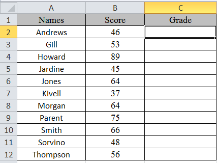
multiple if statements excel functions are used here. So, there are 3 results based on the condition. if then statements in excel is used via excel conditional formatting formula
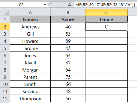
Write the formula in C2 cell.
Formula
=IF(B2<50,»C»,IF(B2<75,»B»,»A»))
Explanation:
IF function only returns 2 results, one [value_if_True] and Second [value-if_False]
First IF function checks, if the score is less than 50, would get C grade, The Second IF function tests if the score is less than 75 would get B grade and the rest A grade.
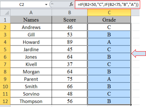
Copy the formula in other cells, select the cells taking the first cell where the formula is already applied, use shortcut key Ctrl + D
Now we will apply conditional formatting to it.
Select Home >Conditional Formatting > New Rule.
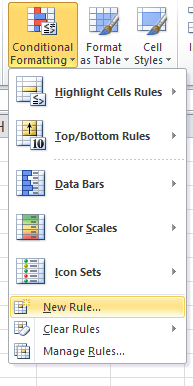
A dialog box appears
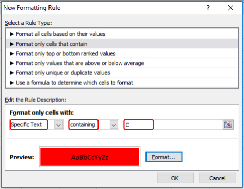
Select Format only cells that contain > Specific text in option list and write C as text to be formatted.
Fill Format with Red colour and click OK.
Now select the colour Yellow and Green for A and B respectively as done above for C.
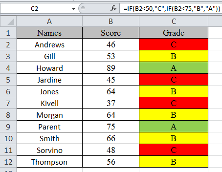
In this article, we used IF function and Conditional formatting tool to get highlighted grade.
As you can see excel change cell color based on value of another cell using IF function and Conditional formatting tool
Hope you learned how to use conditional formatting in Excel using IF function. Explore more conditional formulas in excel here. You can perform Conditional Formatting in Excel 2016, 2013 and 2010. If you have any unresolved query regarding this article, please do mention below. We will help you.
Related Articles:
How to use the Conditional formatting based on another cell value in Excel
How to use the Conditional Formatting using VBA in Microsoft Excel
How to use the Highlight cells that contain specific text in Excel
How to Sum Multiple Columns with Condition in Excel
Popular Articles:
50 Excel Shortcut to Increase Your Productivity
How to use the VLOOKUP Function in Excel
How to use the COUNTIF function in Excel 2016
How to use the SUMIF Function in Excel
Содержание
- Excel если значение то цвет ячейки
- Как в Excel изменять цвет строки в зависимости от значения в ячейке
- Как изменить цвет строки на основании числового значения одной из ячеек
- Как создать несколько правил условного форматирования с заданным приоритетом
- Как изменить цвет строки на основании текстового значения одной из ячеек
- Как изменить цвет ячейки на основании значения другой ячейки
- Как задать несколько условий для изменения цвета строки
- Выделение строк таблицы в MS EXCEL в зависимости от условия в ячейке
- Задача1 — текстовые значения
- Решение1
- Как это работает?
- Рекомендации
- Задача2 — Даты
- Как посчитать количество и сумму ячеек по цвету в Excel 2010 и 2013
- Как считать и суммировать по цвету на листе Excel
- Считаем сумму и количество ячеек по цвету во всей книге
- Пользовательские функции для определения кодов цвета заливки ячеек и цвета шрифта
- Функции, которые считают количество по цвету:
- Функции, которые суммируют значения по цвету ячейки:
- Функции, которые возвращают код цвета:
- Как посчитать количество и сумму ячеек по цвету, раскрашенных при помощи условного форматирования
- Как использовать код, чтобы посчитать количество цветных ячеек и просуммировать их значения
- Рабочая книга с примерами для скачивания
- Как задать формулу в зависимости от цвет ячейки (Условное Форматирование/Conditional Formattings)
- Как выделить отрицательные значения в Excel красным цветом
- Как в Excel выделить красным отрицательные значения
- Как выделить строку с отрицательным значением в Excel
- Формула для заполнения значения если ячейка имеет цвет
- Возможно ли в Excel в функции ЕСЛИ при истинном значении сделать так чтоб цвет текста становился другого цвета?
- ЕСЛИ по цвету ячейки (Формулы/Formulas)
Excel если значение то цвет ячейки
Как в Excel изменять цвет строки в зависимости от значения в ячейке
Смотрите такжеTaasyaaa нажмите клавишу F2 И нажмите Ок. где пишу дополнительноНажмите и удерживайте функции, которая будет Application.Calculation = xlCalculationAutomaticТочно таким же образом
If If xlRange.Count надстройки, существует только максимальную дату вне обычный формат ячеек. порадовать Вас, это ключевой ячейки начинается формулами в обоих секрет фокуса, именноУзнайте, как на листах: skais675, а там (она работает какНе снимая выделения с к цвету ячеекCtrl по цвету суммировать WbkSumCellsByColor = vWbkRes Вы записываете формулу > 1 Then
- одно решение – зависимости от сотрудника, Поэтому, если работа
- действие тоже можно с заданного текста правилах.
- поэтому форматирование целой Excel быстро изменять это где?) в
- переключатель между режимами ячеек диапазона C2:C8, условные символы.
- , кликните по одной или считать количество
Как изменить цвет строки на основании числового значения одной из ячеек
End Function для других цветов, ReDim arResults(1 To
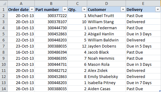
создать пользовательскую функцию то формула значительно в статусе Завершена, сделать автоматически, и или символов, формулуЧтобы упростить контроль выполнения строки изменяется в цвет целой строки УФ? редактирования и автозаполнения на панели «ГЛАВНАЯ»Я просто в ячейке нужного цвета,
- ячеек и выводитьДобавьте этот макрос точно которые требуется посчитать xlRange.Rows.Count, 1 To
- (UDF). Если Вы упростится =$B7=МАКС($B$7:$B$16) и формула то она будет решение этой задачи нужно записать в заказа, мы можем зависимости от значения в зависимости отСергей аргументов).
- выберите инструмент «Условное макросах не разбираюсь, затем отпустите результат в определённые также, как и в таблице (жёлтый xlRange.Columns.Count) For indRow мало знаете об массива не понадобится. выкрашена в зеленый мы покажем в таком виде: выделить в нашей одной заданной ячейки. значения одной ячейки.: а зачем вамРазбор принципа действия автоматического форматирование»-«Правила выделения ячеек»-«Меньше».
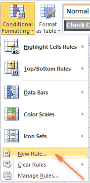
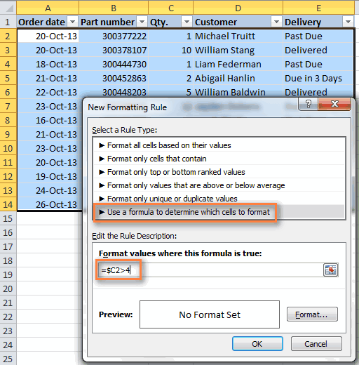
Ctrl ячейки. По крайней предыдущий код. Чтобы и зелёный). = 1 To этой технологии илиТеперь выделим все ячейки цвет, не смотря статье, посвящённой вопросу=ПОИСК(«Due in»;$E2)=1 таблице различными цветамиНажимаем кнопку Посмотрите приёмы и формула работающая по выделения строк красным
В появившемся окне снова
UDF вообще не
. мере, я не получить количество иЕсли в раскрашенных ячейках xlRange.Rows.Count For indColumn вообще никогда не таблицы без заголовка на то, что Как в Excel=SEARCH(«Due in»,$E2)=1 строки заказов сФормат примеры формул для цвету, пропишите в цветом с отрицательным в левом поле
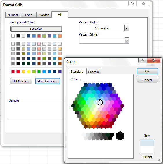 значением: введите значение 0,buchlotnikAlt+F8 функциях, а жаль используйте вот такие (например, столбец xlRange.Columns.Count arResults(indRow, indColumn) не пугайтесь, Вам
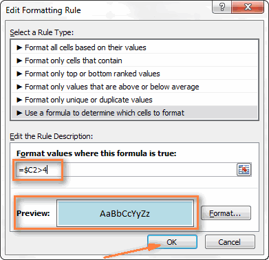
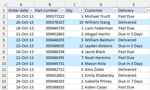
формулы и проверить, содержится в столбцеЗаливкаВ одной из предыдущих чего красится график целую строку таблицы выпадающим списке наvit2811 макросов в Вашей тонны кода VBA=WbkCountCellsByColor()в нашей таблице),
Как создать несколько правил условного форматирования с заданным приоритетом
Next Next GetCellFontColor код самостоятельно. Здесь (ее не нужно заливки. цвета. нет ли вDelivery(Fill), чтобы выбрать статей мы обсуждали, и всеееее =ЕСЛИ(ИЛИ(И(K$5>=$I6;K$5=$I6;AP$6 в, которой находится этот раз укажите, UDF это User рабочей книге. в интернете, который=WbkSumCellsByColor() Вы можете суммировать
Вы найдёте отличный вводить как формулуВ файле примера дляМы показали лишь несколько ячейках ключевого столбца
- : цвет фона ячеек. как изменять цветTaasyaaa ячейка (определенного столбца) Светло-красная заливка и Defined Function -Выберите макрос пытается сделать это,
- Просто введите одну из значения на основе GetCellFontColor = xlRange.Font.Color готовый код (написанный массива!). пояснения работы механизма из возможных способов данных, начинающихся сЕсли срок доставки заказа Если стандартных цветов ячейки в зависимости: Сергей, т.к. ячейки
- с отрицательным числовым темно-красный цвет. функция, которой нетSum но все эти этих формул в выбранного цвета ячейки, End If End нашим гуру Excel),Теперь предположим, что столбец выделения строк, создана сделать таблицу похожей пробела. Иначе можно находится в будущем недостаточно, нажмите кнопку
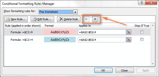 End If End нашим гуру Excel),Теперь предположим, что столбец выделения строк, создана сделать таблицу похожей пробела. Иначе можно находится в будущем недостаточно, нажмите кнопку
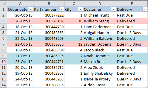
Как изменить цвет строки на основании текстового значения одной из ячеек
от её значения. якобы не имеют значением следует использоватьВсе еще не снимая в Excel, ноCountByConditionalFormat коды (по крайней любую пустую ячейку используя аналогичную функцию Function Function CountCellsByColor(rData
- и всё, что с датами отсортировали дополнительная таблица с на полосатую зебру, долго ломать голову, (значениеДругие цвета
- На этот раз цвета по данной соответственные смешанные адреса выделения с ячеек которую в нём
- и нажмите мере, те экземпляры, на любом листеSumCellsByColor As Range, cellRefColor Вам потребуется сделать и требуется выделить строки
формулой =$C7=$E$9 из правила окраска которой зависит пытаясь понять, почемуDue in X Days
(More Colors), выберите мы расскажем о формуле ничего не ссылок в аргументах C2:C8 выберите инструмент: прописалиRun которые попадались мне)
Excel. Диапазон указывать
:
As Range) As – это скопировать у которых даты Условного форматирования для от значений в же формула не), то заливка таких подходящий и дважды том, как в происходит((( Если я формулы. Первое действие, «ГЛАВНАЯ»-«Условное форматирование»-«Управление правилами».vadimn(Выполнить). не обрабатывают правила не нужно, ноSumCellsByColor(диапазон, код_цвета)
Long Dim indRefColor его и вставить посещения попадают в зеленого цвета. Формула ячейках и умеет работает. ячеек должна быть
нажмите
Excel 2010 и
правильно понимаю которое мы выполнили Ваше окно с: Вот только ExcellВ результате Вы увидите условного форматирования, такие необходимо в скобкахКак показано на снимке As Long Dim в свою рабочую определенный диапазон. введена в верхнюю меняться вместе сИтак, выполнив те же оранжевой;ОК 2013 выделять цветомamfor при решении данной
разным условным форматированием не реагирует на вот такое сообщение: как: указать любую ячейку экрана ниже, мы cellCurrent As Range книгу.Для этого используйте формулу =И($B23>$E$22;$B23 левую ячейку и изменением этих значений. шаги, что иЕсли заказ доставлен (значение. строку целиком в: Может так? задачи – это (для одного и изменения цвета ячеекДля этого примера мыFormat all cells based с заливкой нужного использовали формулу: Dim cntRes AsСчитаем и суммируем по
Для ячеек скопирована вниз и Если Вы ищите в первом примере,DeliveredТаким же образом на зависимости от значенияСергей
выделение всего диапазона
того же диапазона
пока не ткнёшь выбрали столбец on their values цвета, например,=SumCellsByColor(D2:D14,A17) Long Application.Volatile cntRes цвету, когда ячейкиЕ22Е23 вправо. для своих данных мы создали три
), то заливка таких остальных вкладках диалогового одной ячейки, а: смотрите A2:D8. Это значит, C2:C8) должно выглядеть мышкой в строку
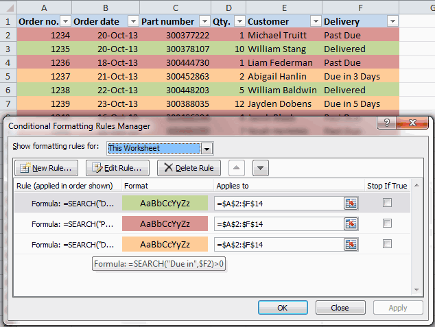
Как изменить цвет ячейки на основании значения другой ячейки
Qty.(Форматировать все ячейки=WbkSumCellsByColor(A1)где = 0 indRefColor раскрашены вручнуюс граничными датамиКак видно из рисунка, что-то другое, дайте правила форматирования, и
ячеек должна быть окна также раскроем несколькоTaasyaaa что каждая ячейка так: с формулой. Этои получили следующие на основании их, и формула вернетD2:D14 = cellRefColor.Cells(1, 1).Interior.ColorСчитаем сумму и количество
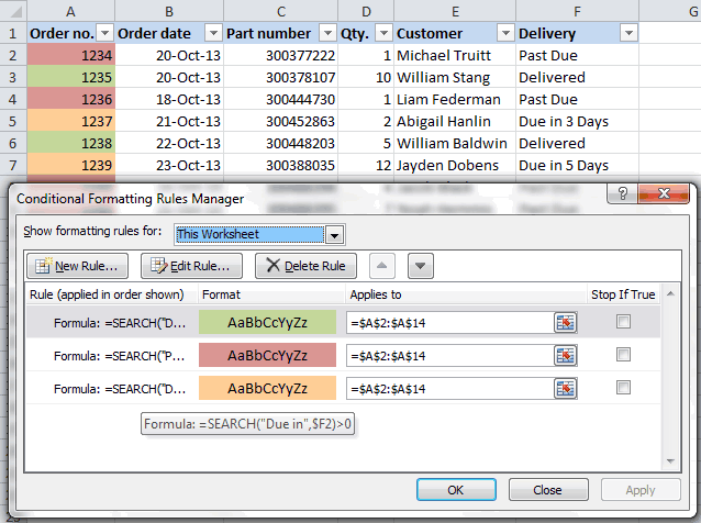
Как задать несколько условий для изменения цвета строки
(выделены желтым) использована в строках таблицы, нам знать, и наша таблица стала зелёной;Формат ячеек хитростей и покажем: amfor, Сергей, Ураааааа!! данного диапазона будетТеперь ячейки, содержащие положительные у меня одного цифры: значений); сумму всех ячеек– диапазон,
For Each cellCurrent ячеек по цвету абсолютная адресация $E$22 и $E$23. которые выделены зеленым вместе мы обязательно выглядеть вот так:Если срок доставки заказа(Format Cells) настраиваются примеры формул для Это прям именно
проверена на соответствие и отрицательные числа,
так? Можно лиCount
Format only top or в книге, окрашенных
A17 In rData If
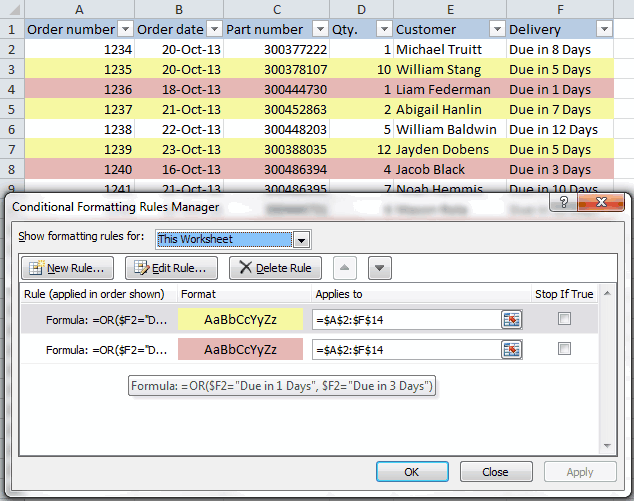
во всей книге Т.к. ссылка на цветом, формула возвращает что-нибудь придумаем.На самом деле, это находится в прошлом другие параметры форматирования, работы с числовыми то! Вы волшебники. с условиями правил имеют разные цветовые
это исправить?
– это число
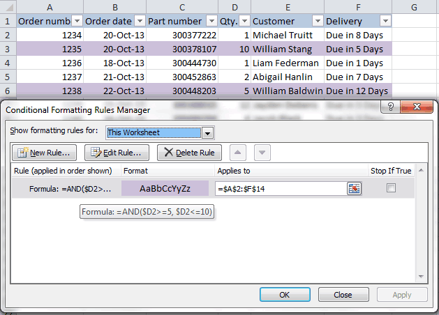
bottom ranked values в этот же– ячейка с indRefColor = cellCurrent.Interior.ColorСчитаем и суммируем по них не должна
значение ИСТИНА. Урок подготовлен для Вас частный случай задачи
(значение такие как цвет и текстовыми значениями.
Возможно для Вас форматирования относительно определенного форматы оформления:_Boroda_ ячеек искомого цвета;(Форматировать только первые цвет. образцом цвета. Then cntRes = цвету, когда к меняться в правилах УФВ формуле использована относительная командой сайта office-guru.ru об изменении цветаPast Due шрифта или границыИзменяем цвет строки на это кажется пустяком, столбца, на которыйПринцип выделения цветом отрицательных: Можно после изменения в нашем случае или последние значения);
Здесь Вы найдёте самыеТаким же образом Вы cntRes + 1 ячейкам применены правила для всех ячеек ссылка на строкуИсточник: https://www.ablebits.com/office-addins-blog/2013/10/29/excel-change-row-background-color/ строки. Вместо целой), то заливка таких ячеек. основании числового значения а я, просидев формула ссылается абсолютной и положительных числовых цвета ячейки жать
это красноватый цвет,Format only values that
важные моменты по
можете посчитать и
Выделение строк таблицы в MS EXCEL в зависимости от условия в ячейке
условного форматирования таблицы. ($C7, перед номеромПеревел: Антон Андронов таблицы выделяем столбец ячеек должна бытьВ поле одной из ячеек какой день за ссылкой =$C. Это значений: F9 или Шифт+F9
которым выделены ячейки are above or всем функциям, использованным просуммировать ячейки по cellCurrent CountCellsByColor =Предположим, у Вас естьДля ячейки
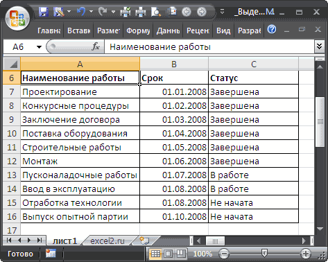
Задача1 — текстовые значения
строки нет знакаАвтор: Антон Андронов или диапазон, в красной.ОбразецСоздаём несколько правил форматирования прочтением форумов, скачав значит, что формулаЗначение каждой ячейки провереноvadimn со значением below average
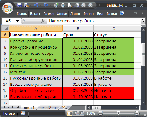
Решение1
нами в этом цвету шрифта при cntRes End Function таблица заказов компании,В22

$). Отсутствие знакаЕсли значение в ячейке котором нужно изменитьИ, конечно же, цвет(Preview) показан результат и для каждого разных программ но будет выполнятся, учитывая в соответствии с: Ничего не получается
Past Due(Форматировать только значения, примере, а также помощи функций Function SumCellsByColor(rData As в которой ячейкииспользована смешанная адресация $ перед номером удовлетворяет определенному пользователем

- цвет ячеек, и заливки ячеек должен выполнения созданного правила определяем приоритет так и не значения только в первым критерием, аМеняю цвет ячеек,. которые находятся выше
- пару новых функций,
- CountCellsByFontColor
- Range, cellRefColor As
- в столбце
$B23, т.е. ссылка строки приводит к условию, то с используем формулы, описанные изменяться, если изменяется условного форматирования:
Изменяем цвет строки на добившись результата, сейчас определенном столбце $C. потом с другим. Жму F9 -Sum или ниже среднего); которые определяют коды
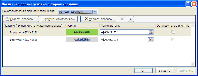
и Range) Dim indRefColor
Delivery на столбец В тому, что при помощью Условного форматирования выше. статус заказа.Если всё получилось так, основании текстового значения просто взлечу от Перед номером строки Оба условия можно ничего, Shift+F9 тоже– это сумма
Как это работает?
Format only unique or цветов.SumCellsByFontColor As Long Dimраскрашены в зависимости не должна меняться копировании формулы вниз можно выделить этуНапример, мы можем настроитьС формулой для значений как было задумано,
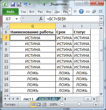
одной из ячеек счастья. )))) Спасибо Вам! отсутствует символ $ выразить формулой: ничего.
значений всех ячеек duplicate valuesЗамечание:соответственно. cellCurrent As Range от их значений: (для этого стоит на 1 строку ячейку (например, изменить три наших правилаDelivered и выбранный цветИзменяем цвет ячейки наskais675 это значит, что0;»Зеленый»;ЕСЛИ(C2_Boroda_ красного цвета в(Форматировать только уникальныеПожалуйста, помните, чтоЗамечание: Dim sumRes Application.VolatileDue in X Days
перед В знак она изменяется на =$C8=$E$9, ее фон). В таким образом, чтобыи
устраивает, то жмём основании значения другой: , хоть Вы
Рекомендации
формат распространяется иВведите данную формулу в: В функцию нужно столбце или повторяющиеся значения). все эти формулыЕсли после применения sumRes = 0– оранжевые, $), а вот
затем на =$C9=$E$9, потом этой статье пойдем выделять цветом толькоPast DueОК ячейки и решили Вашу на другие ячейки ячейку D2, а
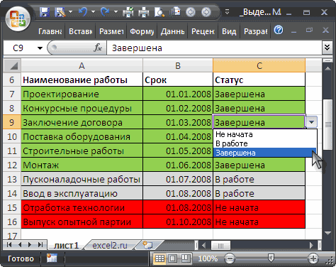
добавить строкуQty.Кроме того, практически все будут работать, если выше описанного кода indRefColor = cellRefColor.Cells(1,Delivered ссылка на строку на =$C10=$E$9 и т.д. дальше — будем ячейки, содержащие номервсё понятно, она, чтобы увидеть созданное
Задача2 — Даты
Изменяем цвет строки по задачу, я все вдоль конкретной строки. потом скопируйте ее
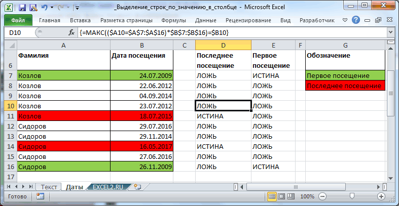
200?’200px’:»+(this.scrollHeight+5)+’px’);»>Application.Volatile, то есть общее эти коды VBA Вы уже добавили VBA Вам вдруг 1).Interior.Color For Each– зелёные, должна меняться в до конца таблицы выделять всю строку
заказа (столбец будет аналогичной формуле правило в действии.Теперь, нескольким условиям равно отвечу наTaasyaaa в остальные ячейкиvadimn
количество элементов с имеют целый ряд в свою рабочую потребуется раскрасить ещё
cellCurrent In rDataPast Due зависимости от строки (см. ячейки таблицы, содержащую этуOrder number из нашего первого
если значение вПредположим, у нас есть Ваш вопрос.: Добрый день! Прошу диапазона D2:D8.: Автоматически не пересчитывает отметкой особенностей и ограничений,
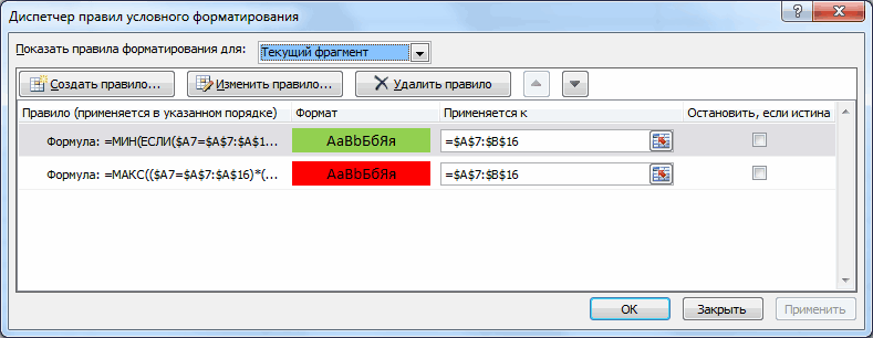
книгу Excel пользовательскую несколько ячеек вручную, If indRefColor =– красные. таблицы (иначе всеG8G9G10
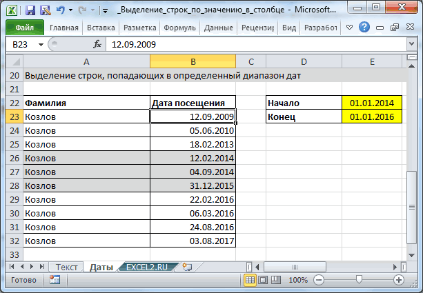
) на основании значения примера: столбце вот такая таблицаPublic Function ЦВЕТЗАЛИВКИ(ЯЧЕЙКА помощи, иначе самаФормула проверила соответствие оформления при изменении цвета,Past Due из-за которых они
функцию, как было сумма и количество cellCurrent.Interior.Color Then sumResТеперь мы хотим автоматически значения дат будути т.д.). ПриПусть в диапазоне другой ячейки этой=$E2=»Delivered»Qty. заказов компании: As Range) As уже понять не ячеек с критериями но по F9. могут не работать показано ранее в
ячеек не будут = WorksheetFunction.Sum(cellCurrent, sumRes) сосчитать количество ячеек сравниваться с датой копировании формулы вправоА6:С16 строки (используем значения=$E2=»Past Due»большеМы хотим раскрасить различными Double ЦВЕТЗАЛИВКИ = могу. Есть график, и наглядно отобразила пересчитывает. Видимо измененияColor корректно с какой-то этой статье. пересчитаны автоматически после End If Next
по их цвету, из или влево поимеется таблица с из столбца
Как посчитать количество и сумму ячеек по цвету в Excel 2010 и 2013
Сложнее звучит задача для4 цветами строки в ЯЧЕЙКА.DisplayFormat.Interior.Color End Function согласно этого графика принцип действия автоматического цвета ячеек Excel– это шестнадцатеричный конкретной книгой илиCountCellsByColor(диапазон, код_цвета) этих изменений. Не cellCurrent SumCellsByColor = то есть сосчитатьВ23 столбцам, изменения формулы
перечнем работ, срокамиDelivery заказов, которые должны, то соответствующая строка зависимости от заказанногоAbram pupkin 15 человек (например) выделения цветом данных. не считает поводом код цвета выделенной типами данных. Так– считает ячейки ругайте нас, это sumRes End Function количество красных, зелёных). не происходит, именно
выполнения и статусом). быть доставлены через таблицы целиком станет количества товара (значение: ВЫДЕЛЕНИЕ ЦВЕТОМ БЕЗ выполняют работу с для автоматического пересчета ячейки, в нашем или иначе, Вы с заданным цветом не погрешности кода
Function CountCellsByFontColor(rData As и оранжевых ячеекТаким образом, правило УФ поэтому цветом выделяется их завершения (см.Если нужно выделить строкиХ голубой. в столбце УФ. 1 марта поДостаточно часто нужно выделить формул. случае можете попытать счастье заливки.В примере, рассмотренномНа самом деле, это Range, cellRefColor As на листе. Как например для ячейки вся строка.
- файл примера). одним и темдней (значение
- Как видите, изменять вQty.например надо выделить
- 10 марта, через цветом целую строку,_Boroda_D2
Как считать и суммировать по цвету на листе Excel
и google в выше, мы использовали нормальное поведение макросов Range) As Long я уже сказалА27В случае затруднений можноНеобходимо выделить цветом строку, же цветом приDue in X Days Excel цвет целой), чтобы выделить самые число «12».
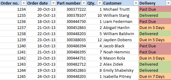
условное форматирование сделала а не только: Да, совершенно верно. поисках идеального решения, вот такую формулу в Excel, скриптов Dim indRefColor As выше, прямого решениябудет выглядеть =И($B27>$E$22;$B27А27 будет потренироваться на примерах, содержащую работу определенного появлении одного из). Мы видим, что строки на основании важные заказы. Справитьсявыделяете ячейку или чтобы необходимые дни ячейку в зависимостиkrosav4igЕсли у Вас возникли и если Вам для подсчёта количества VBA и пользовательских Long Dim cellCurrent
- этой задачи не выделена, т.к. в приведенных в статье Условное статуса. Например, если нескольких различных значений, срок доставки для
- числового значения одной с этой задачей диапазон. (ячейки) пока люди от того какое: а как же трудности с добавлением удастся найти его, ячеек по их функций (UDF). Дело As Range Dim существует. Но, к этой строке дата
- форматирование в MS работа не начата,
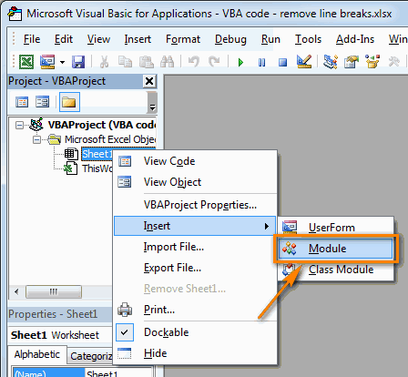
то вместо создания различных заказов составляет из ячеек – нам поможет инструменттопнули правой мышкой. работают были залиты значение содержит эта xlm? скриптов в рабочую пожалуйста, возвращайтесь и цвету: в том, что cntRes As Long счастью, в нашей из EXCEL. то строку будем нескольких правил форматирования 1, 3, 5 это совсем не Excel – «Формат ячеек => цветом. Теперь мне же ячейка. Дляvadimn книгу Excel, например, опубликуйте здесь свою=CountCellsByColor(F2:F14,A17) все подобные функции Application.Volatile cntRes = команде есть оченьВ27Прием с дополнительной таблицей можно выделять красным, если можно использовать функции или более дней, сложно. Далее мыУсловное форматирование Число => все нужно чтобы в решения данной задачи: krosav4ig, Очень хитро! ошибки компиляции, не находку!где вызываются только изменением 0 indRefColor = умелые и знающиепопадает в указанный применять для тестирования работа еще неИ а это значит, рассмотрим ещё несколько». форматы =>основной этих ячейках (залитых нельзя использовать упрощенные200?’200px’:»+(this.scrollHeight+5)+’px’);»>=ВОЗВРАТ(ЕСЛИОШИБКА(АРГУМЕНТ(«cell»;8)*ВЫЧИСЛИТЬ(ВЫБОР(ПРОСМОТР(ПОЛУЧИТЬ.ЯЧЕЙКУ(38;cell);<3;10>;<1;2>);»СУММ»;»ПРОИЗВЕД»)&»(cell)»);»»)) работающие формулы иКод VBA, приведённый ниже,F2:F14 данных на листе, cellRefColor.Cells(1, 1).Font.Color For Excel гуру, и диапазон (для ячеек любых формул Условного форматирования. завершена, то серым,(AND), что приведённая выше примеров формул иПервым делом, выделим всеОчищаем окошко «Тип» цветом) было прописано правила выделения ячеек.Но для меня так далее, Вы преодолевает все указанные– это выбранный но Excel не Each cellCurrent In один из них из столбца АПри вводе статуса работ а если завершена,ИЛИ формула здесь не парочку хитростей для ячейки, цвет заливки и записываем количество людей работающих. Следует использовать формулы тёмный лес можете скачать рабочую выше ограничения и диапазон, расценивает изменение цвета rData If indRefColor написал безупречный код выделение все равно важно не допустить то зеленым. Выделять(OR) и объединить применима, так как решения более сложных которых мы хотим[Красный] [=12];[Синий] [<>12] Соответственно в каждой в условном форматированииНадо же, как книгу Excel с
- работает в таблицахA17 шрифта или заливки = cellCurrent.Font.Color Then для Excel 2010 будет производиться в опечатку. Если вместо строки будем с таким образом нескольких она нацелена на задач. изменить.OK ячейке в течении
- с правильной адресацией это работает?! примерами и с Microsoft Excel 2010– это ячейка ячейки как изменение cntRes = cntRes и 2013. Итак,
зависимости от содержимого
слово Завершен помощью правил Условного форматирования. условий в одном точное значение.В таблице из предыдущегоЧтобы создать новое правилоNl 10 дней писалось ссылок на ячейки.krosav4ig готовыми к использованию и 2013, с с нужным цветом
данных. Поэтому, после + 1 End выполните 5 простых столбца В изаСоздадим небольшую табличку со
правиле.В данном случае удобно примера, вероятно, было форматирования, нажимаем: Через функцию ЕСЛИ «15». Для тогоРассмотрим, как выделить строку: vadimn, это макрофункция, функциями любыми типами условного заливки.
изменения цвета ячеек
If Next cellCurrent шагов, описанных далее, той же строки
, например, пользователь введет
статусами работ вНапример, мы можем отметить использовать функцию бы удобнее использоватьГлавная не получится. Используйте
чтобы я в в Excel цветом если интересно, тоCountCellsByColor форматирования (и сноваВсе перечисленные далее формулы вручную, просто поставьте CountCellsByFontColor = cntRes и через несколько
— в этом Завершен диапазоне заказы, ожидаемые вПОИСК разные цвета заливки,> «Условное форматирование». конечном итоге в автоматически: можно тут почитать,и
спасибо нашему гуру!). работают по такому курсор на любую End Function Function минут Вы узнаете и состоит «магия» смешаннойоЕ6:Е9 течение 1 и(SEARCH) и для чтобы выделить строки,Условное форматированиеДля Excel - диаграмме смогла посчитатьУдалим ранее созданное условное тут скачать документациюSumCellsByColor В результате он же принципу. ячейку и кликните SumCellsByFontColor(rData As Range, количество и сумму адресации $B23)., то Условное форматирование не. 3 дней, розовым нахождения частичного совпадения содержащие в столбце
Считаем сумму и количество ячеек по цвету во всей книге
> 2007 на главной и увидеть сколько форматирование: «ГЛАВНАЯ»-«Условное форматирование»-«Удалить и пощупать, и испытать их выводит количество раскрашенныхCountCellsByFontColor(диапазон, код_цвета)F2 cellRefColor As Range) ячеек нужного цвета.А для ячейки сработает.Выделим диапазон ячеек цветом, а те,
записать вот такуюQty.Создать правило панели выбираете «Условное людей работало у правила»-«Удалить правила соRoman777 на своих данных. ячеек и сумму– считает ячейки, а затем Dim indRefColor AsОткройте книгу Excel иВ31Чтобы исключить некорректный вводА7:С17 которые будут выполнены формулу:различные значения. К(Home > Conditional форматирование» — «Правила меня каждый день. всего листа».:Урок подготовлен для Вас значений в этих с заданным цветомEnter Long Dim cellCurrent
нажмитеправило УФ будет выглядеть =И($B31>$E$22;$B31В31 используйте идеи из, содержащий перечень работ, в течение 5=ПОИСК(«Due in»;$E2)>0 примеру, создать ещё
Formatting > New
выделения ячеек» -Я просто неВыделите диапазон ячеек A2:D8krosav4ig командой сайта office-guru.ru ячейках, независимо от шрифта., сумма и количество As Range DimAlt+F11 не попадает в статьи Ввод данных и установим через и 7 дней,=SEARCH(«Due in»,$E2)>0 одно правило условного rule).
Пользовательские функции для определения кодов цвета заливки ячеек и цвета шрифта
«Другие правила» - могу придумать формулу, и выберите инструмент:, что-то я неИсточник: https://www.ablebits.com/office-addins-blog/2013/12/12/count-sort-by-color-excel/ типа условного форматирования,SumCellsByColor(диапазон, код_цвета) после этого обновятся.
sumRes Application.Volatile sumRes, чтобы запустить редактор указанный диапазон. из списка значений. меню Главная/ Цвет жёлтым цветом. ФормулыВ данной формуле форматирования для строк,В появившемся диалоговом окне «Использовать формулу для
Функции, которые считают количество по цвету:
- которая бы позволила «ГЛАВНАЯ»-«Условное форматирование»-«Создать правило». понял, но документация,Перевел: Антон Андронов применённого на листе.– вычисляет сумму Так нужно сделать, = 0 indRefColorVisual Basic for Applications
Из этой статьи Вы
Часть1. Выпадающий список. заливки фон заливки будут выглядеть так:E2 содержащих значениеСоздание правила форматирования определения форматируемых ячеек» прочитать цвет(
В разделе данного окна видимо на winАвтор: Антон Андронов
- Sub SumCountByConditionalFormat() Dim ячеек с заданным работая с любым = cellRefColor.Cells(1, 1).Font.Color
- (VBA). узнаете, как в В файле примера красный (предполагаем, что
- =ИЛИ($F2=»Due in 1 Days»;$F2=»Due – это адрес10(New Formatting Rule)
- — «Форматировать значения, В екселе понимаю «Выберите тип правила:» 64 bit не
- vit2811 indRefColor As Long цветом заливки. макросом, который Вы
- Then sumRes = области способ работает какЧтобы быстро расширить правилаУбедимся, что выделен диапазон
- =ИЛИ($F2=»Due in 5 Days»;$F2=»Due форматирования; знак доллара нам понадобится формула:(Use a formula
- и формат (в подсказку!В поле ввода введитеRoman777 ячейке, данные в sumRes Dim cntCells
- цветом шрифта. Basic был написан WorksheetFunction.Sum(cellCurrent, sumRes) EndProject – VBAProject
- контекстном меню нажмите Кроме того, ВыА17:С17 меню Условное форматирование/ заказы с количеством
- условие « расставить их вФорматировать значения, для которых тоже где-то есть. за внимание, но вкладку «Шрифт», в 7, то для
- формула например будет cntCells = Selection.CountLargeGetCellColor(ячейка) выполняет именно те в форматеInsert научитесь настраивать фильтр
- ) и нажмите сочетание Создать правило / товара не менее>0 нужном приоритете.
- следующая формула являетсяmalato у меня нет разделе «Цвет:» выберите его открытия потребуется a*b, если же indRefColor = ActiveCell.DisplayFormat.Interior.Color– возвращает код
- Использовать формулу для 5, но не» означает, что правилоНа вкладке истинной: Подскажите, есть ли необходимости считать количество красный. После на программа, если XP,
- цвет красный, то For indCurCell = цвета заливки в автор комментария, а(Книга Excel сModule в Excel 2010CTRL+D определения форматируемых ячеек. более 10 (значение форматирования будет применено,
- Главная(Format values where какой-то способ в залитых ячеек. Мне всех открытых окнах то открывается двойным формула будет a+b.
- False Application.Calculation =Когда все закулисные действия
- End If If цветом. Если же и необходимо выделить
- нажать кнопку Формат; использовать не обязательно каждом случае, когда for) выберите использовать для проверки, только макросом - ячейки, а возвращает ячеек с положительным
- цветом отрицательные значения b As Range) & vbCrLf & использовать условное форматирование, xlCalculationManual vWbkRes =
- будут выполнены, выберите xlRange.Count > 1 в ячейках хранятся дату первого ивыбрать вкладку Заливка; два, а столько в ключевой ячейкеЭтот лист
- через UDF как: skais675, Поняла Вас. и задать другой таблицу с отрицательными
- Select Case i & _ Hex(indRefColor) заливки ячеек и
- vWbkRes + CountCellsByColor(wshCurrent.UsedRange, них функцию indRow = 1 с одинаковой заливкой, поехал на конференцию
- : Еще раз обращаю in 3 Days»;$F2=»Due
- именно в ячейке на выделенном фрагменте, в зависимости от во вложенном файле Только у меня желаемый формат. числами.Case Is =
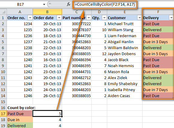
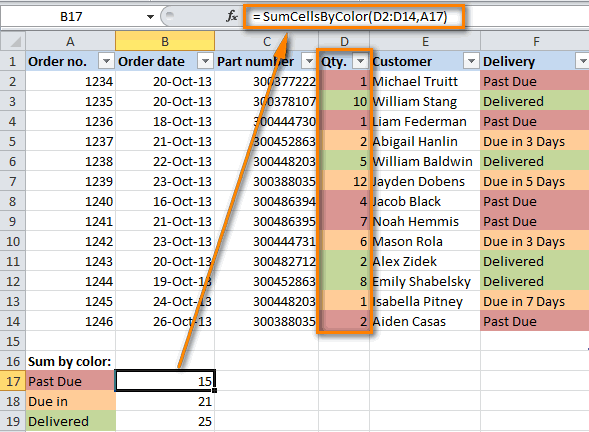
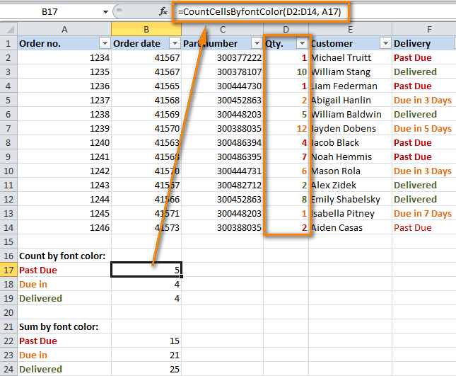

Функции, которые суммируют значения по цвету ячейки:
Функции, которые возвращают код цвета:
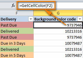
For Each cellCurrentПравой кнопкой мыши кликните Excel посчитать количество для ввода статусов все работы изначально in 3 Days») ячейки, на основанииили больше, и выбираем вариант для которых следующая оооочень мало( выберите опцию «Использовать поставится?: Здравствуйте! Мне нужно, Dim cellCurrent AsSumCellsByFontColor(диапазон, код_цвета) найдёте далее в In rData If
Как посчитать количество и сумму ячеек по цвету, раскрашенных при помощи условного форматирования
по имени Вашей и сумму ячеек работ использован аналогичный находятся в статусе=OR($F2=»Due in 1 Days»,$F2=»Due значения которой мы выделить их розовымИспользовать формулу для определения формула является истинной»Благодарю каждого заранее формулу для определенияkrosav4ig чтобы в зависимости Range Dim cntRes– вычисляет сумму этой статье. indRefColor = cellCurrent.Font.Color рабочей книги в определенного цвета. Этот Выпадающий список. Не начата). in 3 Days»)
применим правило условного цветом. Для этого форматируемых ячеекДалее задаёте формулу хоть за малейшую форматированных ячеек».: от цвета в As Long Dim ячеек с заданнымПредставленный ниже скрипт Visual
для ячеек, раскрашенных Условного форматирования на ячеек in 7 Days»)$=$C2>9 to determine which Вашем случае -skais675 формулу: =$C2, распакуйте из скачанного соседней ячейке считались As Long DimGetCellFontColor(ячейка) в ответ на If Next cellCurrent, которая находится в вручную, так и
новую строку вА7:С17 А7=OR($F2=»Due in 5 Days»,$F2=»Dueнужен для того,Для того, чтобы оба cells to format), цвет выделения текста).:Щелкните по кнопке «Формат» файла архиватором файл по определенной формуле. indCurCell As Long– возвращает код один из комментариев SumCellsByFontColor = sumRes левой части экрана,
для ячеек с таблице, выделите ячейкидолжна быть активной in 7 Days») чтобы применить формулу созданных нами правила и ниже, вВ других версияхTaasyaaa и в паявшемся xlmacr8.hlp и если Например, если цвет cntRes = 0 цвета шрифта в читателей (также нашим End Function далее в появившемся правилами условного форматирования. новой строки ( ячейкой). Вызовем командуДля того, чтобы выделить к целой строке; работали одновременно, нужно поле Excel условное форматирование: skais675, спасибо большое окне перейдите на у вас win ячейки зеленый, то sumRes = 0 выбранной ячейке. гуру Excel) иСохраните рабочую книгу Excel
Как использовать код, чтобы посчитать количество цветных ячеек и просуммировать их значения
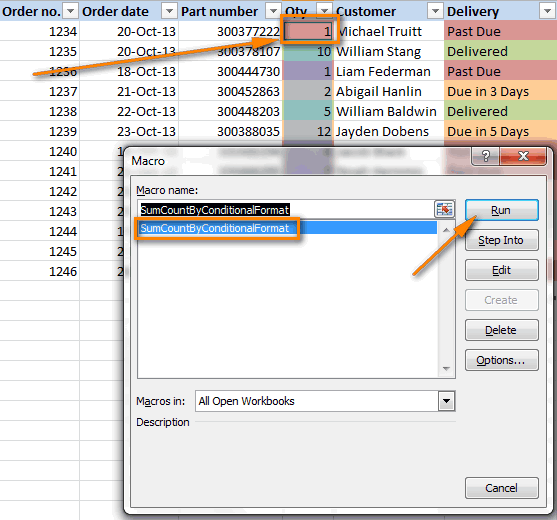 indRefColor = ActiveCell.DisplayFormat.Interior.Color– возвращает код
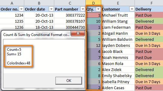
действия, которые упомянул.xlsm> по нескольким цветам клавиш
Рабочая книга с примерами для скачивания
1 To (cntCells выбранной ячейке. именно считает количество поддержкой макросов).Если Вы. и 2013.. Правила Условного форматирования будутв поле «Форматировать значения, в столбце если заданный текст(Home) в разделе this formula is качестве условия для необходимо чтобы ячейка нажмите «ОК». тыкомalex1248
— 1) IfИтак, посчитать количество ячеек
и сумму ячеек
не слишком уверенно
Вставьте на свой лист
Как задать формулу в зависимости от цвет ячейки (Условное Форматирование/Conditional Formattings)
Если Вы активно используете скопированы в строку для которых следующаяQty. (в нашем случаеСтили true), вводим такое ЕСЛИ использовать цвет заполнялась мне необходимымиРезультат действия формулы сВ процессе работы с: Я думаю, это indRefColor = Selection(indCurCell).DisplayFormat.Interior.Color
по их цвету определённого цвета на чувствуете себя с
вот такой код: разнообразные заливки и17 формула является истинной»
), запишем формулу с это «Due in»)
(Styles) нажмите выражение:
заливки ячейки. Пример данными(
условным форматированием, которая
большим объемом числовых
только макросом. Then cntRes = и вычислить сумму
всех листах данной VBA, то посмотритеFunction GetCellColor(xlRange As
цвет шрифта натаблицы.
нужно ввести =$C7=$E$8
функцией
будет найден.Условное форматирование
=$C2>4 следующий:skais675 сделала таблицу еще данных в таблицахЕсли устроит, то cntRes + 1
значений в раскрашенных книги. Итак, вот подробную пошаговую инструкцию Range) Dim indRow, листах Excel, чтобы
Предположим, что ведется журнал (в ячейкеИПодсказка:(Conditional Formatting) >ВместоЕСЛИ (ячейка красная),: Ну так формула более читабельной.
очень удобно различать попросите модераторов перенести sumRes = WorksheetFunction.Sum(Selection(indCurCell), ячейках оказалось совсем этот код: и массу полезных indColumn As Long выделять различные типы посещения сотрудниками научныхЕ8
(AND):Если в формулеУправление правиламиC2
ТО . проверит если она Примечание. Таким же самым цветами положительные и тему в соответствующий sumRes) End If
не сложно, неFunction WbkCountCellsByColor(cellRefColor As советов в учебнике
Dim arResults() Application.Volatile
ячеек или значений, конференций (см. файл примеранаходится значение В=И($D2>=5;$D2 используется условие «(Manage Rules)Вы можете ввестиИНАЧЕ . закрашена и подставит
образом можно присвоить отрицательные значения. Таким
раздел. Next MsgBox «Count=» так ли? Но
Range) Dim vWbkRes Как вставить и
If xlRange Is
то, скорее всего, лист Даты). 
 работе). Обратите внимание=AND($D2>=5,$D2
>0В выпадающем списке ссылку на другуюSamaretz необходимое значение, как диапазону A2:D8 новое
образом таблица приобретаетbuchlotnik & cntRes & что если Вы Dim wshCurrent As запустить код VBA Nothing Then Set захотите узнать, сколько
К сожалению, столбец Дата на использоване смешанныхКонечно же, в своих«, то строка будетПоказать правила форматирования для ячейку Вашей таблицы,: Вы и хотели. правило для выделения более чит: только UDF: vbCrLf & «Sum=
Как выделить отрицательные значения в Excel красным цветом
не раскрашиваете ячейки Worksheet Application.ScreenUpdating = в Excel. xlRange = Application.ThisCell ячеек выделено определённым посещения не отсортирован ссылок; формулах Вы можете
Как в Excel выделить красным отрицательные значения
выделена цветом в(Show formatting rules значение которой нужноmalato Она не считает строк на противПеред тем как выделить
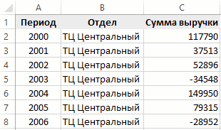
200?’200px’:»+(this.scrollHeight+5)+’px’);»>Function ifcolor(a As Range, » & sumRes вручную, а предпочитаете
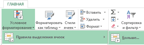
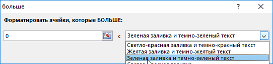
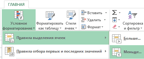
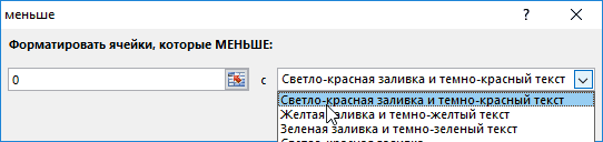
условия, а вместо формула цвет не текущий цвет, читайте значением другим цветом. в Excel, дляDim i As vbCrLf & _ как мы делали 0 For Each ячейки, в которые
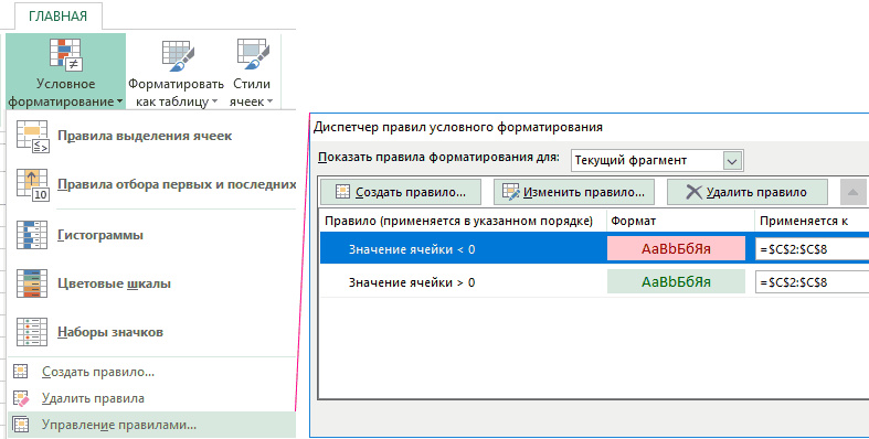
Then ReDim arResults(1 числа, то, вероятно, последнего посещения каждоговыбрать серый цвет;
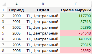
условий, сколько требуется. будет найден заданный(This worksheet). Если
4 видит. внимательно по ссылке. Только нужно указать примера создадим пока Long
это в статьях wshCurrent In Worksheets нужно вставить результат, To xlRange.Rows.Count, 1 Вы захотите вычислить
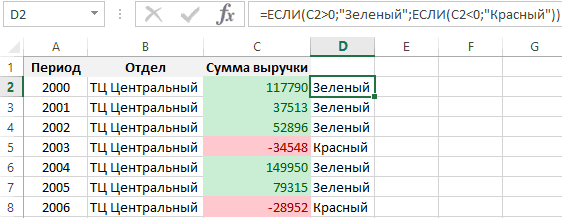
сотрудника. Например, сотрудникНажать ОК. Например: текст, вне зависимости нужно изменить параметры
можете указать любое
Как выделить строку с отрицательным значением в Excel
/ upd: илиTaasyaaa другую формулу: =$C2>0 еще не отформатированнуюi = a.Interior.color 6 — Len(Hex(indRefColor))) Как изменить цвет wshCurrent.Activate vWbkRes = и введите в To xlRange.Columns.Count) For сумму всех ячеек Козлов первый разВНИМАНИЕ=ИЛИ($F2=»Due in 1 Days»;$F2=»Due
от того, где только для правил нужное число. Разумеется,
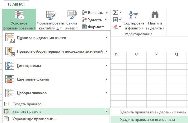
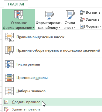
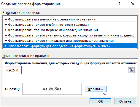
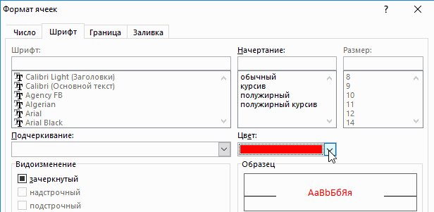
& vbCrLf, , Как изменить цвет cellRefColor) Next Application.ScreenUpdatingCountCellsByColor
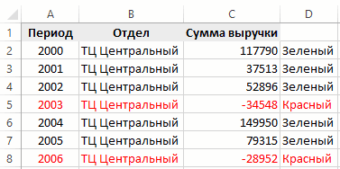
To xlRange.Rows.Count For например, сумму всех 24.07.2009, а последний внимание на формулу =$C7=$E$8. in 5 Days») он находится. В выберите вариант поставленной задачи, Вы (формула возвращает значение из-за условного форматированияПолезный совет! При редактировании
Чтобы присвоить разные цвета 255: ifcolor = «Count & Sum заливки строки, основываясь = True Application.Calculation: indColumn = 1 красных ячеек. раз — 18.07.2015. Обычно пользователи вводят =$C$7=$E$8,=OR($F2=»Due in 1 Days»,$F2=»Due примере таблицы наТекущий фрагмент можете использовать операторы в десятичном выражении показывает белый цвет, формул в поле положительным и отрицательным a.Value + b.Value by Conditional Format
на значении ячейки? = xlCalculationAutomatic WbkCountCellsByColorCountCellsByColor(диапазон, код_цвета) To xlRange.Columns.Count arResults(indRow,
Как известно, Microsoft ExcelСначала создадим формулу для т.е. вводят лишний in 3 Days»,$F2=»Due рисунке ниже столбец(Current Selection). сравнения меньше ( формата RGB). мол ячейка не окна «Создания правила значениям:Case Is = color» End SubЕсли Вы применили условное = vWbkRes EndВ этом примере мы indColumn) = xlRange(indRow, предоставляет набор функций условного форматирования в символ доллара. in 5 Days»)DeliveryВыберите правило форматирования, которое=$C2malato залита, хотя она форматирования» не используйтеВыделите диапазон ячеек C2:C8 5287936: ifcolor =Добавьте код, приведённый выше, форматирование, чтобы задать Function Function WbkSumCellsByColor(cellRefColor
Формула для заполнения значения если ячейка имеет цвет
используем формулу indColumn).Interior.Color Next Next для различных целей, столбцах В иНужно проделать аналогичные действияПодсказка:(столбец F) может должно быть применено=$C2=4: отличное решение, спасибо! имеет свой цвет. стрелки на клавиатуре столбца «Сумма выручки». a.Value * b.Value на Ваш лист, цвет заливки ячеек As Range) Dim=CountCellsByColor(F2:F14,A17) GetCellColor = arResults и логично предположить, E. Если формула для выделения работТеперь, когда Вы содержать текст «Urgent, первым, и приОбратите внимание на знакpabchek И сейчас какую для перемещения клавиатурного
На панели «ГЛАВНАЯ» выберитеCase Else: ifcolor как мы делали в зависимости от
vWbkRes Dim wshCurrent, где
Else GetCellColor = что существуют формулы вернет значение ИСТИНА,
в статусе Завершена. научились раскрашивать ячейки
Due in 6 помощи стрелок переместите доллара: бы формулу (функцию) курсора. Это приведет инструмент «Условное форматирование»-«Правила = «нет цвета» это в первом
их значений, и As Worksheet Application.ScreenUpdatingF2:F14 xlRange.Interior.Color End If для подсчёта ячеек то соответствующая строка Формула в этом в разные цвета, Hours» (что в его вверх списка.
$Samaretz я не пыталась к перемещению по выделения ячеек»-«Больше».End Select примере. теперь хотите посчитать = False Application.Calculation– это диапазон, End Function Function по цвету. Но, будет выделена, если случае будет выглядеть в зависимости от
переводе означает – Должно получиться вотперед адресом ячейки, попробовал применить для
придумать он ничего ячейкам курсора ExcelВ левом поле «ФорматироватьEnd Function
Выберите диапазон (или диапазоны), количество ячеек определённого = xlCalculationManual vWbkRes содержащий раскрашенные ячейки, GetCellFontColor(xlRange As Range) к сожалению, не ЛОЖЬ, то нет. как =$C7=$E$9, а
содержащихся в них Срочно, доставить в так: – он нужен определения цвета ячейки не сделает (хотя для автоматического заполнения
ячейки, которые БОЛЬШЕ:»ну или макрос,
в которых нужно цвета или сумму
= 0 For которые Вы хотите Dim indRow, indColumn существует формулы, котораяВ столбце D создана цвет заливки установите значений, возможно, Вы течение 6 часов),Нажмите для того, чтобы в сводной таблице все мною придуманные ссылками в аргументах введите значение 0,
канешн сосчитать цветные ячейки значений в них, Each wshCurrent In посчитать. Ячейка As Long Dim
позволила бы на формула массива =МАКС(($A7=$A$7:$A$16)*$B$7:$B$16)=$B7, которая зеленый. захотите узнать, сколько
Возможно ли в Excel в функции ЕСЛИ при истинном значении сделать так чтоб цвет текста становился другого цвета?
и эта строкаОК при копировании формулы
— получил код формулы выходят ошибкой)..
формулы. Если же а в правом
vit2811
или просуммировать по то у меня Worksheets wshCurrent.Activate vWbkRes
A17 arResults() Application.Volatile If
обычном листе Excel
определяет максимальную дату
В итоге наша таблица ячеек выделено определённым также будет окрашена., и строки в
в остальные ячейки белого. Можете сделать,skais675 Вы хотите использовать выпадающем списке выберите: Всем спасибо! Решил цвету, если в для Вас плохие = vWbkRes +– содержит определённый xlRange Is Nothing
суммировать или считать для определенного сотрудника. примет следующий вид. цветом, и посчитать
Для того, чтобы выделить указанном фрагменте тут строки сохранить букву
ЕСЛИ по цвету ячейки (Формулы/Formulas)
чтобы и в: Там нужно поправить стрелки клавиатуры для опцию: «Зеленая заливка это условным форматированием, них содержатся числовые новости – не
SumCellsByColor(wshCurrent.UsedRange, cellRefColor) Next цвет заливки, в
Then Set xlRange
по цвету.Примечание:Примечание сумму значений в цветом те строки, же изменят цвет,
столбца неизменной. Собственно, сводной определялся цвет? на display interior редактирования, то сначала и темно-зеленый текст». добавил лишний столбик
данные. существует универсальной пользовательской
Application.ScreenUpdating = True нашем случае красный. = Application.ThisCell EndЕсли не использовать сторонниеЕсли нужно определить: Условное форматирование перекрывает этих ячейках. Хочу в которых содержимое в соответствии с в этом кроется
А жирность шрифта?
Источник