Excel if duplicate remove row

Filter for unique values or remove duplicate values

In Excel, there are several ways to filter for unique values—or remove duplicate values:

To filter for unique values, click Data > Sort & Filter > Advanced.
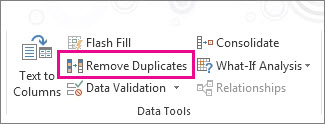
To remove duplicate values, click Data > Data Tools > Remove Duplicates.
To highlight unique or duplicate values, use the Conditional Formatting command in the Style group on the Home tab.

Filtering for unique values and removing duplicate values are two similar tasks, since the objective is to present a list of unique values. There is a critical difference, however: When you filter for unique values, the duplicate values are only hidden temporarily. However, removing duplicate values means that you are permanently deleting duplicate values.

A duplicate value is one in which all values in at least one row are identical to all of the values in another row. A comparison of duplicate values depends on the what appears in the cell—not the underlying value stored in the cell. For example, if you have the same date value in different cells, one formatted as «3/8/2006» and the other as «Mar 8, 2006», the values are unique.

Check before removing duplicates: Before removing duplicate values, it’s a good idea to first try to filter on—or conditionally format on—unique values to confirm that you achieve the results you expect.

Follow these steps:

Select the range of cells, or ensure that the active cell is in a table.
Click Data > Advanced (in the Sort & Filter group).
In the Advanced Filter popup box, do one of the following:

To filter the range of cells or table in place:

Click Filter the list, in-place.

To copy the results of the filter to another location:

Click Copy to another location.
In the Copy to box, enter a cell reference.
Alternatively, click Collapse Dialog to temporarily hide the popup window, select a cell on the worksheet, and then click Expand .
Check the Unique records only, then click OK.

The unique values from the range will copy to the new location.

When you remove duplicate values, the only effect is on the values in the range of cells or table. Other values outside the range of cells or table will not change or move. When duplicates are removed, the first occurrence of the value in the list is kept, but other identical values are deleted.

Because you are permanently deleting data, it’s a good idea to copy the original range of cells or table to another worksheet or workbook before removing duplicate values.

Follow these steps:

Select the range of cells, or ensure that the active cell is in a table.
On the Data tab, click Remove Duplicates (in the Data Tools group).
Do one or more of the following:
- Under Columns, select one or more columns.
- To quickly select all columns, click Select All.
- To quickly clear all columns, click Unselect All.
  
  If the range of cells or table contains many columns and you want to only select a few columns, you may find it easier to click Unselect All, and then under Columns, select those columns.
  
  Note: Data will be removed from all columns, even if you don’t select all the columns at this step. For example, if you select Column1 and Column2, but not Column3, then the “key” used to find duplicates is the value of BOTH Column1 & Column2. If a duplicate is found in those columns, then the entire row will be removed, including other columns in the table or range.
Click OK, and a message will appear to indicate how many duplicate values were removed, or how many unique values remain. Click OK to dismiss this message.
Undo the change by click Undo (or pressing Ctrl+Z on the keyboard).

Note: You cannot conditionally format fields in the Values area of a PivotTable report by unique or duplicate values.

Quick formatting

Follow these steps:

Select one or more cells in a range, table, or PivotTable report.
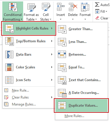
On the Home tab, in the Style group, click the small arrow for Conditional Formatting, and then click Highlight Cells Rules, and select Duplicate Values.
Enter the values that you want to use, and then choose a format.

Advanced formatting

Follow these steps:

Select one or more cells in a range, table, or PivotTable report.
On the Home tab, in the Styles group, click the arrow for Conditional Formatting, and then click Manage Rules to display the Conditional Formatting Rules Manager popup window.
Do one of the following:
- To add a conditional format, click New Rule to display the New Formatting Rule popup window.
- To change a conditional format, begin by ensuring that the appropriate worksheet or table has been chosen in the Show formatting rules for list. If necessary, choose another range of cells by clicking Collapse button in the Applies to popup window temporarily hide it. Choose a new range of cells on the worksheet, then expand the popup window again . Select the rule, and then click Edit rule to display the Edit Formatting Rule popup window.
Under Select a Rule Type, click Format only unique or duplicate values.
In the Format all list of Edit the Rule Description, choose either unique or duplicate.
Click Format to display the Format Cells popup window.
Select the number, font, border, or fill format that you want to apply when the cell value satisfies the condition, and then click OK. You can choose more than one format. The formats that you select are displayed in the Preview panel.

In Excel for the web, you can remove duplicate values.

Remove duplicate values

Important: You can always click Undo to get back your data after you have removed the duplicates. That being said, it’s a good idea to copy the original range of cells or table to another worksheet or workbook before removing duplicate values.

Follow these steps:

Select the range of cells, or ensure that the active cell is in a table.
On the Data tab, click Remove Duplicates .
In the Remove Duplicates dialog box, unselect any columns where you don’t want to remove duplicate values.

Note: Data will be removed from all columns, even if you don’t select all the columns at this step. For example, if you select Column1 and Column2, but not Column3, then the “key” used to find duplicates is the value of BOTH Column1 & Column2. If a duplicate is found in Column1 and Column2, then the entire row will be removed, including data from Column3.
Click OK, and a message will appear to indicate how many duplicate values were removed. Click OK to dismiss this message.

Note: If you want to get back your data, simply click Undo (or press Ctrl+Z on the keyboard).

Need more help?

You can always ask an expert in the Excel Tech Community or get support in the Answers community.

1 Answer

answered Jan 15, 2015 at 14:39

RFerwerdaRFerwerda

1,2672 gold badges10 silver badges24 bronze badges

Thanks but pnuts comment actually solved my problem. What I did wrong was that I didn’t select the whole sheet when I used the remove duplicate function. I had only selected the first column.

Jan 15, 2015 at 14:48

Источник

Watch Video – How to Find and Remove Duplicates in Excel

With a lot of data…comes a lot of duplicate data.

Duplicates in Excel can cause a lot of troubles. Whether you import data from a database, get it from a colleague, or collate it yourself, duplicates data can always creep in. And if the data you are working with is huge, then it becomes really difficult to find and remove these duplicates in Excel.

In this tutorial, I’ll show you how to find and remove duplicates in Excel.

FIND and HIGHLIGHT Duplicates in Excel.
- Find and Highlight Duplicates in a Single Column.
- Find and Highlight Duplicates in Multiple Columns.
- Find and Highlight Duplicate Rows.
REMOVE Duplicates in Excel.
- Remove Duplicates from a Single Column.
- Remove Duplicates from Multiple Columns.
- Remove Duplicate Rows.

Find and Highlight Duplicates in Excel

Duplicates in Excel can come in many forms. You can have it in a single column or multiple columns. There may also be a duplication of an entire row.

Finding and Highlight Duplicates in a Single Column in Excel

Conditional Formatting makes it simple to highlight duplicates in Excel.

Here is how to do it:

Select the data in which you want to highlight the duplicates.

Go to Home –> Conditional Formatting –> Highlight Cell Rules –> Duplicate Values.

In the Duplicate Values dialog box, select Duplicate in the drop down on the left, and specify the format in which you want to highlight the duplicate values. You can choose from the ready-made format options (in the drop down on the right), or specify your own format.

This will highlight all the values that have duplicates.

Quick Tip: Remember to check for leading or trailing spaces. For example, “John” and “John ” are considered different as the latter has an extra space character in it. A good idea would be to use the TRIM function to clean your data.

Finding and Highlight Duplicates in Multiple Columns in Excel

If you have data that spans multiple columns and you need to look for duplicates in it, the process is exactly the same as above.

Here is how to do it:

Select the data.
Go to Home –> Conditional Formatting –> Highlight Cell Rules –> Duplicate Values.
In the Duplicate Values dialog box, select Duplicate in the drop down on the left, and specify the format in which you want to highlight the duplicate values.
This will highlight all the cells that have duplicates value in the selected data set.

Finding and Highlighting Duplicate Rows in Excel

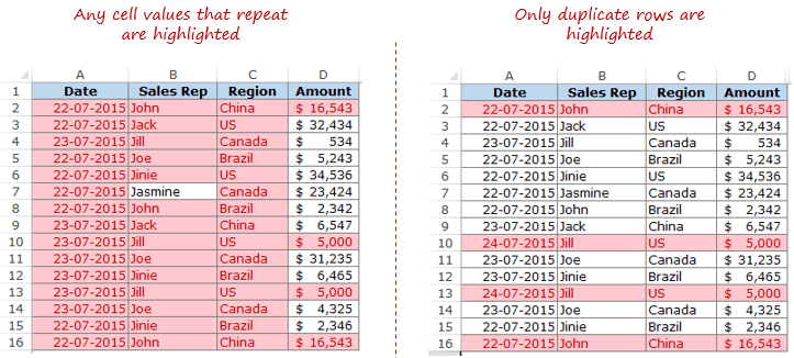
Finding duplicate data and finding duplicate rows of data are 2 different things. Have a look:

Finding duplicate rows is a bit more complex than finding duplicate cells.

Here are the steps:

In an adjacent column, use the following formula:
=A2&B2&C2&D2
Drag this down for all the rows. This formula combines all the cell values as a single string. (You can also use the CONCATENATE function to combine text strings)

By doing this, we have created a single string for each row. If there are duplicate rows in this dataset, then these strings would be exactly the same for it.

Now that we have the combined strings for each row, we can use conditional formatting to highlight duplicate strings. A highlighted string implies that the row has a duplicate.

Here are the steps to highlight duplicate strings:

Select the range that has the combined strings (E2:E16 in this example).
Go to Home –> Conditional Formatting –> Highlight Cell Rules –> Duplicate Values.
In the Duplicate Values dialog box, make sure Duplicate is selected and then specify the color in which you want to highlight the duplicate values.

This would highlight the duplicate values in column E.

In the above approach, we have highlighted only the strings that we created.

But what if you want to highlight all the duplicate rows (instead of highlighting cells in one single column)?

Here are the steps to highlight duplicate rows:

In an adjacent column, use the following formula:
=A2&B2&C2&D2
Drag this down for all the rows. This formula combines all the cell values as a single string.

Select the data A2:D16.
With the data selected, go to Home –> Conditional Formatting –> New Rule.

In the ‘New Formatting Rule’ dialog box, click on ‘Use a formula to determine which cells to format’.
In the field below, use the following COUNTIF function:
=COUNTIF($E$2:$E$16,$E2)>1

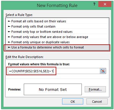
Select the format and click OK.

This formula would highlight all the rows that have a duplicate.

Remove Duplicates in Excel

In the above section, we learned how to find and highlight duplicates in excel. In this section, I will show you how to get rid of these duplicates.

Remove Duplicates from a Single Column in Excel

If you have the data in a single column and you want to remove all the duplicates, here are the steps:

Select the data.
Go to Data –> Data Tools –> Remove Duplicates.
In the Remove Duplicates dialog box:
- If your data has headers, make sure the ‘My data has headers’ option is checked.
- Make sure the column is selected (in this case there is only one column).

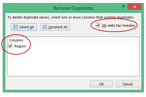
Click OK.

This would remove all the duplicate values from the column, and you would have only the unique values.

CAUTION: This alters your data set by removing duplicates. Make sure you have a back-up of the original data set. If you want to extract the unique values at some other location, copy this dataset to that location and then use the above-mentioned steps. Alternatively, you can also use Advanced Filter to extract unique values to some other location.

Remove Duplicates from Multiple Columns in Excel

Suppose you have the data as shown below:

In the above data, row #2 and #16 have the exact same data for Sales Rep, Region, and Amount, but different dates (same is the case with row #10 and #13). This could be an entry error where the same entry has been recorded twice with different dates.

To delete the duplicate row in this case:

Select the data.
Go to Data –> Data Tools –> Remove Duplicates.
In the Remove Duplicates dialog box:
- If your data has headers, make sure the ‘My data has headers’ option is checked.
- Select all the columns except the Date column.

Click OK.

This would remove the 2 duplicate entries.

NOTE: This keeps the first occurrence and removes all the remaining duplicate occurrences.

Remove Duplicate Rows in Excel

To delete duplicate rows, here are the steps:

Select the entire data.
Go to Data –> Data Tools –> Remove Duplicates.
In the Remove Duplicates dialog box:
- If your data has headers, make sure the ‘My data has headers’ option is checked.
- Select all the columns.

Click OK.

Use the above-mentioned techniques to clean your data and get rid of duplicates.

You May Also Like the Following Excel Tutorials:

10 Ways to Clean Data in Excel Spreadsheets.
Remove Leading and Trailing Spaces in Excel.
24 Daily Excel Issues and their Quick Fixes.
How to Find Merged Cells in Excel.

Источник

When you are working with spreadsheets in Microsoft Excel and accidentally copy rows, or if you are making a composite spreadsheet of several others, you will encounter duplicate rows which you need to delete. This can be a very mindless, repetitive, time-consuming task, but there are several tricks that make it simpler.

Getting Started

Today we will talk about a few handy methods for identifying and deleting duplicate rows in Excel. If you don’t have any files with duplicate rows now, feel free to download our handy resource with several duplicate rows created for this tutorial. Once you have downloaded and opened the resource, or opened your own document, you are ready to proceed.

Option 1 – Remove Duplicates in Excel

If you are using Microsoft Office, you will have a bit of an advantage because there is a built-in feature for finding and deleting duplicates.

Begin by selecting the cells you want to target for your search. In this case, we will select the entire table by pressing Ctrl+A on Windows or Command+A on Mac.

Once you have successfully selected the table, you will need to click on the Data tab on the top of the screen and then select “Remove Duplicates” in the Data Tools drop-down box as shown below.

Once you have clicked on it, a small dialog box will appear. You will notice that the first row has automatically been deselected. The reason for this is that the My Data Has Headers box is ticked.

In this case, we do not have any headers since the table starts at Row 1. We will deselect the My Data Has Headers box. Once you have done that, you will notice that the whole table has been highlighted again and the “Columns” section changed from “duplicates” to “Column A, B, and C.”

Now that the entire table is selected, you just press “OK” to delete all duplicates. In this case, all the rows with duplicate information except for one have been deleted and the details of the deletion are displayed in the popup dialog box.

RELATED: How to Remove Blank Rows in Excel

Option 2 – Advanced Filtering in Excel

The second tool you can use in Excel to Identify and delete duplicates is the Advanced Filter. This method also applies to Excel 2003. Let us start again by opening up the Excel spreadsheet. In order to sort your spreadsheet, you will need to first select all using Ctrl+A or Command+A as shown earlier.

After selecting your table, simply click the Data tab, and in the Sort & Filter section, click “Advanced.” If you are using Excel 2003, click Data > Filters, then choose “Advanced Filters.”

Now you will need to select the Unique Records Only check box.

Once you click “OK,” your document should have all duplicates except one removed. In this case, two were left because the first duplicates were found in Row 1.

This method automatically assumes that there are headers in your table. If you want the first row to be deleted, you will have to delete it manually in this case. If you actually had headers rather than duplicates in the first row, only one copy of the existing duplicates would have been left.

Option 3 – Replace

This method is great for smaller spreadsheets if you want to identify entire rows that are duplicated. In this case, we will be using the simple Replace tool that is built into all Microsoft Office products. You will need to begin by opening the spreadsheet you want to work on.

Once it is open, you need to select a cell with the content you want to find and replace and copy it. Click on the cell and press Ctrl+C on Windows or Command+C on Mac.

Once you have copied the word you want to search for, you will need to press Ctrl+H on Windows or Control+H on Mac to bring up the replace function. Once it is up, you can paste the word you copied into the Find What section by pressing Ctrl+V or Command+V.

Now that you have identified what you are looking for, press “Options.” Select the Match Entire Cell Contents checkbox. The reason for this is that sometimes your word may be present in other cells with other words. If you do not select this option, you could inadvertently end up deleting cells that you need to keep. Ensure that all the other settings match those shown in the image below.

Now you will need to enter a value in the Replace With box. For this example, we will use the number “1.” Once you have entered the value, press “Replace All.”

You will notice that all the values that matched “dulpicate” have been changed to “1.” The reason we used the number one is that it is small and stands out. Now you can easily identify which rows had duplicate content.

In order to retain one copy of the duplicates, simply paste the original text back into the first row that has been replaced by 1’s.

Now that you have identified all the rows with duplicate content, go through the document and hold Ctrl on Windows or Command on Mac while clicking on the number of each duplicate row as shown below.

Once you have selected all the rows that need to be deleted, right-click on one of the grayed-out numbers, and select “Delete.” The reason you need to do this instead of pressing the Delete key on your computer is that it will delete the rows rather than just the content.

Once you are done you will notice that all your remaining rows are unique values.

RELATED: How to Use Conditional Formatting to Find Duplicate Data in Excel

Удаление повторяющихся строк вручную

Если вы используете последнюю версию Microsoft Excel с 2007 по 2019, у вас есть небольшое преимущество. Эти версии содержат встроенную функцию для поиска и удаления повторяющихся значений.

Этот инструмент позволяет находить и удалять абсолютные совпадения (ячейки или целые строки), а также частично совпадающие записи (имеющие одинаковые значения в столбце или диапазоне).

Важно! Поскольку инструмент «Удалить дубликаты» навсегда удаляет идентичные записи, рекомендуется создать копию исходных данных, прежде чем удалять что-либо.

Для этого выполните следующие действия.

Для начала выберите диапазон, в котором вы хотите работать. Чтобы выделить всю таблицу, нажмите Ctrl + A,
Указав диапазон, перейдите на вкладку «Данные» > и нажмите кнопку «Удалить дубликаты» .

Откроется диалоговое окно. Выберите столбцы для проверки на наличие дублей и нажмите кнопку «ОК».
- Чтобы удалить повторяющиеся строки, которые имеют абсолютно одинаковые данные во всех колонках, оставьте флажки рядом со всеми столбцами, как на скриншоте ниже.
- Чтобы удалить частичные совпадения на основе одного или нескольких ключевых столбцов, выберите только их. Если в вашей таблице много колонок, самый быстрый способ — нажать кнопку «Снять выделение». А затем отметить те, которые вы хотите проверить.
- Ежели в вашей таблице нет заголовков, снимите флажок Мои данные в верхнем правом углу диалогового окна, который обычно включается по умолчанию.
Если указать в диалоговом окне все столбцы, строка будет удалена только в том случае, если повторяются значения есть во всех них. Но в некоторых ситуациях не нужно учитывать данные, находящиеся в определенных колонках. Поэтому для них снимите флажки. К примеру, если каждая строчка содержит уникальный идентификационный код, программа никогда не найдет ни одной повторяющейся. Поэтому флажок рядом с колонкой с такими кодами следует снять.

Выполнено! Все повторяющиеся строки в нашем диапазоне удаляются, и отображается сообщение, указывающее, сколько повторяющихся записей было удалено и сколько осталось уникальных.

Важное замечание. Повторяющиеся значения определяются по тому, что отображается в ячейке, а не по тому, что в ней записано на самом деле. Представим, что в A1 и A2 содержится одна и та же дата. Одна из них представлена в формате 15.05.2020, а другая отформатирована в формате 15 май 2020. При поиске повторяющихся значений Excel считает, что это не одно и то же. Аналогично значения, которые отформатированы по-разному, считаются разными, поэтому $1 209,32 — это совсем не одно и то же, что 1209,32.

Поэтому, для того чтобы обеспечить успешный поиск и удаление повторов в таблице или диапазоне данных, рекомендуется применить один формат ко всему столбцу.
Примечание. Функция удаления дублей убирает 2-е и все последующие совпадения, оставляя все уникальные и первые экземпляры идентичных записей.

Удаление дубликатов в «умной таблице».

Думаю, вы знаете, что, если преобразовать диапазон ячеек в таблицу, в нашем распоряжении появляется множество интересных дополнительных возможностей по работе с этими данными. Именно по этой причине такую таблицу Excel называют «умной».

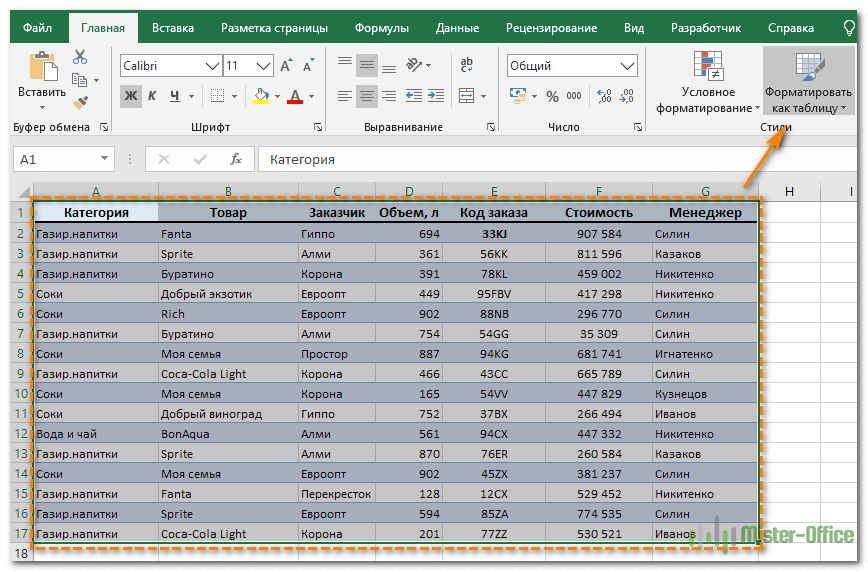
Выделите нужную нам область, затем на вкладке «Главная» выберите «Форматировать как таблицу». Далее вам будет предложено указать желаемый вариант оформления. Когда закончите, автоматически откроется вкладка «Конструктор».

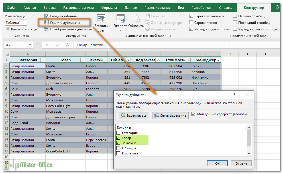
Выбираем на ленте нужную кнопку, как показано на скриншоте. Затем отмечаем те столбцы, в которых будем искать повторы. Ну а далее произойдет то же самое, что было описано в предыдущем разделе.

Но, в отличие от ранее рассмотренного инструмента удаления, операцию можно отменить, если что-то пошло не так.

Избавьтесь от повторов, скопировав уникальные записи в другое место.

Еще один способ удалить повторы — это выбрать все уникальные записи и скопировать их на другой лист или в другую книгу. Подробные шаги следуют ниже.

Выберите диапазон или всю таблицу, которую вы хотите обработать (1).
Перейдите на вкладку «Данные» (2) и нажмите кнопку «Фильтр — Дополнительно» (3-4).
В диалоговом окне «Расширенный фильтр» (5) выполните следующие действия:
- Выберите переключатель скопировать в другое место (6).
- Убедитесь, что в списке диапазонов указан правильный диапазон. Это должен быть диапазон из шага 1.
- В поле «Поместить результат в…» (7) введите диапазон, в который вы хотите скопировать уникальные записи (на самом деле достаточно указать его верхнюю левую ячейку).
- Выберите только уникальные записи (8).
Наконец, нажмите кнопку ОК, и уникальные значения будут скопированы в новое место:

Замечание. Расширенный фильтр позволяет копировать отфильтрованные данные в другое место только на активном листе. Например, выберите место внизу под вашими исходными данными.

Я думаю, вы понимаете, что можно обойтись и без копирования. Просто выберите опцию «Фильтровать список на месте», и дублирующиеся записи будут на время скрыты при помощи фильтра. Они не удаляются, но и мешать вам при этом не будут.

Как убрать дубликаты строк с помощью формул.

Еще один способ удалить неуникальные данные — идентифицировать их с помощью формулы, затем отфильтровать, а затем после этого удалить лишнее.

Преимущество этого подхода заключается в универсальности: он позволяет вам:

находить и удалять повторы в одном столбце,
находить дубликаты строк на основе значений в нескольких столбиках данных,
оставлять первые вхождения повторяющихся записей.

Недостатком является то, что вам нужно будет запомнить несколько формул.

В зависимости от вашей задачи используйте одну из следующих формул для обнаружения повторов.

Формулы для поиска повторяющихся значений в одном столбце

Добавляем еще одну колонку, в которой запишем формулу.

Повторы наименований товаров, без учета первого вхождения:

=ЕСЛИ(СЧЁТЕСЛИ($B$2:$B2; $B2)>1; «Дубликат»; «»)

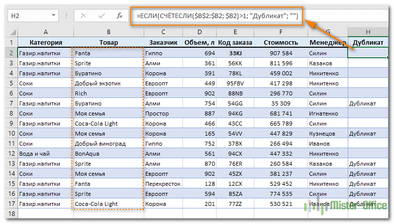
Как видите, когда значение встречается впервые (к примеру, в B4), оно рассматривается как вполне обычное. А вот второе его появление (в B7) уже считается повтором.

Отмечаем все повторы вместе с первым появлением:

=ЕСЛИ(СЧЁТЕСЛИ($B$2:$B$17; $B2)>1; «Дубликат»; «Уникальный»)

Где A2 — первая, а A10 — последняя ячейка диапазона, в котором нужно найти совпадения.

Ну а теперь, чтобы убрать ненужное, устанавливаем фильтр и в столбце H и оставляем только «Дубликат». После чего строки, оставшиеся на экране, просто удаляем.

Вот небольшая пошаговая инструкция.

Выберите любую ячейку и примените автоматический фильтр, нажав кнопку «Фильтр» на вкладке «Данные».
Отфильтруйте повторяющиеся строки, щелкнув стрелку в заголовке нужного столбца.
И, наконец, удалите повторы. Для этого выберите отфильтрованные строки, перетаскивая указатель мыши по их номерам, щелкните правой кнопкой мыши и выберите «Удалить строку» в контекстном меню. Причина, по которой вам нужно сделать это вместо простого нажатия кнопки «Удалить» на клавиатуре, заключается в том, что это действие будет удалять целые строки, а не только содержимое ячейки.

Формулы для поиска повторяющихся строк.

В случае, если нам нужно найти и удалить повторяющиеся строки (либо часть их), действуем таким же образом, как для отдельных ячеек. Только формулу немного меняем.

Отмечаем при помощи формулы неуникальные строчки, кроме 1- ^го вхождения:

=ЕСЛИ(СЧЁТЕСЛИМН($B$2:$B2; $B2;$A$2:A2;$A2;$C$2:C2;$C2)>1; «Дубликат»; «»)

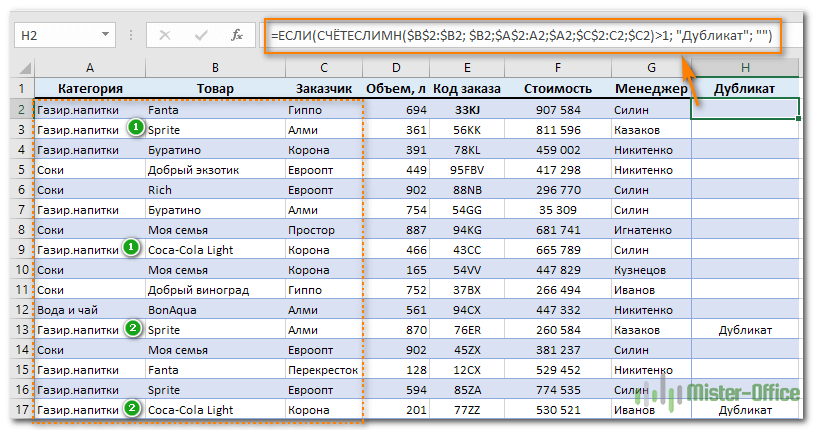
В результате видим 2 повтора.

Теперь самый простой вариант действий – устанавливаем фильтр по столбцу H и слову «Дубликат». После этого просто удаляем сразу все отфильтрованные строки.

Если нам нужно исключить все повторяющиеся строки вместе с их первым появлением:

=ЕСЛИ(СЧЁТЕСЛИМН($B$2:$B$17; $B2;$A$2:$A$17;$A2;$C$2:$C$17;$C2)>1; «Дубликат»; «»)

Далее вновь устанавливаем фильтр и действуем аналогично описанному выше.

Насколько удобен этот метод – судить вам.

Duplicate Remover — универсальный инструмент для поиска и удаления дубликатов в Excel.

В отличие от встроенной функции Excel для удаления дубликатов, о которой мы рассказывали выше, надстройка Ablebits Duplicate Remover не ограничивается только удалением повторяющихся записей. Подобно швейцарскому ножу, этот многофункциональный инструмент сочетает в себе все основные варианты использования и позволяет определять, выбирать, выделять, удалять, копировать и перемещать уникальные или повторяющиеся значения, с первыми вхождениями или без них, целиком повторяющиеся или частично совпадающие строки в одной таблице или путем сравнения двух таблиц.

Он безупречно работает во всех операционных системах и во всех версиях Microsoft Excel 2019 — 2003.

Как избавиться от дубликатов в Excel в 2 клика мышки.

Предполагая, что в вашем Excel установлен Ultimate Suite, выполните следующие простые шаги, чтобы удалить повторяющиеся строки или ячейки:

Выберите любую ячейку в таблице, c которой вы хотите работать, и нажмите Quick Dedupe на вкладке Ablebits Data.

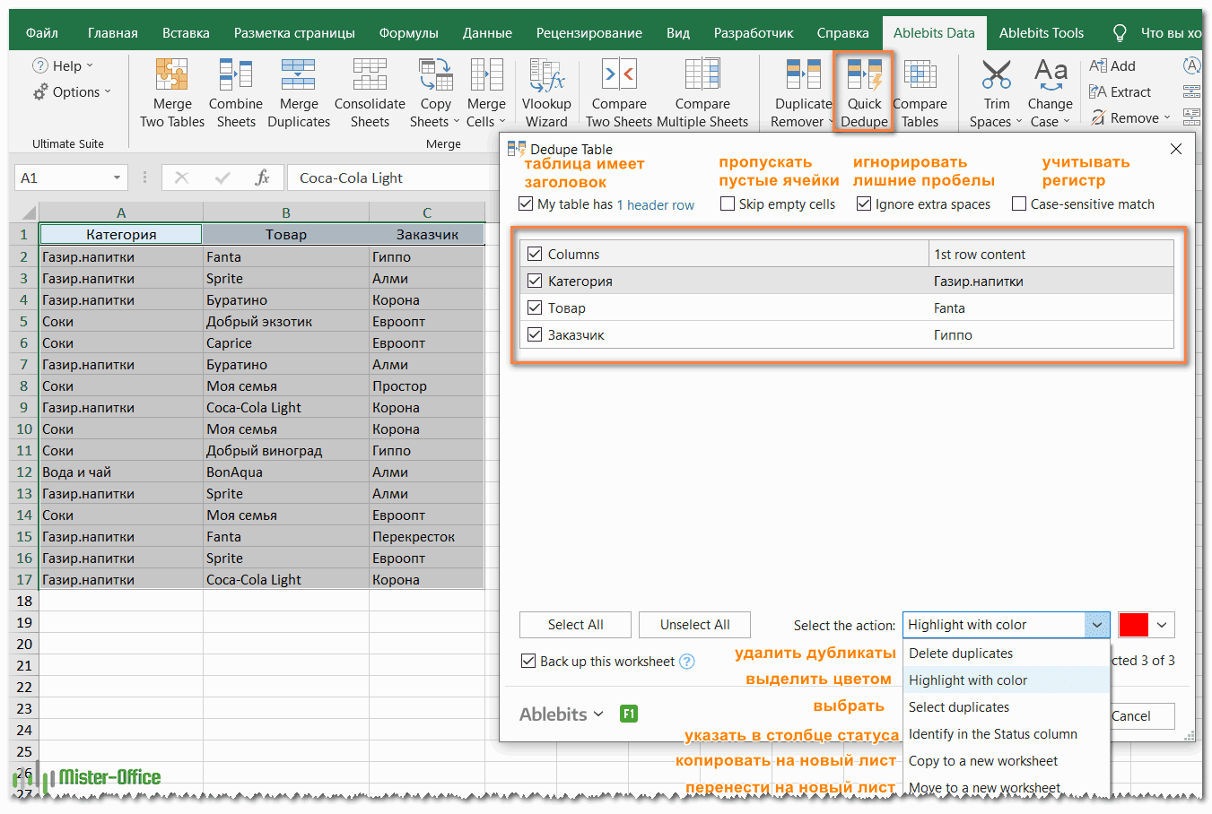
Откроется диалоговое окно, и все столбцы будут выбраны по умолчанию. Выберите те, которые вам нужны, а также в выпадающем списке в правом нижнем углу укажите желаемое действие.

Поскольку моя цель – просто выделить повторяющиеся данные, я выбрал «Закрасить цветом».

Помимо выделения цветом, вам доступны и другие операции:

Удалить дубликаты
Выбрать дубликаты
Указать их в столбце статуса
Копировать дубликаты на новый лист
Переместить на новый лист

Нажимаем кнопку OK и оцениваем получившийся результат:

Как вы можете видеть на скриншоте выше, строки с повторяющимися значениями в первых 3 столбцах были обнаружены (первые вхождения здесь по умолчанию не считаются как дубликаты).

Совет. Если вы хотите определить повторяющиеся строки на основе значений в ключевом столбце, оставьте выбранным только этот столбец (столбцы) и снимите флажки со всех остальных неактуальных столбцов.

И если вы хотите выполнить какое-то другое действие, например, удалить повторяющиеся строки, или скопировать повторяющиеся значения в другое место, выберите соответствующий вариант из раскрывающегося списка.

Больше возможностей для поиска дубликатов при помощи Duplicate Remover.

Если вам нужны дополнительные параметры, такие как удаление повторяющихся строк, включая первые вхождения, или поиск уникальных значений, используйте мастер Duplicate Remover, который предоставляет эти и некоторые другие возможности. Рассмотрим на примере, как найти повторяющиеся значения с первым вхождением или без него.

Удаление дубликатов в Excel — обычная операция. Однако в каждом конкретном случае может быть ряд особенностей. В то время как инструмент Quick Dedupe фокусируется на скорости, Duplicate Remover предлагает ряд дополнительных опций для работы с дубликатами и уникальными значениями.

Выберите любую ячейку в таблице, где вы хотите удалить дубликаты, переключитесь на вкладку Ablebits Data и нажмите кнопку Duplicate Remover.

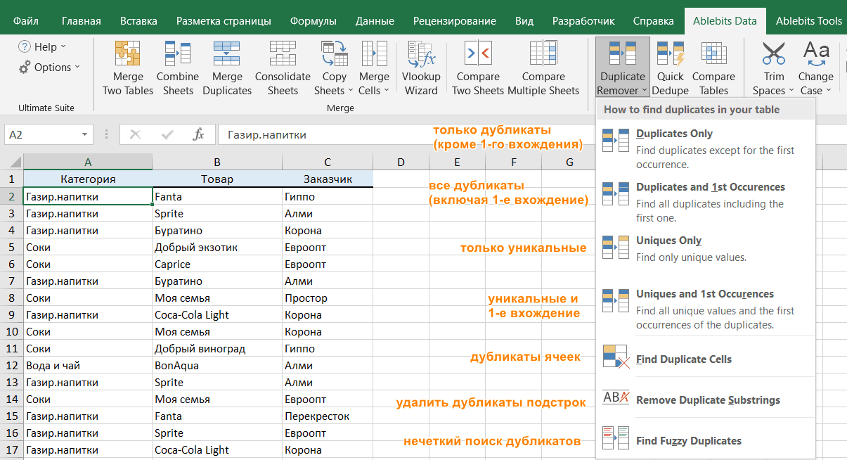
Вам предложены 4 варианта проверки дубликатов в вашем листе Excel:
- Дубликаты без первых вхождений повторяющихся записей.
- Дубликаты с 1-м вхождением.
- Уникальные записи.
- Уникальные значения и 1-е повторяющиеся вхождения.
В этом примере выберем второй вариант, т.е. Дубликаты + 1-е вхождения:

Все ваши данные будут автоматически выделены.
Теперь выберите столбцы, в которых вы хотите проверить дубликаты. Как и в предыдущем примере, мы выбираем первые 3 столбца:

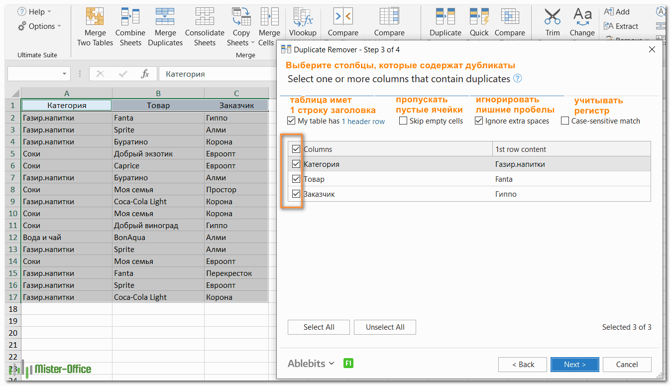
Наконец, выберите действие, которое вы хотите выполнить с дубликатами. Как и в случае с инструментом быстрого поиска дубликатов, мастер Duplicate Remover может идентифицировать, выбирать, выделять, удалять, копировать или перемещать повторяющиеся данные.

Чтобы более наглядно увидеть результат, отметим параметр «Закрасить цветом» (Fill with color) и нажимаем Готово.

Мастеру Duplicate Remover требуется совсем немного времени, чтобы проанализировать вашу таблицу и показать результат:

Как видите, результат аналогичен тому, что мы наблюдали выше. Но здесь мы выделили дубликаты, включая и первое появление этих повторяющихся записей. Если вы выберете опцию удаления, то эти 4 записи будут стерты из вашей таблицы.

Надстройка также создает резервную копию рабочего листа, чтобы случайно не потерять нужные данные: вдруг вы хотели оставить первые вхождения данных, но случайно выбрали не тот пункт.

Мы рассмотрели различные способы, которыми вы можете убрать дубликаты из ваших таблиц — при помощи формул и без них. Я надеюсь, что хотя бы одно из решений, упомянутых в этом обзоре, вам подойдет.

Все мощные инструменты очистки дублей, описанные выше, включены в надстройку Ultimate Suite для Excel. Если вы хотите попробовать их, я рекомендую вам загрузить полнофункциональную пробную версию и сообщить нам свой отзыв в комментариях.

Что ж, как вы только что видели, есть несколько способов найти повторяющиеся значения в Excel и затем удалить их. И каждый из них имеет свои сильные стороны и ограничения.

Еще на эту же тему:

Источник

Filter for unique values or remove duplicate values

Remove duplicate values

Need more help?

See Also

Need more help?

1 Answer

CONTENTS:

Find and Highlight Duplicates in Excel

Finding and Highlight Duplicates in a Single Column in Excel

Finding and Highlight Duplicates in Multiple Columns in Excel

Finding and Highlighting Duplicate Rows in Excel

Remove Duplicates in Excel

Remove Duplicates from a Single Column in Excel

Remove Duplicates from Multiple Columns in Excel

Remove Duplicate Rows in Excel

Getting Started

Option 1 – Remove Duplicates in Excel

Option 2 – Advanced Filtering in Excel

Option 3 – Replace

Удаление повторяющихся строк вручную

Удаление дубликатов в «умной таблице».

Избавьтесь от повторов, скопировав уникальные записи в другое место.

Как убрать дубликаты строк с помощью формул.

Формулы для поиска повторяющихся значений в одном столбце

Формулы для поиска повторяющихся строк.

Duplicate Remover — универсальный инструмент для поиска и удаления дубликатов в Excel.

Как избавиться от дубликатов в Excel в 2 клика мышки.

Больше возможностей для поиска дубликатов при помощи Duplicate Remover.