
Conditional Formatting in Excel enables you to quickly format a cell (or range of cells) based on the value or the text in it.
For example, below I have an example where I have student’s scores and I have used conditional formatting to highlight all the scores that are above 80.
If you’re interested in learning all the amazing things you can do with conditional formatting, check out this tutorial where I show some useful conditional formatting examples.
Once you have set the conditional formatting rules for a cell or range of cells, you can easily copy it to other cells on the same sheet or other sheets.
In this tutorial, I will show you how to copy conditional formatting from one cell to another cell in Excel. I will cover multiple ways to do this – such as simple copy-paste, copy and paste conditional formatting only, and using the format painter.
So let’s get started!
Copy Conditional Formatting Using Paste Special
Just like you can copy and paste cells in the same sheet or even across sheets or workbooks, you can also copy and paste the conditional formatting from one cell to another.
Note that you can not just copy and paste the cell. You have to make sure that you copy a cell but only paste the conditional formatting rules in that cell (and not everything else such as the value or the formula).
And to make sure you only copy and paste the conditional formatting, you need to use Paste Special.
Suppose you have a dataset as shown below where I have conditional formatting applied to column B (the Math score) so that all the cells that have the value more than 80 get highlighted.

Now, what if I want to apply the same conditional formatting rule to the second column (for Physics score) os that all the cells above 80 are highlighted in green.
This can easily be done!
Below are the steps to copy conditional formatting from one cell to another:
- Select cell B2
- Right-click and copy it (or use the keyboard shortcut Control + C)

- Select the entire range where you want to copy the conditional formatting (C2:C11 in this example)
- Right-click anywhere in the selection
- Click on the Paste Special option. This will open the Paste Special dialog box.

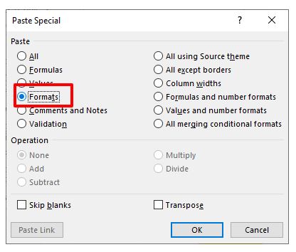
- In the Paste Special dialog box, select Formats

- Click on OK


The above steps would copy the conditional formatting from column B and apply it to the selected cells in column C.

One thing to remember when using Paste Special to copy conditional formatting is that it will copy all the formatting. So if there is any border in the cells or if the text has been made bold, etc., that would also be copied.
Note: The same steps shown above would also work when copying and pasting conditional formatting to cells in another sheet or even another workbook.
Copy Conditional Formatting Using Format Painter
Format painter is a tool that allows you to copy the format from a cell (or range of cells) and paste it.
And since conditional formatting is also a part of the formatting, you can also use format painter to copy and then paste it.
Suppose you have a dataset as shown below where I have conditional formatting applied to the Math score column so that all the cells that have the value more than 80 get highlighted.
Below are the steps to use format painter to copy conditional formatting from the Math score column and apply it to the Physics score column:
- Select the cell (or range of cells) from which you want to copy the conditional formatting
- Click the Home tab
- In the Clipboard group, click on the Format Painter icon

- Select all the cells where you want the copied conditional formatting to be applied


Pro tip: In case you want to copy the conditional formatting and paste it on multiple cells or ranges (that you can not select at one go), click on the Format painter icon twice. That will keep the format painter active and you can paste the formatting multiple times (unless you hit the Escape key).
Once you have the format painter activated, you can use it on the same sheet, on some other sheet in the same workbook, and even on the other workbook.
Again, just like with paste special, Format painter also copies all the formatting (including the conditional formatting).
Issue when Copying Conditional Formatting
In most cases, you will have no problems copying and pasting conditional formatting from one cell to another.
But you may face issues if you have used a custom formula to determine which cells to format.
This option allows you to create your own formula and formatting is applied in the formula returns TRUE for a cell and not applied when the formula returns FALSE.
If you have used a formula in conditional formatting that uses absolute or mixed references, then it may not work as expected when copied.
For example, in the below example, I have used the formula =$B2>=80 to highlight all cells in column B that have a value higher than 80.

But when I copy this conditional formatting to column C, it still references the B column and I get the wrong result (as shown below).

So, if you copy conditional formatting from one cell to another and don’t get the expected result, it’s best to check the formula used and adjust the references.
For example, in this case, I can change the formula to =B2>=80 and it should work fine.
If you’re wondering where the formula goes, click on the Home tab and then on Conditional Formatting.
In the options that appear, click on ‘New Rule’. In the New Formatting Rule dialog box, click on the option – Use a formula to determine which cells to format.
This will show you the field where you can enter the formula for the selected range. If this formula returns TRUE for the cell, it will get formatted and if it returns FALSE, it will not.

So these are two simple ways you can use to copy conditional formatting from one cell to another in Excel – using Paste Special and Format Painter.
And in case you see issues with it, check the custom formula used in it.
Hope you found this tutorial useful!
Other Excel tutorials you may find useful:
- Highlight Rows Based on a Cell Value in Excel (Conditional Formatting)
- Highlight EVERY Other ROW in Excel (using Conditional Formatting)
- How to Remove Table Formatting in Excel
- Search and Highlight Data Using Conditional Formatting
- How to Apply Conditional Formatting in a Pivot Table in Excel
- Highlight the Active Row and Column in a Data Range in Excel
- Apply Conditional Formatting Based on Another Column in Excel
- Copy and Paste Multiple Cells in Excel (Adjacent & Non-Adjacent)
Conditional formatting is a feature of Excel which allows you to apply a format such as colors, icons, and data bars to a cell or a range of cells based on certain criteria. There are many ways to use Conditional Formatting, and you can also copy that format to another cell.
Basic Conditional Formatting
If you want to highlight the cell based on a value of a specified cell as criteria, then you can use conditional formatting with a custom formula.
In the example below, you will set conditional formats so that a cell:
- Turns green if it contains a value higher than 100 and
- Turns red if it contains a value equal to 50.
- Turns blue if it contains a value less than 20.
Conditional format if a cell contains a value higher than 100
Select the range you want to format. In our case A2:A15 is selected. On the Ribbon’s Home tab, click Conditional Formatting, to format the values greater than a specific one select Highlight Cells Rules and then choose the option Greater Than.
To drop down the list for formats click Custom Format, click the Fill tab, and click on the green fill color that you want. To close the Format Cells window click Ok, the cells with values greater than 100 now are colored green as we choose the color format.

In the A column could be 100 as a value and using the format we used above the 100 value so it won’t be highlighted, including 100 in highlighted values we should use another format rule.
Conditional formatting if it contains a value less than 20.

To color the low values in blue fill, you can apply a second conditional formatting rule to the cells. Select the cells to be formatted. In this example, cells A2:A15 are selected then on the Ribbon’s Home tab, click Conditional Formatting.

To format the less than values, click highlight cell rules, then click less than. In the less than the window, delete the value that appears, and click on cell C2, where the low value is entered.

Click the drop-down list for formats, and click Custom Format. In the Format Cells window, click the Fill tab, and click on the green fill color that you want.
Click OK to close the Format Cells window, and click OK to close the Less Than window. The cells with values greater than 100 are now colored green, and cells less than 20 are blue.

Conditional formatting if it contains a value is equal with 50.
Select the cells to be formatted. In this example, cells A2:A15 are selected, From the Home tab, click the Conditional Formatting command. A drop-down menu will appear to click Highlight Cell Rules and then choose Equal to.
In the Equal to the window, you have to delete the value that appears in the box, and then select the cell in this example C3 cell or a specific value in our case 50.
After choosing our desired format press OK and A6 cell which equals 50 will be formatted.


Conditional format if cell contains text
To auto-fill a cell with color in Excel given that it has text in it you can achieve this by applying conditional formatting and selecting a Rule Type for your range of values.
Do the following steps:
Select the range of cells for your data, like A1:A15. Then in the Home tab, go to Conditional Formatting, click on “New Rules” select the rule type as “Use a Formula to determine which cells to format” write the following formula, in formula section. Remember to give reference of the only 1st cell of your selected range of cells.
=ISTEXT(A1)

Click on “Format” button, In “Fill” tab, select the color for the text values you want to format with, click OK, and again click OK on new formatting rule window
You will get all the text values in your selected range of cells to be filled with your desired color scheme.

To highlight entire rows of cells containing the specific text, value or just be blank with the Conditional Formatting command in Excel, you can do as following:
Select the purchase table without its column headings. Click the Home > Conditional Formatting > New Rule


In the coming New Formatting Rule dialog box click to select the “Use a formula to determine” which cells to format in the select a rule type box:
In the format values where this formula is the true box, enter =$A1=”Apple” click the Format button.
In the formula of =$A1=”Apple,” $A1 is the cell you will check if contains the specific text or value, and “Apple” is the specific text, you can change them as you need. And this formula can only find out cells only containing the specific text or value.

If you want to highlight rows if cells begin with the specific text, you need to enter =LEFT($A1,5)=”Apple”; or to highlight rows if cells end with specific text, enter =RIGHT($A1,5)=”Apple.”

Now the Format Cells dialog box is opening. Go to the Fill tab, specify a background color, and click the OK button.
Click OK button to close the New Formatting Rule dialog box.
Then all rows containing the specific content cells in the selected range are highlighted if a $ sign is written before A(column) in the formula.
Copying Conditional Formatting to Another Cell
If you apply a conditional format to one or more cells and want to apply that format to other data on your worksheet, use Format Painter to copy the conditional formatting to that data.
Click on the cell that has the conditional formatting you want to copy. Click Home > Format Painter.

To paste the conditional formatting, drag the paintbrush across the cells or ranges of cells you want to format.
There are multiple ways you can specify the conditional format in a cell. You can even apply conditional format on one cell based on other cells criteria. The conditional format can also be applied to the whole row or column. For a customized solution to your specific problem, you can try our Excel expert help service using this link. It will save you hours of searching online and our expert will solve your problem in a 20-minute session. The first question is free.
Are you still looking for help with Conditional Formatting? View our comprehensive round-up of Conditional Formatting tutorials here.
The number of convenience stores everywhere is a true indicator of how much we revel in convenience. Excel agrees with the lot of us and harbors many such conveniences with multiple methods.
Sticking to that theme, today’s tutorial welcomes you to learn about copying Conditional Formatting in Excel. The highlights of this how-to are using Paste Special, the Format Painter, and the Conditional Formatting Rules Manager to copy Conditional Formatting, also touching on a small issue you may face with this Excel feature.
So without further ado, lets dive in.
 1")
Why would you want to copy Conditional Formatting?
You have sales data split branch-wise and have highlighted the figures less than $100 a day. You want to copy the same Conditional Formatting of this data for a newly added branch. Or you could have highlighted alternate rows and want the same highlighting for an added column.
Basically when you copy Conditional Formatting, you’re copying a Conditional Formatting Rule. The condition or criterion specified in that rule allows the new range to take on the format according to its own values. What will be copied from the copy area is not the static format, but the criteria of the Conditional Formatting Rule which will then format the paste area accordingly.
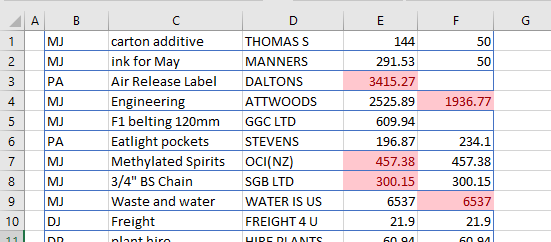
Simple copy-pasting will result in ditto pasting of the value, Conditional Formatting Rule, and the format of the cell(s). See this data below with Conditional Formatting applied to one column:
 2")
If we copy the numbers from column C to columns D, E, and F, the latter columns will be overwritten:
 3")
Therefore, you will have to employ one of the methods in this tutorial to copy the format. It’s not only highlighting that you can copy; any Conditional Formatting item can be copied. Highlighting, Data Bars, Color Scales, and Icon Sets; all these items will be copied the same way. Highlighted data like this:
 4")
And Data Bars like this:
 5")
Their formats will be copied no differently! Allow us to demonstrate.
Let’s get copying!
Using Paste Special
The prime instinct of copying anything is to copy-paste it but not everything is a Ctrl + C, Ctrl + V situation. Those situations, including Conditional Formatting, require pasting a little specially. The Paste Special options in Excel include pasting the format from copied cells.
The steps ahead use an example to copy Data Bars from one column to another. The sales figures for the year 2025 have been visually enhanced with Conditional Formatting’s Data Bars. The aim is to copy the format from the sales for 2025 to 2026. Use the following steps to copy the Conditional Formatting with Paste Special.
- Select the cells that you want to copy the format from.
 6")
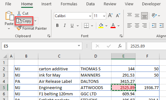
- Copy the selected cells by pressing the Ctrl + C
 7")
- Select the range where the Conditional Formatting is to be pasted.
- Right-click the selection and point to Paste Special from Paste Options in the opened context menu.
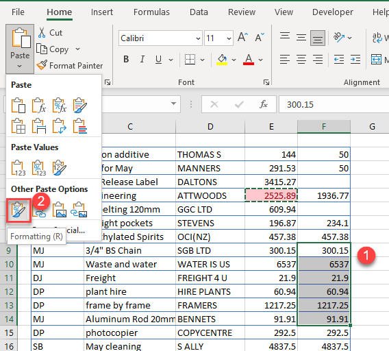
- Under Other Paste Options, click on the Formatting button.
 8")
Alternatively use the keyboard shortcut Alt + e + s + t + Enter after selecting the paste area. The Alt + e + s keys open the Paste Special dialog box, t will select the Formats radio button and the Enter key will select the OK command.
Whether you opt for the right-click context menu or the keyboard shortcut, the copied cells will render their format to the selected range for pasting:
 9")
Note in the sample shot above that the Data Bars have been pasted according to the cell values in the paste range. This also holds true for the other types of Conditional Formatting; if a value in one list is highlighted, the copied format won’t highlight the paste range according to the copied range’s values but according to the paste range’s values.
Using Format Painter
The Format Painter has one job; painting the format from one point to another. Sounds like we can work with that. The Format Painter can pick up on Conditional Formatting and paint/paste the format to a range of choice. Find out how to copy Conditional Formatting using the Format Painter with these steps:
- Select the range with the preferred format.
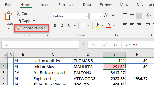
- Click on the Format Painter button (double-click for using the Format Painter for multiple points) in the Home tab’s Clipboard
 10")
- The cursor will be changed to a cross with a paintbrush icon.
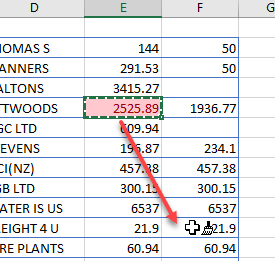
- To apply the format, select the area that you want to paint the copied format to with the new cursor.
 11")
The Format Painter will paint the format to the new selection:
Using the Conditional Formatting Rules Manager
The third option for copying a Conditional Formatting Rule is to duplicate the rule in Conditional Formatting’s Rules Manager. The Duplicate Rule option in the Rules Manager will exactly copy a rule and you can then edit the range it is applied to. Let’s show you how to copy Conditional Formatting using the Rules Manager with our case example:
- To open the Rules Manager, use the Conditional Formatting button in the Home tab’s Style group and select Manage Rules from the menu.
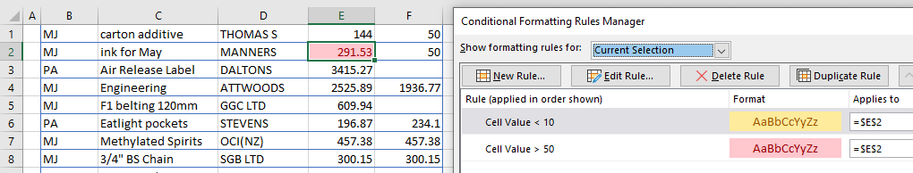
- The Show formatting rules for bar shows Current Selection. Change it to This Worksheet to view the rules for the current worksheet.
 13")
- Select the rule that you want to copy and click on the Duplicate Rule button from the bar at the top.
- This will create an identical Conditional Formatting Rule.
 14")
- Click on the Applies to field to edit the reference.
- In our example case, we will change the reference from C3:C14 to D3:D14. You can do this manually or you can select the new range on the worksheet after clicking on the Applies to field.
- When done, click on the OK button of the Rules Manager.
The duplicated rule with the altered cell reference copies the Conditional Formatting to the sales figures in column D:
 15")
Issues when Copying Conditional Formatting
Conditional Formatting is a pretty smart feature that shouldn’t usually cause any bother. The possibility of bother comes with using custom formulas in the Rules. The problem that you may see with custom formulas is static formatting.
That means when you will try to copy the formatting from, let’s say, column A to column B, it will be the same in both columns implying that Conditional Formatting is only accounting for the values in column A and not column B. This is not Conditional Formatting malfunctioning and there’s a small reason behind the appearance of this issue.
Let’s see what this issue looks like with a new example.
In our example, we have the monthly sales for the quarter also categorized by the sales representatives. Employees who managed sales at or above $1,600 will receive a bonus. For the first month, we already applied a Conditional Formatting Rule to highlight the sales at or exceeding $1,600 and things are alright at this point.
But when we tried copying the conditional format, here’s what happened:
 17")
In one glance, we know that’s not right. You can see that the sales figures in February, March, and April are highlighted in a linear pattern extending from column A. The sales greater than and equal to $1,600 have not been highlighted and the focus of the copied format is only visual.
As to why that’s happening, let’s check the particulars of the Conditional Formatting Rule. Select a cell from column A’s sales and go to Home tab > Conditional Formatting icon > Manage Rules. In the launched Rules Manager, select the relevant rule and hit the Edit Rule button.
There’s the culprit:
 18")
The formula entered for this rule is as follows:
=$C6>=1600
Column C is locked as an absolute reference while the row is free. This type of cell reference is fed into the formula when you want to highlight the full row of the cell that meets the condition of the formula.
If we convert the absolute reference into a relative one, the new formula would be as follows:
=C6>=1600
This keeps the row and column, both relative. Close the dialog box and the Rules Manager by selecting the OK buttons.
Now the correct figures have been highlighted from the edited Conditional Formatting Rule:
 19")
A few ways of copying Conditional Formatting, a small troubleshooter on an issue with copying Conditional Formatting, bagged it! More items for your Excel baggage? Coming up!
See all How-To Articles
This tutorial demonstrates how to copy conditional formatting rules in Excel and Google Sheets.
► Click here to jump to the Google Sheets walkthrough.
Copy Conditional Formatting
If you set up conditional formatting rules correctly, you can use the format painter or Paste Special to copy the rule to other cells in a worksheet.
Format Painter
- Select the cell that has a conditional formatting rule and then, in the Ribbon, go to Home > Clipboard > Format Painter.
- Click on the destination cell to apply the conditional formatting rule.
Paste Special
- Click on the cell with the conditional formatting rule applied, and then in the Ribbon, go to Home > Clipboard > Copy.
- Highlight the cell or cells to copy the conditional formatting rule to, and then in the Ribbon, go to Home > Paste > Other Paste Options > Formatting.
Alternatively, go to Paste > Other Paste Options > Paste Special. Choose Formats and click OK.
Copy Conditional Formatting in Google Sheets
Copying conditional formatting rules in Google Sheets is just like doing it in Excel.
Paint Format
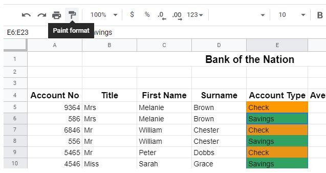
- Click on the cell that contains the conditional formatting rules.
- Click Paint format, and then highlight the cells to copy the conditional formatting rules to.
Paste Special
- Click on the cell that contains the conditional formatting rules, and in the Menu, go to Edit > Copy.
- Highlight the cells where you want the formatting to be copied to, and then in the Menu, go to Edit > Paste Special > Paste conditional formatting only.
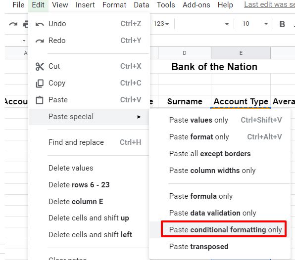
The conditional formatting rules are applied to the selected cells.

Содержание
- How to Copy Conditional Formatting in Excel & Google Sheets
- Copy Conditional Formatting
- Format Painter
- Paste Special
- Copy Conditional Formatting in Google Sheets
- Paint Format
- Paste Special
- Copy and remove
- Want more?
- How to Copy Conditional Formatting to Another Cell in Excel
- Copy Conditional Formatting Using Paste Special
- Copy Conditional Formatting Using Format Painter
- Issue when Copying Conditional Formatting
- How to copy conditional formating to another Excel Worksheet
- 4 Answers 4
- How to Copy Conditional Formatting in Microsoft Excel
- Copy Formatting Using Format Painter
- Copy Formatting Using Paste Special
- Copy Formatting Using the Conditional Formatting Rules Manager
How to Copy Conditional Formatting in Excel & Google Sheets
This tutorial demonstrates how to copy conditional formatting rules in Excel and Google Sheets.
► Click here to jump to the Google Sheets walkthrough.
Copy Conditional Formatting
If you set up conditional formatting rules correctly, you can use the format painter or Paste Special to copy the rule to other cells in a worksheet.
Format Painter
- Select the cell that has a conditional formatting rule and then, in the Ribbon, go to Home >Clipboard > Format Painter.
- Click on the destination cell to apply the conditional formatting rule.
Paste Special
- Click on the cell with the conditional formatting rule applied, and then in the Ribbon, go to Home > Clipboard > Copy.
- Highlight the cell or cells to copy the conditional formatting rule to, and then in the Ribbon, go to Home > Paste > Other Paste Options > Formatting.
Alternatively, go to Paste > Other Paste Options > Paste Special. Choose Formats and click OK.
Copy Conditional Formatting in Google Sheets
Copying conditional formatting rules in Google Sheets is just like doing it in Excel.
Paint Format
- Click on the cell that contains the conditional formatting rules.
- Click Paint format, and then highlight the cells to copy the conditional formatting rules to.
Paste Special
- Click on the cell that contains the conditional formatting rules, and in the Menu, go to Edit > Copy.
- Highlight the cells where you want the formatting to be copied to, and then in the Menu, go to Edit > Paste Special > Paste conditional formatting only.
The conditional formatting rules are applied to the selected cells.
Источник
Copy and remove

This video shows you how to quickly copy a cell’s formatting, remove conditional formatting from specific cells, and remove all conditional formatting from an entire worksheet.
Copy conditional formatting
If you have a conditional formatting rule that you want to use for new data, copy the conditional formatting to the new data using the Format Painter.
Click a cell that has the conditional formatting you want to copy.
Click HOME > Format Painter. The pointer changes to a paintbrush. Double-click Format Painter if you want to copy the formatting to multiple selections.
To copy the formatting, drag the mouse pointer across the cells or ranges of cells that you want to format.
To stop the formatting, press Esc.
Want more?
I’ve already applied conditional formatting to cell B2. If the cell contains the text “oil”, the cell’s formatting is red.
To copy the cell’s formatting, I select the cell, click Format Painter on the HOME tab, and select the cells I want to format.
To remove conditional formatting from specific cells, select the cells, click the Quick Analysis button, and click Clear Format.
To remove all conditional formatting from the entire worksheet,click the Conditional Formatting button on the HOME tab, point to Clear Rules, and click Clear Rules from Entire Sheet.
Now, you have got a pretty good idea about how to apply conditional formatting.
Of course, there is always more to learn.
So check out the course summary at the end, and best of all, explore Excel 2013 on your own.
Источник
How to Copy Conditional Formatting to Another Cell in Excel
Conditional Formatting in Excel enables you to quickly format a cell (or range of cells) based on the value or the text in it.
For example, below I have an example where I have student’s scores and I have used conditional formatting to highlight all the scores that are above 80.
If you’re interested in learning all the amazing things you can do with conditional formatting, check out this tutorial where I show some useful conditional formatting examples.
Once you have set the conditional formatting rules for a cell or range of cells, you can easily copy it to other cells on the same sheet or other sheets.
In this tutorial, I will show you how to copy conditional formatting from one cell to another cell in Excel. I will cover multiple ways to do this – such as simple copy-paste, copy and paste conditional formatting only, and using the format painter.
So let’s get started!
This Tutorial Covers:
Copy Conditional Formatting Using Paste Special
Just like you can copy and paste cells in the same sheet or even across sheets or workbooks, you can also copy and paste the conditional formatting from one cell to another.
Note that you can not just copy and paste the cell. You have to make sure that you copy a cell but only paste the conditional formatting rules in that cell (and not everything else such as the value or the formula).
And to make sure you only copy and paste the conditional formatting, you need to use Paste Special.
Suppose you have a dataset as shown below where I have conditional formatting applied to column B (the Math score) so that all the cells that have the value more than 80 get highlighted.
Now, what if I want to apply the same conditional formatting rule to the second column (for Physics score) os that all the cells above 80 are highlighted in green.
This can easily be done!
Below are the steps to copy conditional formatting from one cell to another:
- Select cell B2
- Right-click and copy it (or use the keyboard shortcut Control + C)

- Select the entire range where you want to copy the conditional formatting (C2:C11 in this example)
- Right-click anywhere in the selection
- Click on the Paste Special option. This will open the Paste Special dialog box.
- In the Paste Special dialog box, select Formats
- Click on OK
The above steps would copy the conditional formatting from column B and apply it to the selected cells in column C.
One thing to remember when using Paste Special to copy conditional formatting is that it will copy all the formatting. So if there is any border in the cells or if the text has been made bold, etc., that would also be copied.
Note: The same steps shown above would also work when copying and pasting conditional formatting to cells in another sheet or even another workbook.
Copy Conditional Formatting Using Format Painter
Format painter is a tool that allows you to copy the format from a cell (or range of cells) and paste it.
And since conditional formatting is also a part of the formatting, you can also use format painter to copy and then paste it.
Suppose you have a dataset as shown below where I have conditional formatting applied to the Math score column so that all the cells that have the value more than 80 get highlighted.
Below are the steps to use format painter to copy conditional formatting from the Math score column and apply it to the Physics score column:
- Select the cell (or range of cells) from which you want to copy the conditional formatting
- Click the Home tab
- In the Clipboard group, click on the Format Painter icon
- Select all the cells where you want the copied conditional formatting to be applied
Pro tip: In case you want to copy the conditional formatting and paste it on multiple cells or ranges (that you can not select at one go), click on the Format painter icon twice. That will keep the format painter active and you can paste the formatting multiple times (unless you hit the Escape key).
Once you have the format painter activated, you can use it on the same sheet, on some other sheet in the same workbook, and even on the other workbook.
Again, just like with paste special, Format painter also copies all the formatting (including the conditional formatting).
Issue when Copying Conditional Formatting
In most cases, you will have no problems copying and pasting conditional formatting from one cell to another.
But you may face issues if you have used a custom formula to determine which cells to format.
This option allows you to create your own formula and formatting is applied in the formula returns TRUE for a cell and not applied when the formula returns FALSE.
If you have used a formula in conditional formatting that uses absolute or mixed references, then it may not work as expected when copied.
For example, in the below example, I have used the formula =$B2>=80 to highlight all cells in column B that have a value higher than 80.
But when I copy this conditional formatting to column C, it still references the B column and I get the wrong result (as shown below).
So, if you copy conditional formatting from one cell to another and don’t get the expected result, it’s best to check the formula used and adjust the references.
For example, in this case, I can change the formula to =B2>=80 and it should work fine.
If you’re wondering where the formula goes, click on the Home tab and then on Conditional Formatting.
In the options that appear, click on ‘New Rule’. In the New Formatting Rule dialog box, click on the option – Use a formula to determine which cells to format.
This will show you the field where you can enter the formula for the selected range. If this formula returns TRUE for the cell, it will get formatted and if it returns FALSE, it will not.
So these are two simple ways you can use to copy conditional formatting from one cell to another in Excel – using Paste Special and Format Painter.
And in case you see issues with it, check the custom formula used in it.
Hope you found this tutorial useful!
Other Excel tutorials you may find useful:
Источник
How to copy conditional formating to another Excel Worksheet
I have set up conditional formatting in a set of cells of «Sheet2» on my workbook. I’d like to reuse this formatting on «Sheet1» (I’ve spent quite some time setting it up). Is there a way to do it?
I know that you can copy conditional formatting in a single sheet by selecting the new cells, but I don’t recall it is possible to select cells across multiple sheets.
4 Answers 4
- Select conditional-formatted cell/range in Sheet2
- Ctrl C (Copy)
- Select target cell/range in Sheet1
- Ctrl Alt V (Paste Special) > T (Format) > OK
- Select conditional-formatted cell/range in Sheet2
- Click Copy Format button in tool bar
- Click «Sheet1»
- Select target cell/range
Alternate Answer where you don’t want other formatting disrupted on the destination sheet
- Copy a cell from the original sheet to an UNused position in the destination sheet (not one with data in it).
- Open the Manage Rules option of Conditional Formatting
- Select Show formatting rules for: This Worksheet
- For each Rule, adjust the Applies to match the range you require. Easy to do, just:
- Click the range button to the right of the Applies to
- Click-drag-select from the top left cell to the bottom right cell
- Click the range button to return to the Conditional Rules Manager
- Click OK or Apply to see the result
Источник
How to Copy Conditional Formatting in Microsoft Excel
With her B.S. in Information Technology, Sandy worked for many years in the IT industry as a Project Manager, Department Manager, and PMO Lead. She learned how technology can enrich both professional and personal lives by using the right tools. And, she has shared those suggestions and how-tos on many websites over time. With thousands of articles under her belt, Sandy strives to help others use technology to their advantage. Read more.

If you use conditional formatting in Microsoft Excel to automatically format cells that match criteria, you may want to apply the same rule to another part of your sheet or workbook. Instead of creating a new rule, just copy it.
You might have a conditional formatting rule based on date that you want to use for other dates. Or, you may have a rule for finding duplicates and need to use it on another sheet. We’ll show you three ways to copy conditional formatting in Excel and use it elsewhere in your spreadsheet or in another sheet in the same workbook.
Copy Formatting Using Format Painter
Format Painter is a helpful Office tool that lets you copy formatting to other parts of your document. With it, you can copy a conditional formatting rule to other cells.
Select the cells containing the conditional formatting rule. Go to the Home tab and click the Format Painter button in the Clipboard section of the ribbon.

You’ll see your cursor change to a plus sign with a paint brush. Select the cells you want to apply the same rule to, making sure to drag through adjacent cells.

Now you’ve copied the conditional formatting rule, not just the formatting. You can confirm this by viewing the Conditional Formatting Rules Manager using Home > Conditional Formatting > Manage Rules.

Copy Formatting Using Paste Special
The Paste Special options in Excel can do more than help you add or multiply values. You can use the formatting paste action to apply conditional formatting too.
Select the cells containing the conditional formatting rule. Then copy them using one of these methods:
- Right-click and select “Copy.”
- Click the Copy button in the Clipboard section of the ribbon on the Home tab.
- Use the keyboard shortcut Ctrl+C on Windows or Command+C on Mac.

Select the cells that you want to apply the rule to by dragging through them. Then use the Paste Special action for formatting with one of the following.
- Right-click and move to Paste Special > Other Paste Special Options and pick “Formatting.”
- Click the Paste drop-down arrow in the Clipboard section on the Home tab. Move down to Other Paste Special Options and pick “Formatting.”
- Click the Paste drop-down arrow on the Home tab and pick Paste Special. Mark the option for Formats in the dialog box and click “OK.”

You’ll then see the formatting apply to your selected cells. Again, you can confirm that the rule copied and not just the formatting by viewing the Conditional Formatting Rules Manager.

Copy Formatting Using the Conditional Formatting Rules Manager
The Conditional Formatting Rules Manager helps you keep track of rules you’ve set up in your sheet or workbook. It can also help you copy formatting by making a duplicate rule and then editing it slightly to fit other cells.
Open the tool by going to the Home tab and clicking the Conditional Formatting drop-down arrow. Select “Manage Rules.”

When the Conditional Formatting Rules Manager opens, select “This Worksheet” in the drop-down box at the top. If the rule you want to duplicate is on a different sheet, you can select it from the drop-down list instead.

Then, select the rule you want to copy at the bottom and click “Duplicate Rule.”

An exact copy of the rule will appear. You can then change the cell range in the Applies To box on the right for the new cells or select the sheet and the cells with your cursor to populate the box. You can also make other adjustments to the format if you like.

Click “Apply” to apply the rule to the new cells and “Close” to exit the Rules Manager window.
Conditional formatting gives you a great way to make certain data in your sheet stand out. So if you decide to apply the same rule to other cells or sheets, remember to save some time and just copy it!
Источник