Excel if concatenate string

This tutorial will demonstrate how to concatenate cell values based on criteria using the CONCAT Function in Excel and Google Sheets.

The CONCAT Function

Users of Excel 2019+ have access to the CONCAT Function which is used to join multiple strings into a single string.

Notes:

• Our first example uses the CONCAT Function and so is not available to Excel users before Excel 2019. See a later section in this tutorial for how to replicate this example in older versions of Excel.
• Google Sheets users also have access to the CONCAT Function, but unlike in Excel, it only allows two values or cell references to be joined together and does not allow inputs of cell ranges. See a later section on how this example can be achieved in Google Sheets by using the TEXTJOIN Function instead.

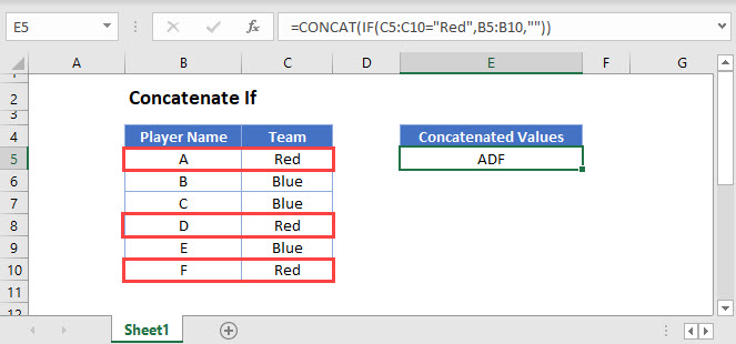
This example will use the CONCAT and IF Functions in an array formula to create a text string of Player Names which relate to a Team value of Red

=CONCAT(IF(C3:C8="Red",B3:B8,""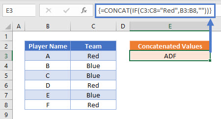

Users of Excel 2019 will need to enter this formula as an array function by pressing CTRL + SHIFT + ENTER. Users of later versions of Excel do not need to follow this step.

To explain what this formula is doing, lets break it down into steps:

This is our final formula:

=CONCAT(IF(C3:C8="Red",B3:B8,""

First, Excel reads the range values into the formula:

=CONCAT(IF({"Red"; "Blue"; "Blue"; "Red"; "Blue"; "Red"}="Red",{"A"; "B"; "C"; "D"; "E"; "F"},""

Next the list of Team names is compared to the value Red:

=CONCAT(IF({TRUE; FALSE; FALSE; TRUE; FALSE; TRUE},{"A"; "B"; "C"; "D"; "E"; "F"},""

The IF Function replaces TRUE values with the Player Name, and FALSE values with “”

=CONCAT({"A"; ""; ""; "D"; ""; "F"

The CONCAT Function then combines all of the array values into one text string:

="ADF"

Adding Delimiters or Ignoring Empty Values

If it is required to add delimiting values or text between each value, or for the function to ignore empty cell values, The TEXTJOIN Function can be used instead if you need to add delimiters

Read our TEXTJOIN If article to learn more.

Concatenate If – in pre-Excel 2019

As the CONCAT and TEXTJOIN Functions are not available before the Excel 2019 version, we need to solve this problem in a different way. The CONCATENATE Function is available but does not take ranges of cells as inputs or allow array operations and so we are required to use a helper column with an IF Function instead.

This next example shows how to use a helper column to create a text string of Player Names which relate to a Team value of Red:

=IF(C3="Red",B3,"" &D4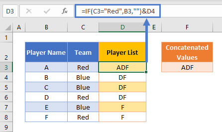

The first step in this example is to use an IF Function to replicate the condition of Team = Red:

=IF(C3="Red",B3,""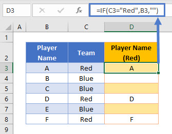

Next, we can create a column that builds up a list of these values into one cell by also referencing the cell below it:

=D3&E4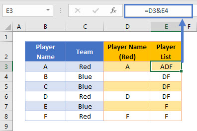

This formula uses the & character to join two values together. Note that the CONCATENATE Function could be used to create exactly the same result, but the & method is often preferred as it is shorter and makes it clearer what action the formula is performing.

These two helper columns can then be combined into one formula:

=IF(C3="Red",B3,""&D4

A summary cell can then reference the first value in the Player List helper column:

=D3

Concatenate If in Google Sheets

Google Sheets users should use the TEXTJOIN Function to concatenate values based on a condition.

This example will use the TEXTJOIN and IF Functions to create a text string of Player Names which relate to a Team value of Red

=ARRAYFORMULA(TEXTJOIN("",FALSE,IF(C3:C8="Red",B3:B8,"")))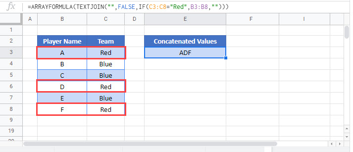

As this formula requires array inputs for the cell ranges, the ARRAYFORMULA Function should be added to the formula by pressing CTRL + SHIFT + ENTER.

Склеивание текста по условию

Про то, как можно быстро склеивать текст из нескольких ячеек в одну и, наоборот, разбирать длинную текстовую строку на составляющие я уже писал. Теперь же давайте рассмотрим близкую, но чуть более сложную задачу — как склеивать текст из нескольких ячеек при выполнении определенного заданного условия. 

Допустим, что у нас имеется база данных по клиентам, где одному названию компании может соответствовать несколько разных email’ов ее сотрудников. Наша задача состоит в том, чтобы собрать все адреса по названиям компаний и сцепить их (через запятую или точку с запятой), чтобы сделать потом, например, почтовую рассылку по клиентам, т.е. получить на выходе что-то похожее на:

Другими словами, нам нужен инструмент, который будет склеивать (сцеплять) текст по условию — аналог функции СУММЕСЛИ (SUMIF), но для текста.

Способ 0. Формулой

Не очень изящный, зато самый простой способ. Можно написать несложную формулу, которая будет проверять отличается ли компания в очередной строке от предыдущей.  Если не отличается, то приклеиваем через запятую очередной адрес. Если отличается, то «сбрасываем» накопленное, начиная заново:

Минусы такого подхода очевидны: из всех ячеек полученного дополнительного столбца нам нужны только последние по каждой компании (желтые). Если список большой, то чтобы их быстро отобрать придется добавить еще один столбец, использующий функцию ДЛСТР (LEN), проверяющий длину накопленных строк:

Теперь можно отфильтровать единички и скопировать нужные склейки адресов для дальнейшего использования.

Способ 1. Макрофункция склейки по одному условию

Если исходный список не отсортирован по компаниям, то приведенная выше простая формула не работает, но можно легко выкрутиться с помощью небольшой пользовательской функции на VBA. Откройте редактор Visual Basic нажатием на сочетание клавиш Alt+F11 или с помощью кнопки Visual Basic на вкладке Разработчик (Developer). В открывшемся окне вставьте новый пустой модуль через меню Insert — Module и скопируйте туда текст нашей функции:

Function MergeIf(TextRange As Range, SearchRange As Range, Condition As String)
    Dim Delimeter As String, i As Long
    Delimeter = ", " 'символы-разделители (можно заменить на пробел или ; и т.д.)
    
    'если диапазоны проверки и склеивания не равны друг другу - выходим с ошибкой
    If SearchRange.Count <> TextRange.Count Then
        MergeIf = CVErr(xlErrRef)
        Exit Function
    End If
    
    'проходим по все ячейкам, проверяем условие и собираем текст в переменную OutText
    For i = 1 To SearchRange.Cells.Count
        If SearchRange.Cells(i) Like Condition Then OutText = OutText & TextRange.Cells(i) & Delimeter
    Next i
    
    'выводим результаты без последнего разделителя
    MergeIf = Left(OutText, Len(OutText) - Len(Delimeter))
End Function

Если теперь вернуться в Microsoft Excel, то в списке функций (кнопка fx в строке формул или вкладка Формулы — Вставить функцию) можно будет найти нашу функцию MergeIf в категории Определенные пользователем (User Defined). Аргументы у функции следующие:

Способ 2. Сцепить текст по неточному условию

Если заменить в 13-й строчке нашего макроса первый знак = на оператор приблизительного совпадения Like, то можно будет осуществлять склейку по неточному совпадению исходных данных с критерием отбора. Например, если название компании может быть записано в разных вариантах, то мы можем одной функцией проверить и собрать их все:

Поддерживаются стандартные спецсимволы подстановки:

• звездочка (*) — обозначает любое количество любых символов (в т.ч. и их отсутствие)
• вопросительный знак (?) — обозначает один любой символ
• решетка (#) — обозначает одну любую цифру (0-9)

По умолчанию оператор Like регистрочувствительный, т.е. понимает, например, «Орион» и «оРиОн» как разные компании. Чтобы не учитывать регистр можно добавить в самое начало модуля в редакторе Visual Basic строчку Option Compare Text, которая переключит Like в режим, когда он невосприимчив к регистру.

Таким образом можно составлять весьма сложные маски для проверки условий, например:

• ?1##??777RUS — выборка по всем автомобильным номерам 777 региона, начинающимся с 1
• ООО* — все компании, название которых начинается на ООО
• ##7## — все товары с пятизначным цифровым кодом, где третья цифра 7
• ????? — все названия из пяти букв и т.д.

Способ 3. Макрофункция склейки текста по двум условиям

В работе может встретиться задача, когда сцеплять текст нужно больше, чем по одному условию. Например представим, что в нашей предыдущей таблице добавился еще один столбец с городом и склеивание нужно проводить не только для заданной компании, но еще и для заданного города. В этом случае нашу функцию придется немного модернизировать, добавив к ней проверку еще одного диапазона:

Function MergeIfs(TextRange As Range, SearchRange1 As Range, Condition1 As String, SearchRange2 As Range, Condition2 As String)
    Dim Delimeter As String, i As Long
    Delimeter = ", " 'символы-разделители (можно заменить на пробел или ; и т.д.)
    
    'если диапазоны проверки и склеивания не равны друг другу - выходим с ошибкой
    If SearchRange1.Count <> TextRange.Count Or SearchRange2.Count <> TextRange.Count Then
        MergeIfs = CVErr(xlErrRef)
        Exit Function
    End If
    
    'проходим по все ячейкам, проверяем все условия и собираем текст в переменную OutText
    For i = 1 To SearchRange1.Cells.Count
        If SearchRange1.Cells(i) = Condition1 And SearchRange2.Cells(i) = Condition2 Then
            OutText = OutText & TextRange.Cells(i) & Delimeter
        End If
    Next i
    
    'выводим результаты без последнего разделителя
    MergeIfs = Left(OutText, Len(OutText) - Len(Delimeter))
End Function

Применяться она будет совершенно аналогично — только аргументов теперь нужно указывать больше:

Способ 4. Группировка и склейка в Power Query

Решить проблему можно и без программирования на VBA, если использовать бесплатную надстройку Power Query. Для Excel 2010-2013 ее можно скачать здесь, а в Excel 2016 она уже встроена по умолчанию. Последовательность действий будет следующей:

Power Query не умеет работать с обычными таблицами, поэтому первым шагом превратим нашу таблицу в «умную». Для этого ее нужно выделить и нажать сочетание Ctrl+T или выбрать на вкладке Главная — Форматировать как таблицу (Home — Format as Table). На появившейся затем вкладке Конструктор (Design) можно задать имя таблицы (я оставил стандартное Таблица1):

Теперь загрузим нашу таблицу в надстройку Power Query. Для этого на вкладке Данные (если у вас Excel 2016) или на вкладке Power Query (если у вас Excel 2010-2013) жмем Из таблицы (Data — From Table):

В открывшемся окне редактора запросов выделяем щелчком по заголовку столбец Компания и сверху жмем кнопку Группировать (Group By). Вводим имя нового столбца и тип операции в группировке — Все строки (All Rows):

Жмем ОК и получаем для каждой компании мини-таблицу сгруппированных значений. Содержимое таблиц хорошо видно, если щелкать левой кнопкой мыши в белый фон ячеек (не в текст!) в получившемся столбце:

Теперь добавим еще один столбец, где с помощью функции склеим через запятую содержимое столбцов Адрес в каждой из мини-таблиц. Для этого на вкладке Добавить столбец жмем Пользовательский столбец (Add column — Custom column) и в появившемся окне вводим имя нового столбца и формулу сцепки на встроенном в Power Query языке М:

Обратите внимание, что все М-функции регистрочувствительные (в отличие от Excel). После нажатия на ОК получаем новый столбец со склееными адресами:

Осталось удалить ненужный уже столбец ТаблАдресов (правой кнопкой мыши по заголовку — Удалить столбец) и выгрузить результаты на лист, нажав на вкладке Главная — Закрыть и загрузить (Home — Close and load):

Важный нюанс: в отличие от предыдущих способов (функций), таблицы из Power Query не обновляются автоматически. Если в будущем произойдут какие-либо изменения в исходных данных, то нужно будет щелкнуть правой кнопкой в любое место таблицы результатов и выбрать команду Обновить (Refresh).

Ссылки по теме

• Как разделить длинную текстовую строку на части
• Несколько способов склеить текст из разных ячеек в одной
• Использование оператора Like для проверки текста по маске