
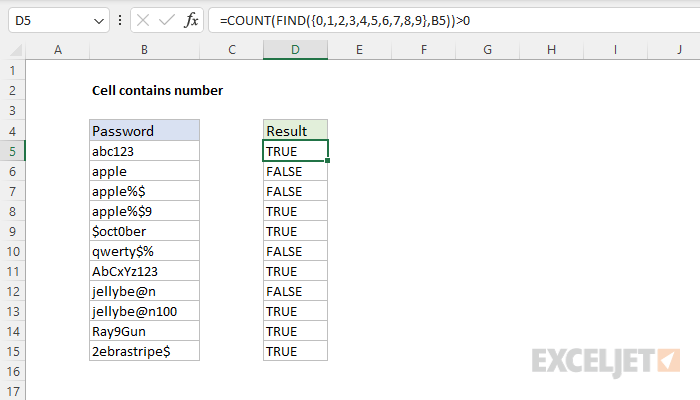
In this example, the goal is to test the passwords in column B to see if they contain a number. This is a surprisingly tricky problem because Excel doesn’t have a function that will let you test for a number inside a text string directly. Note this is different from checking if a cell value is a number. You can easily perform that test with the ISNUMBER function. In this case, however, we to test if a cell value contains a number, which may occur anywhere. One solution is to use the FIND function with an array constant. In Excel 365, which supports dynamic array formulas, you can use a different formula based on the SEQUENCE function. Both approaches are explained below.
FIND function
The FIND function is designed to look inside a text string for a specific substring. If FIND finds the substring, it returns a position of the substring in the text as a number. If the substring is not found, FIND returns a #VALUE error. For example:
=FIND("p","apple") // returns 2
=FIND("z","apple") // returns #VALUE!
We can use this same idea to check for numbers as well:
=FIND(3,"app637") // returns 5
=FIND(9,"app637") // returns #VALUE!
The challenge in this case is that we need to check the values in column B for ten different numbers, 0-9. One way to do that is to supply these numbers as the array constant {0,1,2,3,4,5,6,7,8,9}. This is the approach taken in the formula in cell D5:
=COUNT(FIND({0,1,2,3,4,5,6,7,8,9},B5))>0Inside the COUNT function, the FIND function is configured to look for all ten numbers in cell B5:
FIND({0,1,2,3,4,5,6,7,8,9},B5)Because we are giving FIND ten values to look for, it returns an array with 10 results. In other words, FIND checks the text in B5 for each number and returns all results at once:
{#VALUE!,4,5,6,#VALUE!,#VALUE!,#VALUE!,#VALUE!,#VALUE!,#VALUE!}Unless you look at arrays often, this may look pretty cryptic. Here is the translation: The number 1 was found at position 4, the number 2 was found at position 5, and the number 3 was found at position 6. All other numbers were not found and returned #VALUE errors.
We are very close now to a final formula. We simply need to tally up results. To do this, we nest the FIND formula above inside the COUNT function like this:
=COUNT(FIND({0,1,2,3,4,5,6,7,8,9},B5))FIND returns the array of results directly to COUNT, which counts the numbers in the array. COUNT only counts numeric values, and ignores errors. This means COUNT will return a number greater than zero if there are any numbers in the value being tested. In the case of cell B5, COUNT returns 3.
The last step is to check the result from COUNT and force a TRUE or FALSE result. We do this by adding «>0» to the end of formula:
=COUNT(FIND({0,1,2,3,4,5,6,7,8,9},B5))>0Now the formula will return TRUE or FALSE. To display a custom result, you can use the IF function:
=IF(COUNT(FIND({0,1,2,3,4,5,6,7,8,9},B5))>0, "Yes", "No")
The original formula is now nested inside IF as the logical_test argument. This formula will return «Yes» if B5 contains a number and «No» if not.
SEQUENCE function
In Excel 365, which offers dynamic array formulas, we can take a different approach to this problem.
=COUNT(--MID(B5,SEQUENCE(LEN(B5)),1))>0This isn’t necessarily a better approach, just a different way to solve the same problem. At the core, this formula uses the MID function together with the SEQUENCE function to split the text in cell B5 into an array:
MID(B5,SEQUENCE(LEN(B5)),1)Working from the inside out, the LEN function returns the length of the text in cell B5:
LEN(B5) // returns 6This number is returned to the SEQUENCE function as the rows argument, and SEQUENCE returns an array of numbers, 1-6:
=SEQUENCE(LEN(B5))
=SEQUENCE(6)
={1;2;3;4;5;6}
This array is returned to the MID function as the start_num argument, and, with num_chars set to 1, the MID function returns an array that contains the characters in cell B5:
=MID(B5,{1;2;3;4;5;6},1)
={"a";"b";"c";"1";"2";"3"}
We can now simplify the original formula to:
=COUNT(--{"a";"b";"c";"1";"2";"3"})>0We use the double-negative (—) to get Excel to try and coerce the values in the array into numbers. The result looks like this:
=COUNT({#VALUE!;#VALUE!;#VALUE!;1;2;3})>0The math operation created by the double negative (—) returns an actual number when successful and a #VALUE! error when the operation fails. The COUNT function counts the numbers, ignoring any errors, and returns 3. As above, we check the final count with «>0», and the result for cell B5 is TRUE.
Note: as you might guess, you can easily adapt this formula to count numbers in a text string.
Cell equals number?
Note that the formulas above are too complex if you only want to test if a cell equals a number. In that case, you can simply use the ISNUMBER function like this:
=ISNUMBER(A1)
This tutorial demonstrates how to check if a cell contains any number in Excel and Google Sheets.
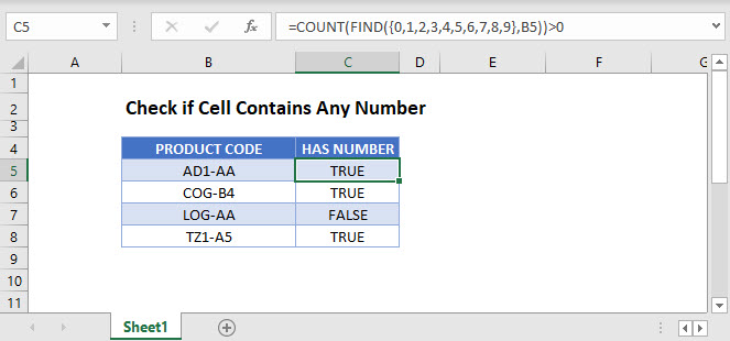
Cell Contains Any Number
In Excel, if a cell contains numbers and letters, the cell is considered a text cell. You can check if a text cell contains any number by using the COUNT and FIND Functions.
=COUNT(FIND({0,1,2,3,4,5,6,7,8,9},B3))>0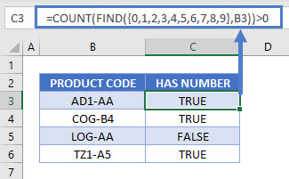
The formula above checks for the digits 0–9 in a cell and counts the number of discrete digits the cell contains. Then it returns TRUE if the count is positive or FALSE if it is zero.
Let’s step through each function below to understand this example.
FIND a Number in a Cell
First, we use the FIND Function. The FIND Function finds the position of a character within a text string.
=FIND({0,1,2,3,4,5,6,7,8,9},B3)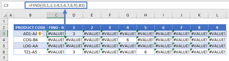
In this example, we use an array of all numerical characters (digits 0–9) and find each one in the cell. Since our input is an array – in curly brackets {} – our output is also an array. The example above shows how the FIND Function is performed ten times on each cell (once for each numerical digit).
If the number is found, it’s position is output. Above you can see the number “1” is found in the 3rd position in the first row and “4” is found in the 6th position in the 2nd row.
If a number is not found, the #VALUE! Error is displayed.
Note: The FIND and SEARCH Functions return the same result when used to search for numbers. Either function can be used.
COUNT the Number of Digits
Next, we count the non-error outputs from the last step. The COUNT Function counts the number of numeric values found in the array, ignoring errors.
=COUNT(C3:L3)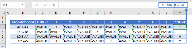
Test the Number Count
Finally, we need to test whether the result from the last step is greater than zero. The formula below returns TRUE for non-zero counts (where the target cell contains a number) and FALSE for any zero counts.
=M3>0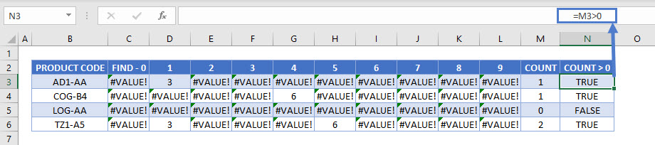
Combining these steps gives us our initial formula:
=COUNT(FIND({0,1,2,3,4,5,6,7,8,9},B3))>0
Check if Cell Contains Specific Number
To check if a cell contains a specific number, we can use the FIND or SEARCH Function.
=FIND(5,B3)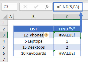
In this example we use the FIND Function to check for the number 5 in column B. It returns the position of the number 5 in the cell if it is found and a VALUE error if “5” is not found.
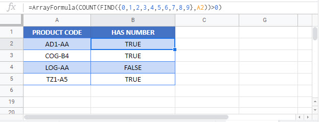
Check if Cell Contains Any Number – Google Sheets
These formulas work the same in Google Sheets as in Excel. However, you need to press CTRL + SHIFT + ENTER for Google Sheets to recognize an array formula.
Alternatively, you could type “ArrayFormula” and put the formula in parentheses. Both methods produce the same result.
Excel has a number of formulas that help you use your data in useful ways. For example, you can get an output based on whether or not a cell meets certain specifications. Right now, we’ll focus on a function called “if cell contains, then”. Let’s look at an example.
Jump To Specific Section:
- Explanation: If Cell Contains
- If cell contains any value, then return a value
- If cell contains text/number, then return a value
- If cell contains specific text, then return a value
- If cell contains specific text, then return a value (case-sensitive)
- If cell does not contain specific text, then return a value
- If cell contains one of many text strings, then return a value
- If cell contains several of many text strings, then return a value
Excel Formula: If cell contains
Generic formula
=IF(ISNUMBER(SEARCH("abc",A1)),A1,"")
Summary
To test for cells that contain certain text, you can use a formula that uses the IF function together with the SEARCH and ISNUMBER functions. In the example shown, the formula in C5 is:
=IF(ISNUMBER(SEARCH("abc",B5)),B5,"")
If you want to check whether or not the A1 cell contains the text “Example”, you can run a formula that will output “Yes” or “No” in the B1 cell. There are a number of different ways you can put these formulas to use. At the time of writing, Excel is able to return the following variations:
- If cell contains any value
- If cell contains text
- If cell contains number
- If cell contains specific text
- If cell contains certain text string
- If cell contains one of many text strings
- If cell contains several strings
Using these scenarios, you’re able to check if a cell contains text, value, and more.
Explanation: If Cell Contains
One limitation of the IF function is that it does not support Excel wildcards like «?» and «*». This simply means you can’t use IF by itself to test for text that may appear anywhere in a cell.
One solution is a formula that uses the IF function together with the SEARCH and ISNUMBER functions. For example, if you have a list of email addresses, and want to extract those that contain «ABC», the formula to use is this:
=IF(ISNUMBER(SEARCH("abc",B5)),B5,""). Assuming cells run to B5
If «abc» is found anywhere in a cell B5, IF will return that value. If not, IF will return an empty string («»). This formula’s logical test is this bit:
ISNUMBER(SEARCH("abc",B5))
Read article: Excel efficiency: 11 Excel Formulas To Increase Your Productivity
Using “if cell contains” formulas in Excel
The guides below were written using the latest Microsoft Excel 2019 for Windows 10. Some steps may vary if you’re using a different version or platform. Contact our experts if you need any further assistance.
1. If cell contains any value, then return a value
This scenario allows you to return values based on whether or not a cell contains any value at all. For example, we’ll be checking whether or not the A1 cell is blank or not, and then return a value depending on the result.
- Select the output cell, and use the following formula: =IF(cell<>»», value_to_return, «»).
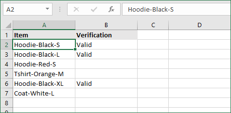
- For our example, the cell we want to check is A2, and the return value will be No. In this scenario, you’d change the formula to =IF(A2<>»», «No», «»).
- Since the A2 cell isn’t blank, the formula will return “No” in the output cell. If the cell you’re checking is blank, the output cell will also remain blank.
2. If cell contains text/number, then return a value
With the formula below, you can return a specific value if the target cell contains any text or number. The formula will ignore the opposite data types.
Check for text
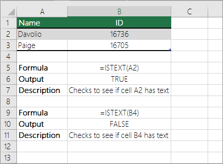
- To check if a cell contains text, select the output cell, and use the following formula: =IF(ISTEXT(cell), value_to_return, «»).
- For our example, the cell we want to check is A2, and the return value will be Yes. In this scenario, you’d change the formula to =IF(ISTEXT(A2), «Yes», «»).

- Because the A2 cell does contain text and not a number or date, the formula will return “Yes” into the output cell.
Check for a number or date
- To check if a cell contains a number or date, select the output cell, and use the following formula: =IF(ISNUMBER(cell), value_to_return, «»).
- For our example, the cell we want to check is D2, and the return value will be Yes. In this scenario, you’d change the formula to =IF(ISNUMBER(D2), «Yes», «»).

- Because the D2 cell does contain a number and not text, the formula will return “Yes” into the output cell.
3. If cell contains specific text, then return a value
To find a cell that contains specific text, use the formula below.
- Select the output cell, and use the following formula: =IF(cell=»text», value_to_return, «»).
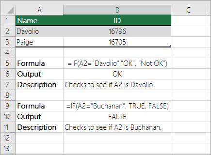
- For our example, the cell we want to check is A2, the text we’re looking for is “example”, and the return value will be Yes. In this scenario, you’d change the formula to =IF(A2=»example», «Yes», «»).

- Because the A2 cell does consist of the text “example”, the formula will return “Yes” into the output cell.
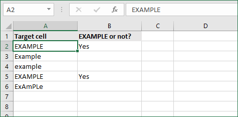
4. If cell contains specific text, then return a value (case-sensitive)
To find a cell that contains specific text, use the formula below. This version is case-sensitive, meaning that only cells with an exact match will return the specified value.
- Select the output cell, and use the following formula: =IF(EXACT(cell,»case_sensitive_text»), «value_to_return», «»).
- For our example, the cell we want to check is A2, the text we’re looking for is “EXAMPLE”, and the return value will be Yes. In this scenario, you’d change the formula to =IF(EXACT(A2,»EXAMPLE»), «Yes», «»).
- Because the A2 cell does consist of the text “EXAMPLE” with the matching case, the formula will return “Yes” into the output cell.
5. If cell does not contain specific text, then return a value
The opposite version of the previous section. If you want to find cells that don’t contain a specific text, use this formula.
- Select the output cell, and use the following formula: =IF(cell=»text», «», «value_to_return»).
- For our example, the cell we want to check is A2, the text we’re looking for is “example”, and the return value will be No. In this scenario, you’d change the formula to =IF(A2=»example», «», «No»).
- Because the A2 cell does consist of the text “example”, the formula will return a blank cell. On the other hand, other cells return “No” into the output cell.
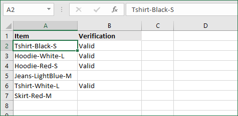
6. If cell contains one of many text strings, then return a value
This formula should be used if you’re looking to identify cells that contain at least one of many words you’re searching for.
- Select the output cell, and use the following formula: =IF(OR(ISNUMBER(SEARCH(«string1», cell)), ISNUMBER(SEARCH(«string2», cell))), value_to_return, «»).
- For our example, the cell we want to check is A2. We’re looking for either “tshirt” or “hoodie”, and the return value will be Valid. In this scenario, you’d change the formula to =IF(OR(ISNUMBER(SEARCH(«tshirt»,A2)),ISNUMBER(SEARCH(«hoodie»,A2))),»Valid «,»»).
- Because the A2 cell does contain one of the text values we searched for, the formula will return “Valid” into the output cell.
To extend the formula to more search terms, simply modify it by adding more strings using ISNUMBER(SEARCH(«string», cell)).
7. If cell contains several of many text strings, then return a value
This formula should be used if you’re looking to identify cells that contain several of the many words you’re searching for. For example, if you’re searching for two terms, the cell needs to contain both of them in order to be validated.
- Select the output cell, and use the following formula: =IF(AND(ISNUMBER(SEARCH(«string1»,cell)), ISNUMBER(SEARCH(«string2″,cell))), value_to_return,»»).
- For our example, the cell we want to check is A2. We’re looking for “hoodie” and “black”, and the return value will be Valid. In this scenario, you’d change the formula to =IF(AND(ISNUMBER(SEARCH(«hoodie»,A2)),ISNUMBER(SEARCH(«black»,A2))),»Valid «,»»).
- Because the A2 cell does contain both of the text values we searched for, the formula will return “Valid” to the output cell.
Final thoughts
We hope this article was useful to you in learning how to use “if cell contains” formulas in Microsoft Excel. Now, you can check if any cells contain values, text, numbers, and more. This allows you to navigate, manipulate and analyze your data efficiently.
We’re glad you’re read the article up to here  Thank you
You may also like
» How to use NPER Function in Excel
» How to Separate First and Last Name in Excel
» How to Calculate Break-Even Analysis in Excel
Содержание
- Check if a cell contains text (case-insensitive)
- Find cells that contain text
- Check if a cell has any text in it
- Check if a cell matches specific text
- Check if part of a cell matches specific text
- Check if Cell Contains Any Number – Excel & Google Sheets
- Cell Contains Any Number
- FIND a Number in a Cell
- COUNT the Number of Digits
- Test the Number Count
- Check if Cell Contains Specific Number
- Check if Cell Contains Any Number – Google Sheets
- Cell contains number
- Related functions
- Summary
- Generic formula
- Explanation
- FIND function
- SEQUENCE function
- Cell equals number?
- Cell contains specific text
- Related functions
- Summary
- Generic formula
- Explanation
- SEARCH function (not case-sensitive)
- Wildcards
- FIND function (case-sensitive)
- If cell contains
- With hardcoded search string
Check if a cell contains text (case-insensitive)
Let’s say you want to ensure that a column contains text, not numbers. Or, perhapsyou want to find all orders that correspond to a specific salesperson. If you have no concern for upper- or lowercase text, there are several ways to check if a cell contains text.
You can also use a filter to find text. For more information, see Filter data.
Find cells that contain text
Follow these steps to locate cells containing specific text:
Select the range of cells that you want to search.
To search the entire worksheet, click any cell.
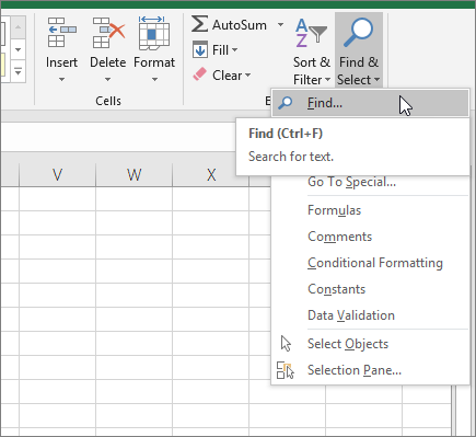
On the Home tab, in the Editing group, click Find & Select, and then click Find.
In the Find what box, enter the text—or numbers—that you need to find. Or, choose a recent search from the Find what drop-down box.
Note: You can use wildcard characters in your search criteria.
To specify a format for your search, click Format and make your selections in the Find Format popup window.
Click Options to further define your search. For example, you can search for all of the cells that contain the same kind of data, such as formulas.
In the Within box, you can select Sheet or Workbook to search a worksheet or an entire workbook.
Click Find All or Find Next.
Find All lists every occurrence of the item that you need to find, and allows you to make a cell active by selecting a specific occurrence. You can sort the results of a Find All search by clicking a header.
Note: To cancel a search in progress, press ESC.
Check if a cell has any text in it
To do this task, use the ISTEXT function.
Check if a cell matches specific text
Use the IF function to return results for the condition that you specify.
Check if part of a cell matches specific text
To do this task, use the IF, SEARCH, and ISNUMBER functions.
Note: The SEARCH function is case-insensitive.
Источник
Check if Cell Contains Any Number – Excel & Google Sheets
Download the example workbook
This tutorial demonstrates how to check if a cell contains any number in Excel and Google Sheets.
Cell Contains Any Number
In Excel, if a cell contains numbers and letters, the cell is considered a text cell. You can check if a text cell contains any number by using the COUNT and FIND Functions.
The formula above checks for the digits 0–9 in a cell and counts the number of discrete digits the cell contains. Then it returns TRUE if the count is positive or FALSE if it is zero.
Let’s step through each function below to understand this example.
FIND a Number in a Cell
First, we use the FIND Function. The FIND Function finds the position of a character within a text string.
In this example, we use an array of all numerical characters (digits 0–9) and find each one in the cell. Since our input is an array – in curly brackets <> – our output is also an array. The example above shows how the FIND Function is performed ten times on each cell (once for each numerical digit).
If the number is found, it’s position is output. Above you can see the number “1” is found in the 3rd position in the first row and “4” is found in the 6th position in the 2nd row.
If a number is not found, the #VALUE! Error is displayed.
Note: The FIND and SEARCH Functions return the same result when used to search for numbers. Either function can be used.
COUNT the Number of Digits
Next, we count the non-error outputs from the last step. The COUNT Function counts the number of numeric values found in the array, ignoring errors.
Test the Number Count
Finally, we need to test whether the result from the last step is greater than zero. The formula below returns TRUE for non-zero counts (where the target cell contains a number) and FALSE for any zero counts.
Combining these steps gives us our initial formula:
Check if Cell Contains Specific Number
To check if a cell contains a specific number, we can use the FIND or SEARCH Function.
In this example we use the FIND Function to check for the number 5 in column B. It returns the position of the number 5 in the cell if it is found and a VALUE error if “5” is not found.
Check if Cell Contains Any Number – Google Sheets
These formulas work the same in Google Sheets as in Excel. However, you need to press CTRL + SHIFT + ENTER for Google Sheets to recognize an array formula.
Alternatively, you could type “ArrayFormula” and put the formula in parentheses. Both methods produce the same result.
Источник
Cell contains number
Summary
To test if a cell or text string contains a number, you can use the FIND function together with the COUNT function. The numbers to look for are supplied as an array constant. In the example the formula in D5 is:
As the formula is copied down, it returns TRUE if a value contains a number and FALSE if not. See below for an alternate formula based on the SEQUENCE function.
Generic formula
Explanation
In this example, the goal is to test the passwords in column B to see if they contain a number. This is a surprisingly tricky problem because Excel doesn’t have a function that will let you test for a number inside a text string directly. Note this is different from checking if a cell value is a number. You can easily perform that test with the ISNUMBER function. In this case, however, we to test if a cell value contains a number, which may occur anywhere. One solution is to use the FIND function with an array constant. In Excel 365, which supports dynamic array formulas, you can use a different formula based on the SEQUENCE function. Both approaches are explained below.
FIND function
The FIND function is designed to look inside a text string for a specific substring. If FIND finds the substring, it returns a position of the substring in the text as a number. If the substring is not found, FIND returns a #VALUE error. For example:
We can use this same idea to check for numbers as well:
The challenge in this case is that we need to check the values in column B for ten different numbers, 0-9. One way to do that is to supply these numbers as the array constant <0,1,2,3,4,5,6,7,8,9>. This is the approach taken in the formula in cell D5:
Inside the COUNT function, the FIND function is configured to look for all ten numbers in cell B5:
Because we are giving FIND ten values to look for, it returns an array with 10 results. In other words, FIND checks the text in B5 for each number and returns all results at once:
Unless you look at arrays often, this may look pretty cryptic. Here is the translation: The number 1 was found at position 4, the number 2 was found at position 5, and the number 3 was found at position 6. All other numbers were not found and returned #VALUE errors.
We are very close now to a final formula. We simply need to tally up results. To do this, we nest the FIND formula above inside the COUNT function like this:
FIND returns the array of results directly to COUNT, which counts the numbers in the array. COUNT only counts numeric values, and ignores errors. This means COUNT will return a number greater than zero if there are any numbers in the value being tested. In the case of cell B5, COUNT returns 3.
The last step is to check the result from COUNT and force a TRUE or FALSE result. We do this by adding «>0» to the end of formula:
Now the formula will return TRUE or FALSE. To display a custom result, you can use the IF function:
The original formula is now nested inside IF as the logical_test argument. This formula will return «Yes» if B5 contains a number and «No» if not.
SEQUENCE function
In Excel 365, which offers dynamic array formulas, we can take a different approach to this problem.
This isn’t necessarily a better approach, just a different way to solve the same problem. At the core, this formula uses the MID function together with the SEQUENCE function to split the text in cell B5 into an array:
Working from the inside out, the LEN function returns the length of the text in cell B5:
This number is returned to the SEQUENCE function as the rows argument, and SEQUENCE returns an array of numbers, 1-6:
This array is returned to the MID function as the start_num argument, and, with num_chars set to 1, the MID function returns an array that contains the characters in cell B5:
We can now simplify the original formula to:
We use the double-negative (—) to get Excel to try and coerce the values in the array into numbers. The result looks like this:
The math operation created by the double negative (—) returns an actual number when successful and a #VALUE! error when the operation fails. The COUNT function counts the numbers, ignoring any errors, and returns 3. As above, we check the final count with «>0», and the result for cell B5 is TRUE.
Note: as you might guess, you can easily adapt this formula to count numbers in a text string.
Cell equals number?
Note that the formulas above are too complex if you only want to test if a cell equals a number. In that case, you can simply use the ISNUMBER function like this:
Источник
Cell contains specific text
Summary
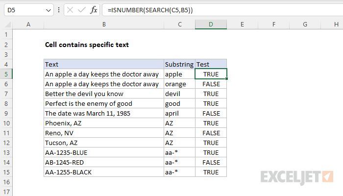
To check if a cell contains specific text (i.e. a substring), you can use the SEARCH function together with the ISNUMBER function. In the example shown, the formula in D5 is:
This formula returns TRUE if the substring is found, and FALSE if not. Note the SEARCH function is not case-sensitive. See below for a case-sensitive formula.
Generic formula
Explanation
In this example, the goal is to test a value in a cell to see if it contains a specific substring. Excel contains two functions designed to check the occurrence of one text string inside another: the SEARCH function and the FIND function. Both functions return the position of the substring if found as a number, and a #VALUE! error if the substring is not found. The difference is that the SEARCH function supports wildcards but is not case-sensitive, while the FIND function is case-sensitive but does not support wildcards. The general approach with either function is to use the ISNUMBER function to check for a numeric result (a match) and return TRUE or FALSE.
SEARCH function (not case-sensitive)
The SEARCH function is designed to look inside a text string for a specific substring. If SEARCH finds the substring, it returns a position of the substring in the text as a number. If the substring is not found, SEARCH returns a #VALUE error. For example:
To force a TRUE or FALSE result, we use the ISNUMBER function. ISNUMBER returns TRUE for numeric values and FALSE for anything else. So, if SEARCH finds the substring, it returns the position as a number, and ISNUMBER returns TRUE:
If SEARCH doesn’t find the substring, it returns an error, which causes the ISNUMBER to return FALSE.
Wildcards
Although SEARCH is not case-sensitive, it does support wildcards (*?
). For example, the question mark (?) wildcard matches any one character. The formula below looks for a 3-character substring beginning with «x» and ending in «y»:
The asterisk (*) wildcard matches zero or more characters. This wildcard is not as useful in the SEARCH function because SEARCH already looks for a substring. For example, it might seem like the following formula will test for a value that ends with «z»:
However, because SEARCH automatically looks for a substring, the following formulas all return 1 as a result, even though the text in the first formula is the only text that ends with «z»:
This means the asterisk (*) is not a reliable way to test for «ends with». However, you an use the the asterisk (*) wildcard like this:
Here we are looking for «x», «2», and «b» in that order, with any number of characters in between. Finally, you can use the tilde (
) as an escape character to indicate that the next character is a literal like this:
The above formulas use SEARCH to find a literal asterisk (*), question mark (?) , and tilde (
FIND function (case-sensitive)
Like the SEARCH function, the FIND function returns the position of a substring in text as a number, and an error if the substring is not found. However, unlike the SEARCH function, the FIND function respects case:
To make a case-sensitive version of the formula, just replace the SEARCH function with the FIND function in the formula above:
The result is a case-sensitive search:
If cell contains
To return a custom result when a cell contains specific text, add the IF function like this:
Instead of returning TRUE or FALSE, the formula above will return «Yes» if substring is found and «No» if not.
With hardcoded search string
To test for a hardcoded substring, enclose the text in double quotes («»). For example, to check A1 for the text «apple» use:
Источник
EXPLANATION
tutorial shows how to test if a range contains a cell with a number and return a specified value if the formula tests true or false, by using an Excel formula and VBA.
This tutorial provides one Excel method that can be applied to test if a range contains at least one cell that has only numbers by using a combination of Excel IF, SUMPRODUCT and ISNUMBER functions. In this example, if the SUMPRODUCT and ISNUMBER part of the formula returns a value of greater than 0, meaning the range contains cells that only captures number, the test is TRUE and the formula will return a «Contains Number» value. Alternatively, if the SUMPRODUCT and ISNUMBER part of the formula returns a value of 0, meaning the range does not have any cells that only capture numbers, the test is FALSE and the formula will return a «No Number» value.
This tutorial provides one VBA method that can be applied to test if a range contains at least one cell that has only numbers by looping through each cell in a selected range and using the IsNumeric function to identify if a cell contains only numbers. As soon as the it identifies the first cell that contains only numbers it will return a value of «Contains Number» and exit loop. If the range does not contain any cells that contain only numbers, after looping through each cell in a range, it will return a value «No Number».
FORMULA
=IF(SUMPRODUCT(—ISNUMBER(range))>0,value_if_true, value_if_false)
ARGUMENTS
range: The range of cells you want to test if they contain only numeric values.
value_if_true: Value to be returned if the range contains at least one cell that has only numbers.
value_if_false: Value to be returned if the range does not contain any cells that contain only numbers.