Excel if cells are different

When you’re working with data in Excel, sooner or later you will have to compare data. This could be comparing two columns or even data in different sheets/workbooks.

In this Excel tutorial, I will show you different methods to compare two columns in Excel and look for matches or differences.

There are multiple ways to do this in Excel and in this tutorial I will show you some of these (such as comparing using VLOOKUP formula or IF formula or Conditional formatting).

So let’s get started!

Compare Two Columns (Side by Side)

This is the most basic type of comparison where you need to compare a cell in one column with the cell in the same row in another column.

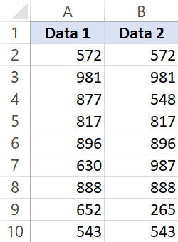
Suppose you have a dataset as shown below and you simply want to check whether the value in column A in a specific cell is the same (or different) when compared with the value in the adjacent cell.

Of course, you can do this when you have a small dataset when you have a large one, you can use a simple comparison formula to get this done. And remember, there is always a chance of human error when you do this manually.

So let me show you a couple of easy ways to do this.

Compare Side by Side Using the Equal to Sign Operator

Suppose you have the below dataset and you want to know what rows have the matching data and what rows have different data.

Below is a simple formula to compare two columns (side by side):

=A2=B2

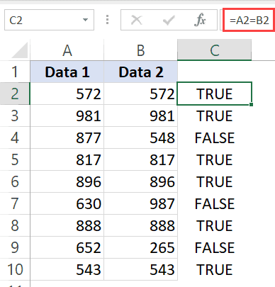
The above formula will give you a TRUE if both the values are the same and FALSE in case they are not.

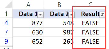
Now, if you need to know all the values that match, simply apply a filter and only show all the TRUE values. And if you want to know all the values that are different, filter all the values that are FALSE (as shown below):

When using this method to do column comparison in Excel, it’s always best to check that your data does not have any leading or trailing spaces. If these are present, despite having the same value, Excel will show them as different. Here is a great guide on how to remove leading and trailing spaces in Excel.

Compare Side by Side Using the IF Function

Another method that you can use to compare two columns can be by using the IF function.

This is similar to the method above where we used the equal to (=) operator, with one added advantage. When using the IF function, you can choose the value you want to get when there are matches or differences.

For example, if there is a match, you can get the text “Match” or can get a value such as 1. Similarly, when there is a mismatch, you can program the formula to give you the text “Mismatch” or give you a 0 or blank cell.

Below is the IF formula that returns ‘Match’ when the two cells have the cell value and ‘Not a Match’ when the value is different.

=IF(A2=B2,"Match","Not a Match")

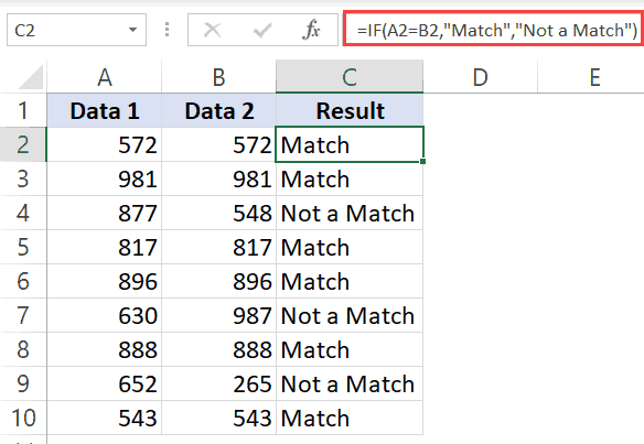
The above formula uses the same condition to check whether the two cells (in the same row) have matching data or not (A2=B2). But since we are using the IF function, we can ask it to return a specific text in case the condition is True or False.

Once you have the formula results in a separate column, you can quickly filter the data and get rows that have the matching data or rows with mismatched data.

Also read: Does Not Equal Operator in Excel (Examples)

Highlight Rows with Matching Data (or Different Data)

Another great way to quickly check the rows that have matching data (or have different data), is to highlight these rows using conditional formatting.

You can do both – highlight rows that have the same value in a row as well as the case when the value is different.

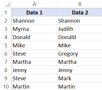
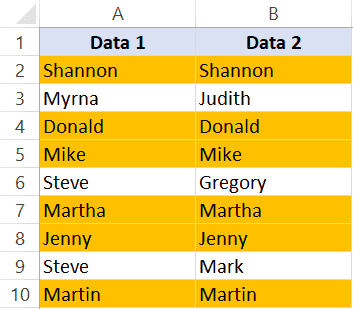
Suppose you have a dataset as shown below and you want to highlight all the rows where the name is the same.

Below are the steps to use conditional formatting to highlight rows with matching data:

1. Select the entire dataset (except the headers)
2. Click the Home tab
3. In the Styles group, click on Conditional Formatting
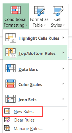
4. In the options that show up, click on ‘New Rule’
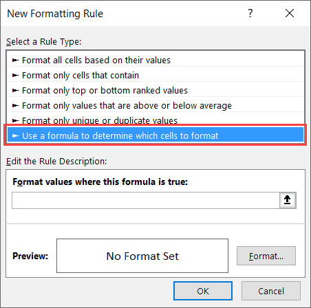
5. In the ‘New Formatting Rule’ dialog box, click on the option -”Use a formula to determine which cells to format’
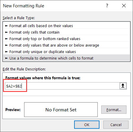
6. In the ‘Format values where this formula is true’ field, enter the formula: =$A2=$B2
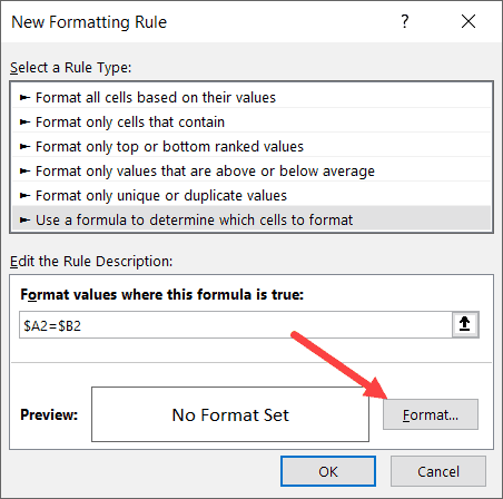
7. Click on the Format button
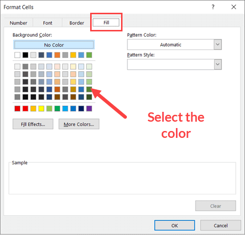
8. Click on the ‘Fill’ tab and select the color in which you want to highlight the rows with the same value in both columns
9. Click OK

The above steps would instantly highlight the rows where the name is the same in both columns A and B (in the same row). And in the case where the name is different, those rows will not be highlighted.

In case you want to compare two columns and highlight rows where the names are different, use the below formula in the conditional formatting dialog box (in step 6).

=$A2<>$B2

How does this work?

When we use conditional formatting with a formula, it only highlights those cells where the formula is true.

When we use $A2=$B2, it will check each cell (in both columns) and see whether the value in a row in column A is equal to the one in column B or not.

In case it’s an exact match, it will highlight it in the specified color, and in case it doesn’t match, it will not.

The best part about conditional formatting is that it doesn’t require you to use a formula in a separate column. Also, when you apply the rule on a dataset, it remains dynamic. This means that if you change any name in the dataset, conditional formatting will accordingly adjust.

Compare Two Columns Using VLOOKUP (Find Matching/Different Data)

In the above examples, I showed you how to compare two columns (or lists) when we are just comparing side by side cells.

In reality, this is rarely going to be the case.

In most cases, you will have two columns with data and you would have to find out whether a data point in one column exists in the other column or not.

In such cases, you can’t use a simple equal-to sign or even an IF function.

You need something more powerful…

… something that’s right up VLOOKUP’s alley!

Let me show you two examples where we compare two columns in Excel using the VLOOKUP function to find matches and differences.

Compare Two Columns Using VLOOKUP and Find Matches

Suppose we have a dataset as shown below where we have some names in columns A and B.

If you have to find out what are the names that are in column B that are also in column A, you can use the below VLOOKUP formula:

=IFERROR(VLOOKUP(B2,$A$2:$A$10,1,0),"No Match")

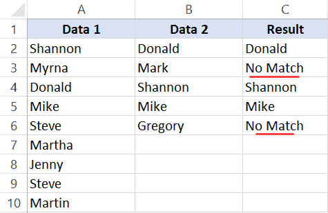
The above formula compares the two columns (A and B) and gives you the name in case the name is in column B as well A, and it returns “No Match” in case the name is in Column B and not in Column A.

By default, the VLOOKUP function will return a #N/A error in case it doesn’t find an exact match. So to avoid getting the error, I have wrapped the VLOOKUP function in the IFERROR function, so that it gives “No Match” when the name is not available in column A.

You can also do the other way round comparison – to check whether the name is in Column A as well as Column B. The below formula would do that:

=IFERROR(VLOOKUP(A2,$B$2:$B$6,1,0),"No Match")

Compare Two Columns Using VLOOKUP and Find Differences (Missing Data Points)

While in the above example, we checked whether the data in one column was there in another column or not.

You can also use the same concept to compare two columns using the VLOOKUP function and find missing data.

Suppose we have a dataset as shown below where we have some names in columns A and B.

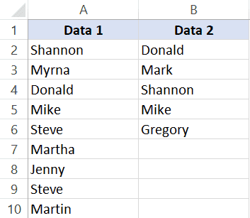
If you have to find out what are the names that are in column B that not there in column A, you can use the below VLOOKUP formula:

=IF(ISERROR(VLOOKUP(B2,$A$2:$A$10,1,0)),"Not Available","Available")

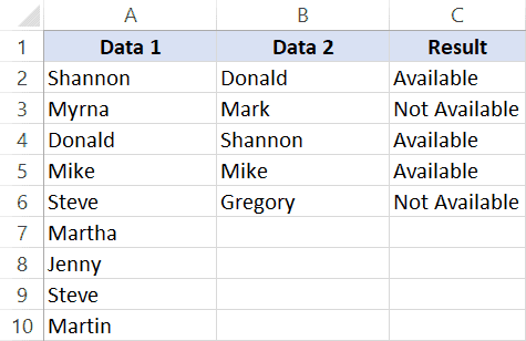
The above formula checks the name in column B against all the names in Column A. In case it finds an exact match, it would return that name, and in case it doesn’t find and exact match, it will return the #N/A error.

Since I am interested in finding the missing names that are there is column B and not in column A, I need to know the names that return the #N/A error.

This is why I have wrapped the VLOOKUP function in the IF and ISERROR functions. This whole formula gives the value – “Not Available” when the name is missing in Column A, and “Available” when it’s present.

To know all the names that are missing, you can filter the result column based on the “Not Available” value.

You can also use the below MATCH function to get the same result:

=IF(ISNUMBER(MATCH(B2,$A$2:$A$10,0)),"Available","Not Available")

Common Queries when Comparing Two Columns

Below are some common queries I usually get when people are trying to compare data in two columns in Excel.

Q1. How to compare multiple columns in Excel in the same row for matches? Count the total duplicates also.

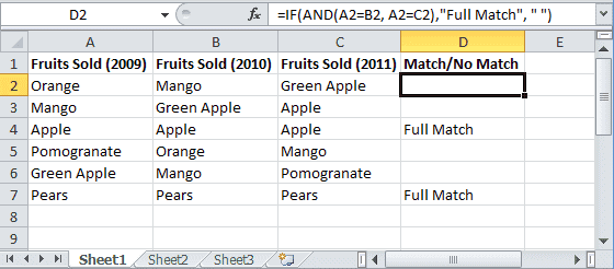
Ans. We have given the procedure to compare two columns in excel for the same row above. But if you want to compare multiple columns in excel for the same row then see the example

=IF(AND(A2=B2, A2=C2),"Full Match", "")

Here we have compared data of column A, column B, and column C. After this, I have applied the above formula in column D and get the result.

Now to count the duplicates, you need to use the Countif function.

=IF(COUNTIF($A2:$E2, $A2)=5, "Full Match", "")

Q2. Which operator do you use for matches and differences?

Ans. Below are the operators to use:

• To find matches, use the equal to sign (=)
• To find differences (mismatches), use the not-equal-to sign (<>)

Q3. How to compare two different tables and pull matching data?

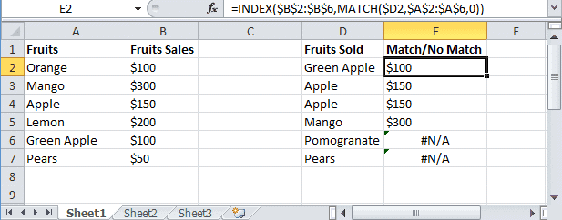
Ans. For this, you can use the VLOOKUP function or INDEX & MATCH function. To understand this thing in a better way we will take an example.

Here we will take two tables and now want to do pull matching data. In the first table, you have a dataset and in the second table, take the list of fruits and then use pull matching data in another column. For pull matching, use the formula

=INDEX($B$2:$B$6,MATCH($D2,$A$2:$A$6,0))

Q4. How to remove duplicates in Excel?

Ans. To remove duplicate data you need to first find the duplicate values.

To find the duplicate, you can use various methods like conditional formatting, Vlookup, If Statement, and many more. Excel also has an in-built tool where you can just select the data, and remove the duplicates from a column or even multiple columns

Q5. I can see that there is a matching value in both columns. However, the formulas you have shared above are not considering these as exact matches. Why?

Ans: Excel considers something an exact match when each and every character of one cell is equal to the other. There is a high chance that in your dataset there are leading or trailing spaces.

Although these spaces may still make the values seem equal to a naked eye, for Excel these are different. If you have such a dataset, it’s best to get rid of these spaces (you can use Excel functions such as TRIM for this).

Q7. How to compare two columns that give the result as TRUE when all first columns’ integer values are not less than the second column’s integer values. To solve this problem, I do not require conditional formatting, Vlookup function, If Statement, and any other formulas. I need the formula to solve this problem.

Ans. You can use the array formula for solving this problem.

The syntax is {=AND(H6:H12>I6:I12)}. This will give you “True” as a result whenever the value of Column H is greater than the value in column I else “False” will be the result.

You may also like the following Excel tutorials:

• Compare Two Columns in Excel (for matches and differences)
• How to Remove Blank Columns in Excel? (Formula + VBA)
• How to Hide Columns Based On Cell Value in Excel
• How to Split One Column into Multiple Columns in Excel
• How to Select Alternate Columns in Excel (or every Nth Column)
• How to Paste in a Filtered Column Skipping the Hidden Cells
• Best Excel Books (that will make you an Excel Pro)
• How to Flip Data in Excel (Columns, Rows, Tables)?
• Find the Closest Match in Excel (Nearest Value)
• How to Compare Two Cells in Excel?
• VLOOKUP Not Working – 7 Possible Reasons + How to Fix!

Aside from staring at them closely, how can you compare two cells in Excel? Here are a few functions and formulas that check the contents of two cells, to see if they are the same.

Easy Way to Compare Two Cells

To compare the two cells, we’ll start with a simple check, then try more complex comparisons.

• Tip: You can see more ways to compare two cells on my Contextures site. Get an Excel workbook with all the examples from that page too.

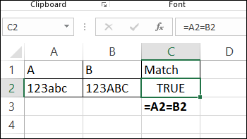
The quickest way to compare two cells is with a formula that uses the equal sign.

• =A2=B2

If the cell contents are the same, the result is TRUE. (Upper and lower case versions of the same letter are treated as equal).

Compare Two Cells Exactly

If you need to compare two cells for contents and upper/lower case, use the EXACT function. This video shows a few EXACT examples.

As its name indicate, the EXACT function can check for an exact match between text strings, including upper and lower case.

The EXACT function doesn’t test the formatting though, so it won’t detect if one cell has some or all of the characters in bold, and the other cell doesn’t.

• =EXACT(A2,B2)

See more EXACT function examples on my Contextures site.

Partially Compare Two Cells

Sometimes you don’t need a full comparison of two cells – you just need to check the first few characters, or a 3-digit code at the end of a string.

To compare characters at the beginning of the cells, use the LEFT function. For example, check the first 3 characters:

• =LEFT(A2,3)=LEFT(B2,3)

To compare characters at the end of the cells, use the RIGHT function. For example, check the last 3 characters, and combine with the EXACT function:

• =EXACT(RIGHT(A2,3),RIGHT(B2,3))

How Much Do Cells Match?

Finally, here’s a formula from UniMord, who needed to know how much of a match there is between two cells. What percent of the string in A2, starting from the left, is matched in cell B2?

Here’s a sample list, where three formulas check the addresses in column A and B, and calculate the percent that the characters match.

Get the Text Length

The first step in calculating the percent that the cells match is to find the length of the address in column A. This formula is in cell C2:

• =LEN(A2)

Get the Match Length

Next, the formula in column D  finds how many characters, starting from the left in each cell, are a match. Lower and upper case are not compared.

• =SUMPRODUCT(
  –(LEFT(A3,
  ROW(INDIRECT(“A1:A” & C3)))
  =LEFT(B3,
  ROW(INDIRECT(“A1:A” &C3)))))

Tip: If you’re using Excel 365, there’s a shorter formula you can use, with one of the new Spill functions. See the new formula on the Compare Two Cells page of my Contextures site.

How It Works

Here’s a quick overview of how the formula works, and there are detailed notes on the Compare Two Cells page of my Contextures site

1. INDIRECT and ROW functions create an array of numbers, from 1 to X
2. Left X characters from the two cells are compared, using equal sign
3. Comparison returns TRUE or FALSE
4. Two minus signs, near the start of the formula, converts TRUE and FALSE to ones and zeros
5. SUMPRODUCT function adds up numbers. In row 5, total is 1

Get the Percent Match

The final step is to find the percent matched, by dividing the two numbers:

• =D2/C2

There is a 100% match in row 2, and only a 20% match, starting from the left, in row 5.

Thanks, UniMord, for sharing your formula to compare two cells, character by character.

Get the Compare Cells Sample File

You download an Excel workbook with all the examples, and see more ways to compare two cells on my Contextures site. The sample workbook is in xlsx format, and does not contain any macros.

That page also has details on how the Percent Matched formulas work, and there’s a shorter version of the Percent Matched formula, if you’re using Excel 365.

More Ways to Compare Two Cells

Here are a few more articles that show examples of how to compare two cells – either the full content, or partial content.

• Use INDEX, MATCH and COUNTIF to find codes within text strings. There are other formulas in the comments too, so check those out.
• Compare formulas on different sheets, with the FORMULATEXT and INDIRECT functions. Those functions are volatile though, so they’d slow down the workbook if you use too many of them.
• Be careful when using the Remove Duplicates feature in Excel – it treats real numbers and text numbers as the same value

__________________________

___________________

How to Compare Two Columns in Excel: Step-by-Step

How to Compare Two Columns in Excel: Step-by-Step

Comparing two columns in Excel is something you’d need to do very often. Sometimes to see if both the columns tally. And the other times, to see if both the columns are unique to each other 👀

In both cases, Excel fails to offer any in-built feature to help you do that. Yeah, very unfortunate – but that’s how it is.

However, there are still many hacks that you can use to compare two columns in Excel.

To learn those, continue reading the guide below 👇

Also, download our free sample workbook here to tag along with the guide.

Compare two columns to find matches & differences

Comparing two columns to spot-matching data in Excel is all about putting an IF function in place 😎

For example, the image below has two lists.

Both lists contain names that apparently seem the same. But we still need to run a check to see if they are actually the same.

Oh no! Don’t start scanning the lists already. We have a hack to do that.

1. In a neighboring column to the lists (Column C), write the IF function as below:

= IF (

1. As the first argument, write in the logical test to be performed by the IF function.

= IF (A2=B2

We want to see if the first and the second list match. And so, we have set the logical test to be performed to Cell A2=B2. Excel would now check if Cell A2 is equal to B2 🚀

1. As the second argument, type in the value that you’d want to be returned if the logical test turns true (value_if_true).

You can set any value as the value_in_true enclosed in double quotation marks. For now, we are setting it to “Names match”.

= IF (A2=B2, “Names match”

1. For the value_if_false, type in the value that you’d want to be returned if the logical test turns false.

Let’s set it to “Names don’t match”.

= IF (A2=B2, “Names match”, ”Names don’t match”)

With this, we are all done writing the IF function 👍

1. Hit “Enter” to get the results as follows:

The result is “Names match” for the first row of the list. And we can clearly see the same name “Charles” in both lists.

1. Drag and drop the formula till the end (until the lists continue).

The whole list is now checked for the same data. And for some names (in Rows 3, 4, and 7), the IF function returns “Names don’t match” ❌

Pay attention to the dataset to note that for:

• Row 3: The spelling of “Tilbury” and “Tillbury” differs.
• Row 4: “Samia” and “Leon” are clearly two different names.
• Row 7: “Peter” and “Tim” are clearly two different names.

Kasper Langmann, Microsoft Office Specialist

This is one way how you can compare columns in Excel to know if both of the columns match or not. Such a row-to-row comparison also helps identify the individual items that differ (like Row 3,4, and 7 above) 🚴‍♀️

Compare two columns for case-sensitive matches

Take a quick look at the image below (Row 5).

The text “Pesso” in the first list starts with a capital P. Whereas, the text “pesso” in the second list starts with a small “p” 👆

However, the IF function treats them the same and returns the value “Names Match”.

This means that the IF function performs a case-insensitive comparison. But what if you want to run a case-sensitive comparison of two lists? Not a problem – we can do that too. See below.

1. Write the EXACT function as below:

= EXACT (A2,B2)

The EXACT function checks if two given cells (A2 and B2) have exactly the same value. It also checks for case sensitivity.

It returns TRUE if both the cells are equal, and FALSE if they are not exactly equal.

For the first row, the EXACT function returned TRUE. That’s because the name “Charles” in the first column is exactly the same as “Charles” in the second column.

1. Nest the EXACT function above in the IF function as follows.

= IF ( EXACT (A2,B2)

This will act as the logical test. If the EXACT function returns TRUE, the IF function will return the value_if_true.

And if the EXACT function returns FALSE, the IF function will return the value_if_false 🎯

1. Type in the value that you’d want to be returned if the EXACT function returns TRUE.

We are again setting it to “Names match”.

= IF ( EXACT (A2,B2), “Names match”

1. Type in the value that you’d want to be returned if the EXACT function returns FALSE.

= IF ( (EXACT(A2, B2), “Names match”, ”Names don’t match”)

1. Hit “Enter”.

1. Drag and drop the formula to the whole list.

Note that this time, the results for the same Row 5 (Pesso) change 🤩

The IF function now tells us that the names do not match because they do not have the same case.

Highlight matches or differences between two columns

If you don’t want a whole separate list of formulas and results while you compare two columns – no worries, we hear you.

Another efficient way to compare columns is by running conditional formatting in Excel. You can use it to identify matching and differing columns, both 🎨

Let’s see how.

1. Select the lists that you want to compare. If you don’t want both lists to be highlighted, you may select any one list only.

1. Go to Home Tab > Conditional Formatting.

1. From the drop-down list that appears, select Highlight Cell Rules option > More Rules.

This will take you to the “New Formatting Rule” dialog box as follows:

1. Under Rule Type, select “Use a formula to determine which cells to format”.
2. Under the Rule description, write the following formula:

=$A2=$B2

This tells Excel to format the cells where cell A2 is equal to cell B2.

We have turned the column reference into an absolute one so that the same formatting can be applied to the whole list 📝

Kasper Langmann, Microsoft Office Specialist

1. Click on the “Format” button to select any Format that you’d want to be applied to the cells of the list that match.

We have selected the Fill option in green color as below.

1. All done – Click “Okay”.

Excel highlights all the rows that match 📌

Pro Tip!

Did you note Row 5 (Pesso) being highlighted in green? This means conditional formatting also carries out a case-insensitive comparison of columns.

Similarly, if you want to apply conditional formatting to those rows of the lists that do not match:

1. Launch the “New Formatting Rule” dialog box.
2. Under Rule Type, select “Use a formula to determine which cells to format”.
3. Under the Rule description, write the following formula:

=$A2<>$B2

This tells Excel to format the cells where cell A2 is not equal to (<>) B2.

1. Choose any Format that you’d want to be applied to the cells that meet the above criterion. Like we are selecting a red fill.

1. Press “Enter” and you get the following results.

This time Excel has red-highlighted the cells that are different in the whole list ⭕

That’s it – Now what?

We hope you now know how to compare columns in Excel – whether to find matching items or unique items.

In the guide above, we’ve explored different functions that can help you do that. We also learned to use conditional formatting to highlight the similarities and differences between any two columns in Excel.

Excel functions and features are super versatile. Even if Excel misses out on a specific function, you can find a way to make that happen by tweaking some other Excel functions.

There are just so many functions in Excel to explore. And once you know them all – there’d be barely anything in Excel you couldn’t do 💪

Want to begin learning them? We suggest you start with the VLOOKUP function, SUMIF, and IF functions of Excel.

My 30-minute free email course teaches all details about these (and other) functions of Excel. Click here to sign up now.

Frequently asked questions

To check if two cells (say Cell A1 and B1) have the same text in Excel, apply the IF function as follows:

= IF (A1=B1, “Same Text”, “Not Same”)

If both the cells have duplicate values, the IF function would return “Same text”. And if there is some difference between both the cells, it will return “Not Same”.

To compare two lists (Say Column A and B) in Excel, apply the IF Function in a cell in Excel as follows:

= IF (A1=B1, “Same”, “Different”)

Drag and drop this formula to the whole list. The IF function will return “Same” for each row of the list that is the same in both columns and “Different” if it’s different.

Kasper Langmann2023-01-11T20:44:56+00:00

Bottom Line: Learn how to quickly check if there are values, formulas, or text in a row or column that are different from the other entries.

Skill Level: Beginner

Video Tutorial

Download the Excel File

If you’d like to download the same workbook that I use in the video, you can get it here:

Selecting Cells with Differences

This is a great tip for anyone who is auditing or reviewing a spreadsheet and wants to quickly find any abnormalities in the formulas or values that are being used for calculations.

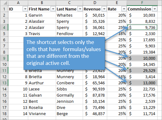
For example, in the spreadsheet that I use in the video, we want to quickly look for any cells where the sales commission is calculated differently from the norm.

You can easily select cells with differences or variations in formulas or values.

To do that, we start by highlighting the entries in a particular column that we want to check. Then we simply use the keyboard shortcut Ctrl + Shift + (backslash).

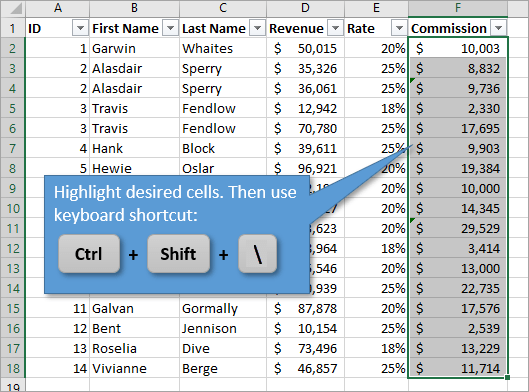
Note: The active cell in your highlighted column will be the basis for comparison. Using the keyboard shortcut will select all the abnormalities based on the formula in that active cell.

Flag or Highlight the Abnormal Cells

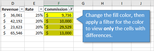
Once all of the cells with differences (exceptions or irregularities) are selected, we can then flag them for review.

With the abnormal cells selected, you can easily change the fill color for those cells, then filter by color to see only those cells. This is especially useful if your data set has a lot of rows.

Check out my free 3-part video series on filters to learn more about filtering by color.

You can also add a cell comment/note to flag the differences. Check out the video above for instructions on these techniques.

How to View the Formula Text

Now, looking at the image above, you can’t tell that the formulas for those four cells are any different, so let me show you the table with the formulas revealed.

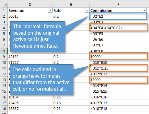
The shortcut to show all of the formulas on a spreadsheet is Ctrl + ~ (tilde). Press it again to toggle back to view the values. You can also press the Show Formulas button on the Formulas tab of the ribbon.

The FORMULATEXT Function

Microsoft introduced the FORMULATEXT function in Excel 2013. The function returns the text of the formula to the cell.

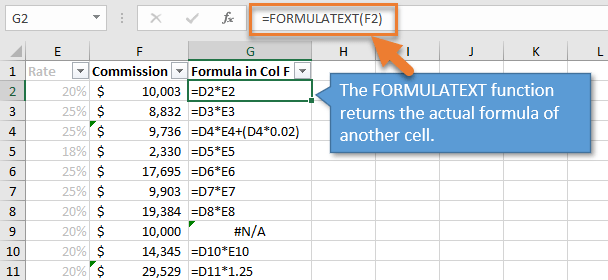
This makes it easy to see both the result of the formulas and the text of the formulas in an adjacent column/row.

You can wrap the function in IFERROR or IFNA to return a different result for cells that do not contain formulas.

=IFNA(FORMULATEXT(F2),"Value")

Using the Go To Special Window

If you’re more of a mouse user, you can also select cells with differences in the Go To Special window.

1. From the Home Tab on the Ribbon, choose the Find & Select button. This brings up a drop-down menu.

2. Click on Go To Special…

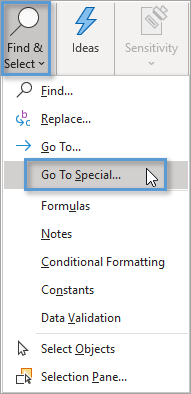
3. This will open up the Go To Special window, where you can select Column differences.

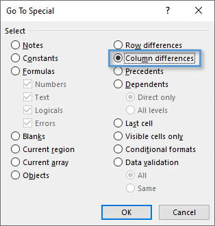
4. When you hit OK, only the cells that have values different from the original active cell will be selected.

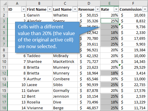
It Works for Rows Too

All of the above instructions work for differences in rows instead of columns. The only change is that the keyboard shortcut is Ctrl + .

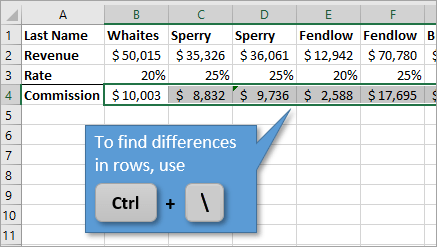
Obviously, when using the Go To Special window, you are going to choose the Row differences option rather than the Column differences.

And as with the columns, you can find differences in values (whether numbers or text), and not just differences in formulas.

Related Post

If you like this keyboard shortcut, check out some of my other favorites in this post: 5 Keyboard Shortcuts for Rows and Columns in Excel.

Conclusion

I hope this tip was helpful, especially if you need to review or audit a spreadsheet for any potential errors in the way it is calculating results. Do you have other tips for auditing workbooks? If so, let us know in the comments below.