
In this example, the goal is to use a formula to check if a specific value exists in a range. The easiest way to do this is to use the COUNTIF function to count occurences of a value in a range, then use the count to create a final result.
COUNTIF function
The COUNTIF function counts cells that meet supplied criteria. The generic syntax looks like this:
=COUNTIF(range,criteria)Range is the range of cells to test, and criteria is a condition that should be tested. COUNTIF returns the number of cells in range that meet the condition defined by criteria. If no cells meet criteria, COUNTIF returns zero. In the example shown, we can use COUNTIF to count the values we are looking for like this
COUNTIF(data,E5)Once the named range data (B5:B16) and cell E5 have been evaluated, we have:
=COUNTIF(data,E5)
=COUNTIF(B5:B16,"Blue")
=1
COUNTIF returns 1 because «Blue» occurs in the range B5:B16 once. Next, we use the greater than operator (>) to run a simple test to force a TRUE or FALSE result:
=COUNTIF(data,B5)>0 // returns TRUE or FALSEBy itself, the formula above will return TRUE or FALSE. The last part of the problem is to return a «Yes» or «No» result. To handle this, we nest the formula above into the IF function like this:
=IF(COUNTIF(data,E5)>0,"Yes","No")This is the formula shown in the worksheet above. As the formula is copied down, COUNTIF returns a count of the value in column E. If the count is greater than zero, the IF function returns «Yes». If the count is zero, IF returns «No».
Slightly abbreviated
It is possible to shorten this formula slightly and get the same result like this:
=IF(COUNTIF(data,E5),"Yes","No")Here, we have remove the «>0» test. Instead, we simply return the count to IF as the logical_test. This works because Excel will treat any non-zero number as TRUE when the number is evaluated as a Boolean.
Testing for a partial match
To test a range to see if it contains a substring (a partial match), you can add a wildcard to the formula. For example, if you have a value to look for in cell C1, and you want to check the range A1:A100 for partial matches, you can configure COUNTIF to look for the value in C1 anywhere in a cell by concatenating asterisks on both sides:
=COUNTIF(A1:A100,"*"&C1&"*")>0
The asterisk (*) is a wildcard for one or more characters. By concatenating asterisks before and after the value in C1, the formula will count the text in C1 anywhere it appears in each cell of the range. To return «Yes» or «No», nest the formula inside the IF function as above.
An alternative formula using MATCH
As an alternative, you can use a formula that uses the MATCH function with the ISNUMBER function instead of COUNTIF:
=ISNUMBER(MATCH(value,range,0))
The MATCH function returns the position of a match (as a number) if found, and #N/A if not found. By wrapping MATCH inside ISNUMBER, the final result will be TRUE when MATCH finds a match and FALSE when MATCH returns #N/A.
EXPLANATION
This tutorial shows how to test if a range does not contain a specific value and return a specified value if the formula tests true or false, by using an Excel formula and VBA.
This tutorial provides one Excel method that can be applied to test if a range does not contain a specific value and return a specified value by using an Excel IF and COUNTIF functions. In this example, if the Excel COUNTIF function returns a value of 0, meaning the range does not have cells with a value of 505, the test is TRUE and the formula will return a «Not in Range» value. Alternatively, if the Excel COUNTIF function returns a value of greater than 0, meaning the range has cells with a value of 505, the test is FALSE and the formula will return a «In Range» value.
This tutorial provides one VBA method that can be applied to test if a range does not contain a specific value and return a specified value and return a specified value.
FORMULA
=IF(COUNTIF(range, value)=0, value_if_true, value_if_false)
ARGUMENTS
range: The range of cells you want to count from.
value: he value that is used to determine which of the cells should be counted, from a specified range, if the cells’ value is equal to this value.
value_if_true: Value to be returned if the range does not contains the specific value.
value_if_false: Value to be returned if the range contains the specific value.
I have two ranges that should be identical (albeit they may be sorted differently). I’m trying to find any values in rangeA that are not in rangeB.
I’m able to find examples that show if values ARE matched in a range, but struggling to find anything if they aren’t.
So far I have:
Sub Compare2()

    Dim test1, cell As Range
    Dim FoundRange As Range

    Set test1 = Sheets("Names").Range("A1:A5")
    For Each cell In test1

        Set FoundRange = Sheets("Queue & Status").Range("A1:A200").Find(what:=test1, LookIn:=xlFormulas, lookat:=xlWhole)

        If FoundRange Is Nothing Then
            MsgBox (cell & " not found")
        End If

    Next cell
End Sub
But it’s showing all values as being not matched, when they are.
![]()
asked Dec 2, 2016 at 2:34
![]()
4
Try this
Sub Compare2()

    Dim test1 As Range
    Dim lookIn As Range
    Dim c As Range
    Dim FoundRange As Range

    Set test1 = Sheets("Names").Range("A1:A5")
    Set lookIn = Sheets("Queue & Status").Range("A1:A200")
    For Each c In test1

        Set FoundRange = lookIn.Find(what:=c.Value, lookIn:=xlFormulas, lookat:=xlWhole)

        If FoundRange Is Nothing Then
            MsgBox (c.Value & " not found")
        End If

    Next c
End Sub
answered Dec 2, 2016 at 3:03
![]()
nightcrawler23nightcrawler23
2,0461 gold badge14 silver badges22 bronze badges
1
what:=test1 should be what:=cell (or even what:=cell.value)
answered Dec 2, 2016 at 2:49
![]()
S MS M
133 silver badges4 bronze badges
Home / Excel Formulas / Check IF a Value Exists in a Range
In Excel, to check if a value exists in a range or not, you can use the COUNTIF function, with the IF function. With COUNTIF you can check for the value and with IF, you can return a result value to show to the user. i.e., Yes or No, Found or Not Found.
In the following example, you have a list of names where you only have first names, and now, you need to check if “Arlene” is there or not.

You can use the following steps:
- First, you need to enter the IF function in cell B1.

- After that, in the first argument (logical test), you need to enter the COUNTIF function there.

- Now, in the COUNTIF function, refer to the range A1:A10.

- Next, in the criteria argument, enter “Glen” and close the parentheses for the COUNTIF Function.

- Additionally, use a greater than sign and enter a zero.

- From here, enter a comma to go to the next argument in the IF, and enter “Yes” in the second argument.

- In the end, enter a comma and enter “No” in the third argument and type the closing parentheses.


The moment you hit enter it returns “Yes”, as you have the value in the range that you have searched for.

=IF(COUNTIF(A1:A10,"Glen")>0,"Yes","No")How this Formula Works
This formula has two parts.

In the first part, we have COUNTIF, which counts the occurrence of the value in the range. And in the second part, you have the IF function that takes the values from the COUNTIF function.
So, if COUNTIF returns any value greater than which means the value is there in the range IF returns Yes. And if COUNTIF returns 0, which means the value is not there in the range and it returns No.
Check for a Value in a Range Partially
There counts to be a situation where you want to check for partial value from a range. In that case, you need to use wildcard characters (asterisk *).
In the following example, we have the same list of names but here is the full name. But we still need to look for the name “Glen”.

=IF(COUNTIF(C1:C10,"*"&"Glen"&"*")>0,"Yes","No")The value you want to search for needs to be enclosed with an asterisk, which we have used in the above example. This tells Excel, to check for the value “Glen” regardless of what is there before and after the value.
Download Sample File
- Ready
And, if you want to Get Smarter than Your Colleagues check out these FREE COURSES to Learn Excel, Excel Skills, and Excel Tips and Tricks.
We often compare one range values with another range to check for duplicates. But how to check if one range values exist in another range in Excel? We will learn in this article how to check if a range contains a value not in another range in Excel.
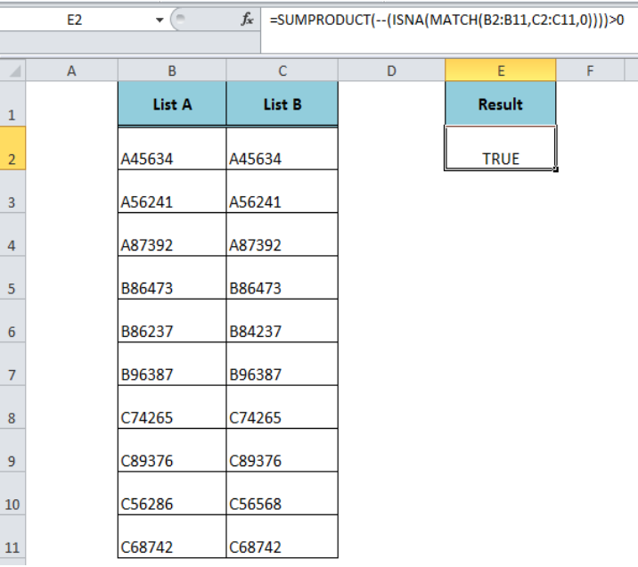 Figure 1. Check If a Range Contains a Value Not in Another Range
Formula Syntax
The generic formula syntax is;
=SUMPRODUCT(--(ISNA(MATCH(range1,range2,0))))>0
In this formula, we use the SUMPRODUCT function along with MATCH and ISNA function. This formula checks if range one contains at least one or more values that are not part of another range and returns TRUE, else it returns FALSE.
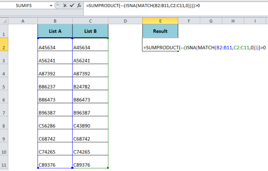 Figure 2. Formula Syntax
Suppose we have two lists of students’ roll numbers and we want to check if List A contains any values (one or more values) that are not in List B. Hence, the formula compares List A (range B2: B11) with List B (range C2: C11) and returns TRUE if List A contains at least one or more values not in List B, such as;
=SUMPRODUCT(--(ISNA(MATCH(B2:B11,C2:C11,0))))>0
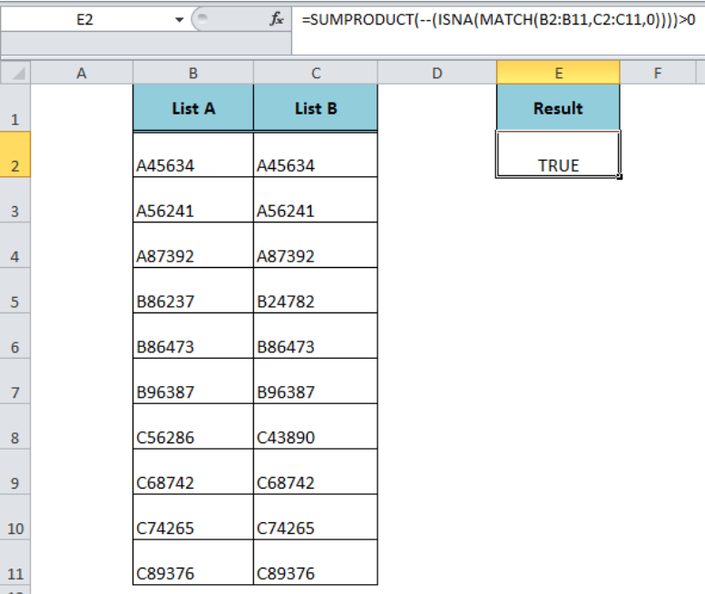 Figure 3. The Formula Result
How Formula Works
The MATCH function returns the relative positions of range B2: B11 values that exactly match in range C2: C11, and returns the #NA error value(s) where range B2: B11 values are not found in range C2: C11 as an array. Select the MATCH part of the formula in the formula bar and press F9 to view the resulting array.
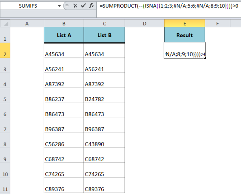 Figure 4. Resulting Array of the MATCH Function
The ISNA function checks for the #NA error values and returns TRUE, else returns FALSE. Hence, it converts the array returned by the MATCH function into an array of TRUE and FALSE logical values, such as;
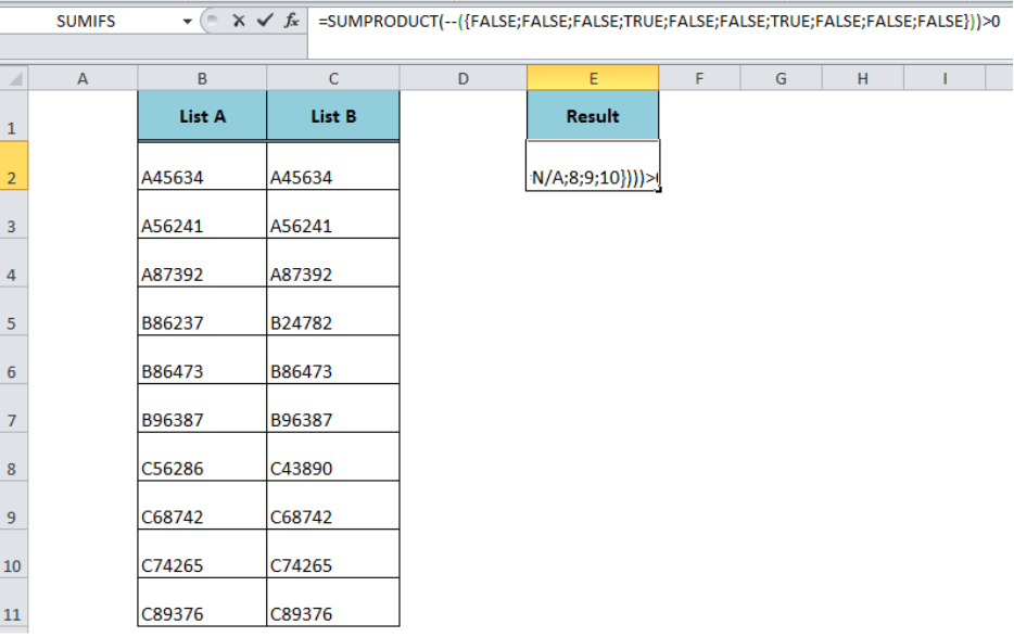 Figure 5. The array of Logical Values Return by the ISNA Function
The double dash (–) symbol converts the TRUE and FALSE logical values into an array of 1s and 0s. The SUMPRODUCT function sums this final array of 1s and 0s and compares the result with 0 and returns TRUE if the sum of values is greater than 0.
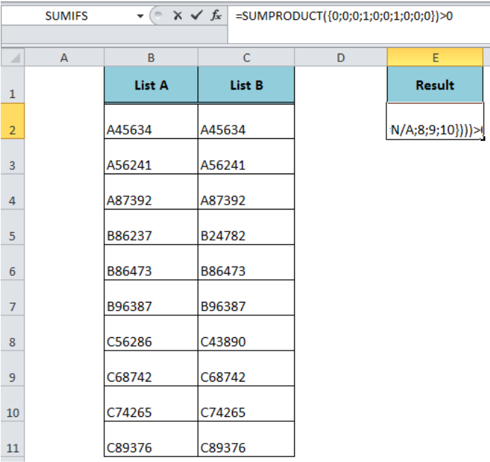 Figure 6. Final Array of 1s and 0s
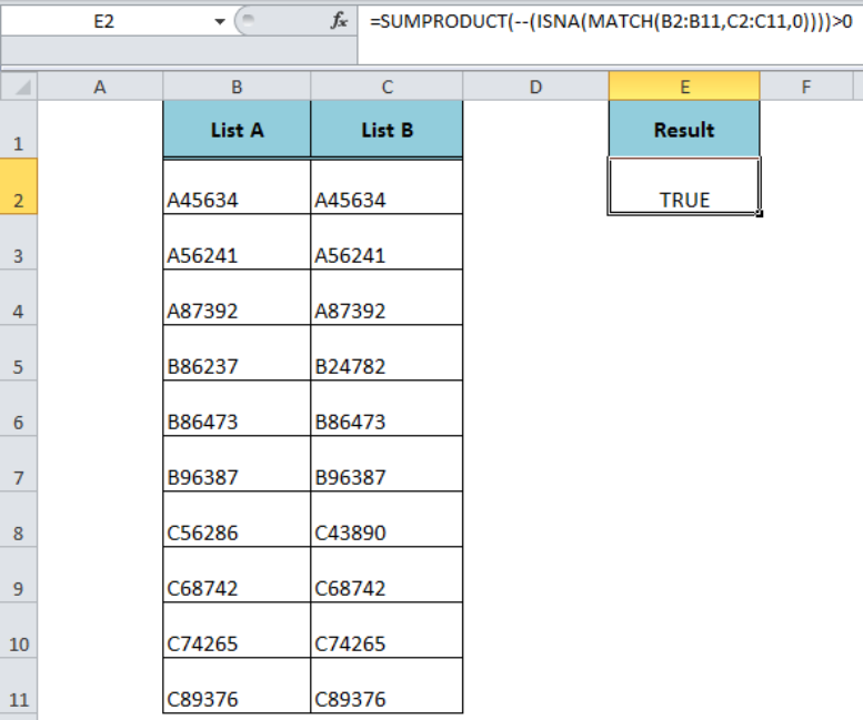 Figure 7. Final Result of the Formula
Instant Connection to an Expert through our Excelchat Service:
Most of the time, the problem you will need to solve will be more complex than a simple application of a formula or function. If you want to save hours of research and frustration, try our live Excelchat service! Our Excel Experts are available 24/7 to answer any Excel question you may have. We guarantee a connection within 30 seconds and a customized solution within 20 minutes.