Excel if cell not error - Word и Excel - помощь в работе с программами

Excel for Microsoft 365 Excel for Microsoft 365 for Mac Excel for the web Excel 2021 Excel 2021 for Mac Excel 2019 Excel 2019 for Mac Excel 2016 Excel 2016 for Mac Excel 2013 Excel Web App Excel 2010 Excel 2007 Excel for Mac 2011 Excel Starter 2010 More…Less

You can use the IFERROR function to trap and handle errors in a formula. IFERROR returns a value you specify if a formula evaluates to an error; otherwise, it returns the result of the formula.

Syntax

IFERROR(value, value_if_error)

The IFERROR function syntax has the following arguments:

value Required. The argument that is checked for an error.
value_if_error Required. The value to return if the formula evaluates to an error. The following error types are evaluated: #N/A, #VALUE!, #REF!, #DIV/0!, #NUM!, #NAME?, or #NULL!.

Remarks

If value or value_if_error is an empty cell, IFERROR treats it as an empty string value («»).
If value is an array formula, IFERROR returns an array of results for each cell in the range specified in value. See the second example below.

Examples

Copy the example data in the following table, and paste it in cell A1 of a new Excel worksheet. For formulas to show results, select them, press F2, and then press Enter.

Quota	Units Sold
210	35
55	0
	23
Formula	Description	Result
=IFERROR(A2/B2, «Error in calculation»)	Checks for an error in the formula in the first argument (divide 210 by 35), finds no error, and then returns the results of the formula	6
=IFERROR(A3/B3, «Error in calculation»)	Checks for an error in the formula in the first argument (divide 55 by 0), finds a division by 0 error, and then returns value_if_error	Error in calculation
=IFERROR(A4/B4, «Error in calculation»)	Checks for an error in the formula in the first argument (divide «» by 23), finds no error, and then returns the results of the formula.	0

Example 2

Quota	Units Sold	Ratio
210	35	6
55	0	Error in calculation
	23	0
Formula	Description	Result
=C2	Checks for an error in the formula in the first argument in the first element of the array (A2/B2 or divide 210 by 35), finds no error, and then returns the result of the formula	6
=C3	Checks for an error in the formula in the first argument in the second element of the array (A3/B3 or divide 55 by 0), finds a division by 0 error, and then returns value_if_error	Error in calculation
=C4	Checks for an error in the formula in the first argument in the third element of the array (A4/B4 or divide «» by 23), finds no error, and then returns the result of the formula	0

	Note: If you have a current version of Microsoft 365, then you can input the formula in the top-left-cell of the output range, then press ENTER to confirm the formula as a dynamic array formula. Otherwise, the formula must be entered as a legacy array formula by first selecting the output range, input the formula in the top-left-cell of the output range, then press CTRL+SHIFT+ENTER to confirm it. Excel inserts curly brackets at the beginning and end of the formula for you. For more information on array formulas, see Guidelines and examples of array formulas.

Need more help?

You can always ask an expert in the Excel Tech Community or get support in the Answers community.

Need more help?

Источник

Date yes Add (Subtract) Days to a Date Concatenate Dates Convert Date to Number Convert Date to Text Month Name to Number Create Date Range from Dates Day Number of Year Month Name from Date First Day of Month Add (Subtract) Weeks to a Date If Functions with Dates Max Date Number of Days Between Dates Number of Days in a Month Number of Weeks Between Dates Number of Years Between Dates Split Date & Time into Separate Cells Countdown Remaining Days Insert Dates Random Date Generator Using Dynamic Ranges — Year to Date Values Add (Subtract) Years to a Date Date Formula Examples Extract Day from Date Get Day Name from Date Count Days Left in Month / Year Count Workdays Left in Month / Year Get Last Day of Month Last Business Day of Month / Year Number of Work / Business Days in Month Weekday Abbreviations Auto Populate Dates Number of Months Between Dates Quarter from a Date Years of Service Change Date Format Compare Dates Time yes Add (Subtract) Hours to Time Add (Subtract) Minutes to Time Add (Subtract) Seconds to Time Add Up time (Total Time) Time Differences Change Time Format Convert Minutes to Hours Convert Time to Decimal Convert Time to Hours Convert Time to Minutes Convert Time to Seconds Military Time Round Time to Nearest 15 Minutes Overtime Calculator Number of Hours Between Times Convert Seconds to Minutes, Hours, or Time Count Hours Worked Time Differences Time Format — Show Minutes Seconds Text yes Add Commas to Cells Get First Word from Text Capitalize First Letter Clean & Format Phone #s Remove Extra Trailing / Leading Spaces Add Spaces to Cell Assign Number Value to Text Combine Cells with Comma Combine First and Last Names Convert Text String to Date Convert Text to Number Extract Text From Cell Get Last Word Remove Unwated Characters Extract Text Before or After Character How to Split Text String by Space, Comma, & More Remove Special Characters Remove First Characters from Left Substitute Multiple Values Switch First & Last Names w/ Commas Remove Specific Text from a Cell Extract Text Between Characters (Ex. Parenthesis) Add Leading Zeros to a Number Remove Line Breaks from Text Remove all Numbers from Text Reverse Text Remove Non-Numeric Characters Remove Last Character(s) From Right Separate First and Last Names Separate Text & Numbers Round yes Round Formulas Round Price to Nearest Dollar or Cent Round to Nearest 10, 100, or 1000 Round to Nearest 5 or .5 Round Percentages Round to Significant Figures Count yes Count Blank and Non-blank Cells Count Cells Between Two Numbers Count Cells not Equal to Count if Cells are in Range Count Times Word Appears in Cell Count Words in Cell Count Specific Characters in Column Count Total Number of Characters in Column Count Cells that Equal one of two Results Count Cells that do not Contain Count Cells that Contain Specific Text Count Unique Values in Range Countif — Multiple Criteria Count Total Number of Cells in Range Count Cells with Any Text Count Total Cells in a Table Lookup yes Two Dimensional VLOOKUP VLOOKUP Simple Example Vlookup — Multiple Matches Case Sensitive Lookup Case Sensitive VLOOKUP Sum if — VLOOKUP Case Sensitive Lookup Case Sensitive VLOOKUP Find Duplicates w/ VLOOKUP or MATCH INDEX MATCH MATCH Lookup — Return Cell Address (Not Value) Lookup Last Value in Column or Row Reverse VLOOKUP (Right to Left) Risk Score Bucket with VLOOKUP Sum with a VLOOKUP Function VLOOKUP & INDIRECT VLOOKUP Concatenate VLOOKUP Contains (Partial Match) 17 Reasons Why Your XLOOKUP is Not Working Double (Nested) XLOOKUP — Dynamic Columns IFERROR (& IFNA) XLOOKUP Lookup Min / Max Value Nested VLOOKUP Top 11 Alternatives to VLOOKUP (Updated 2022!) VLOOKUP – Dynamic Column Reference VLOOKUP – Fix #N/A Error VLOOKUP – Multiple Sheets at Once VLOOKUP & HLOOKUP Combined VLOOKUP & MATCH Combined VLOOKUP Between Worksheets or Spreadsheets VLOOKUP Duplicate Values VLOOKUP Letter Grades VLOOKUP Return Multiple Columns VLOOKUP Returns 0? Return Blank Instead VLOOKUP w/o #N/A Error XLOOKUP Multiple Sheets at Once XLOOKUP Between Worksheets or Spreadsheets XLOOKUP by Date XLOOKUP Duplicate Values XLOOKUP Multiple Criteria XLOOKUP Return Multiple Columns XLOOKUP Returns 0? Return Blank Instead XLOOKUP Text XLOOKUP with IF XLOOKUP With If Statement Misc. yes Sort Multiple Columns Use Cell Value in Formula Percentage Change Between Numbers Percentage Breakdown Rank Values Add Spaces to Cell CAGR Formula Average Time Decimal Part of Number Integer Part of a Number Compare Items in a List Dealing with NA() Errors Get Worksheet Name Wildcard Characters Hyperlink to Current Folder Compound Interest Formula Percentage Increase Create Random Groups Sort with the Small and Large Functions Non-volatile Function Alternatives Decrease a Number by a Percentage Calculate Percent Variance Profit Margin Calculator Convert Column Number to Letter Get Full Address of Named Range Insert File Name Insert Path Latitute / Longitude Functions Replace Negative Values Reverse List Range Convert State Name to Abbreviation Create Dynamic Hyperlinks Custom Sort List with Formula Data Validation — Custom Formulas Dynamic Sheet Reference (INDIRECT) Reference Cell in Another Sheet or Workbook Get Cell Value by Address Get Worksheet Name Increment Cell Reference List Sheet Names List Skipped Numbers in Sequence Return Address of Max Value in Range Search by Keywords Select Every Other (or Every nth) Row Basics yes Cell Reference Basics — A1, R1C1, 3d, etc. Add Up (Sum) Entire Column or Row Into to Dynamic Array Formulas Conversions yes Convert Time Zones Convert Celsius to Fahrenheit Convert Pounds to Kilograms Convert Time to Unix Time Convert Feet to Meters Convert Centimeters to Inches Convert Kilometers to Miles Convert Inches to Feet Convert Date to Julian Format Convert Column Letter to Number Tests yes Test if a Range Contains any Text Test if any Cell in Range is Number Test if a Cell Contains a Specific Value Test if Cell Contains Any Number Test if Cell Contains Specific Number Test if Cell is Number or Text If yes Percentile If Subtotal If Sumproduct If Large If and Small If Median If Concatentate If Max If Rank If TEXTJOIN If Sum yes Sum if — Begins With / Ends With Sum if — Month or Year to Date Sum if — By Year Sum if — Blank / Non-Blank Sum if — Horizontal Sum Count / Sum If — Cell Color INDIRECT Sum Sum If — Across Multiple Sheets Sum If — By Month Sum If — Cells Not Equal To Sum If — Not Blank Sum if — Between Values Sum If — Week Number Sum Text Sum if — By Category or Group Sum if — Cell Contains Specific Text (Wildcards) Sum if — Date Rnage Sum if — Dates Equal Sum if — Day of Week Sum if — Greater Than Sum if — Less Than Average yes Average Non-Zero Values Average If — Not Blank Average — Ignore 0 Average — Ignore Errors Math yes Multiplication Table Cube Roots nth Roots Square Numbers Square Roots Calculations yes Calculate a Ratio Calculate Age KILLLLLLL Calculate Loan Payments GPA Formula Calculate VAT Tax How to Grade Formulas Find yes Find a Number in a Column / Workbook Find Most Frequent Numbers Find Smallest n Values Find nth Occurance of Character in Text Find and Extract Number from String Find Earliest or Latest Date Based on Criteria Find First Cell with Any Value Find Last Row Find Last Row with Data Find Missing Values Find Largest n Values Most Frequent Number Conditional Formatting yes Conditional Format — Dates & Times Conditional Format — Highlight Blank Cells New Functions XLOOKUP Replaces VLOOKUP, HLOOKUP, and INDEX / MATCH Logical yes AND Checks whether all conditions are met. TRUE/FALSE IF If condition is met, do something, if not, do something else. IFERROR If result is an error then do something else. NOT Changes TRUE to FALSE and FALSE to TRUE. OR Checks whether any conditions are met. TRUE/FALSE XOR Checks whether one and only one condition is met. TRUE/FALSE Lookup & Reference yes FALSE The logical value: FALSE. TRUE The logical value: TRUE. ADDRESS Returns a cell address as text. AREAS Returns the number of areas in a reference. CHOOSE Chooses a value from a list based on it’s position number. COLUMN Returns the column number of a cell reference. COLUMNS Returns the number of columns in an array. HLOOKUP Lookup a value in the first row and return a value. HYPERLINK Creates a clickable link. INDEX Returns a value based on it’s column and row numbers. INDIRECT Creates a cell reference from text. LOOKUP Looks up values either horizontally or vertically. MATCH Searches for a value in a list and returns its position. OFFSET Creates a reference offset from a starting point. ROW Returns the row number of a cell reference. ROWS Returns the number of rows in an array. TRANSPOSE Flips the oriention of a range of cells. VLOOKUP Lookup a value in the first column and return a value. Date & Time yes DATE Returns a date from year, month, and day. DATEDIF Number of days, months or years between two dates. DATEVALUE Converts a date stored as text into a valid date DAY Returns the day as a number (1-31). DAYS Returns the number of days between two dates. DAYS360 Returns days between 2 dates in a 360 day year. EDATE Returns a date, n months away from a start date. EOMONTH Returns the last day of the month, n months away date. HOUR Returns the hour as a number (0-23). MINUTE Returns the minute as a number (0-59). MONTH Returns the month as a number (1-12). NETWORKDAYS Number of working days between 2 dates. NETWORKDAYS.INTL Working days between 2 dates, custom weekends. NOW Returns the current date and time. SECOND Returns the second as a number (0-59) TIME Returns the time from a hour, minute, and second. TIMEVALUE Converts a time stored as text into a valid time. TODAY Returns the current date. WEEKDAY Returns the day of the week as a number (1-7). WEEKNUM Returns the week number in a year (1-52). WORKDAY The date n working days from a date. WORKDAY.INTL The date n working days from a date, custom weekends. YEAR Returns the year. YEARFRAC Returns the fraction of a year between 2 dates. Engineering yes CONVERT Convert number from one unit to another. Financial yes FV Calculates the future value. PV Calculates the present value. NPER Calculates the total number of payment periods. PMT Calculates the payment amount. RATE Calculates the interest Rate. NPV Calculates the net present value. IRR The internal rate of return for a set of periodic CFs. XIRR The internal rate of return for a set of non-periodic CFs. PRICE Calculates the price of a bond. YIELD Calculates the bond yield. INTRATE The interest rate of a fully invested security. Information yes CELL Returns information about a cell. ERROR.TYPE Returns a value representing the cell error. ISBLANK Test if cell is blank. TRUE/FALSE ISERR Test if cell value is an error, ignores #N/A. TRUE/FALSE ISERROR Test if cell value is an error. TRUE/FALSE ISEVEN Test if cell value is even. TRUE/FALSE ISFORMULA Test if cell is a formula. TRUE/FALSE ISLOGICAL Test if cell is logical (TRUE or FALSE). TRUE/FALSE ISNA Test if cell value is #N/A. TRUE/FALSE ISNONTEXT Test if cell is not text (blank cells are not text). TRUE/FALSE ISNUMBER Test if cell is a number. TRUE/FALSE ISODD Test if cell value is odd. TRUE/FALSE ISREF Test if cell value is a reference. TRUE/FALSE ISTEXT Test if cell is text. TRUE/FALSE N Converts a value to a number. NA Returns the error: #N/A. TYPE Returns the type of value in a cell. Math yes ABS Calculates the absolute value of a number. AGGREGATE Define and perform calculations for a database or a list. CEILING Rounds a number up, to the nearest specified multiple. COS Returns the cosine of an angle. DEGREES Converts radians to degrees. DSUM Sums database records that meet certain criteria. EVEN Rounds to the nearest even integer. EXP Calculates the exponential value for a given number. FACT Returns the factorial. FLOOR Rounds a number down, to the nearest specified multiple. GCD Returns the greatest common divisor. INT Rounds a number down to the nearest integer. LCM Returns the least common multiple. LN Returns the natural logarithm of a number. LOG Returns the logarithm of a number to a specified base. LOG10 Returns the base-10 logarithm of a number. MOD Returns the remainder after dividing. MROUND Rounds a number to a specified multiple. ODD Rounds to the nearest odd integer. PI The value of PI. POWER Calculates a number raised to a power. PRODUCT Multiplies an array of numbers. QUOTIENT Returns the integer result of division. RADIANS Converts an angle into radians. RAND Calculates a random number between 0 and 1. RANDBETWEEN Calculates a random number between two numbers. ROUND Rounds a number to a specified number of digits. ROUNDDOWN Rounds a number down (towards zero). ROUNDUP Rounds a number up (away from zero). SIGN Returns the sign of a number. SIN Returns the sine of an angle. SQRT Calculates the square root of a number. SUBTOTAL Returns a summary statistic for a series of data. SUM Adds numbers together. SUMIF Sums numbers that meet a criteria. SUMIFS Sums numbers that meet multiple criteria. SUMPRODUCT Multiplies arrays of numbers and sums the resultant array. TAN Returns the tangent of an angle. TRUNC Truncates a number to a specific number of digits. Stats yes AVERAGE Averages numbers. AVERAGEA Averages numbers. Includes text & FALSE =0, TRUE =1. AVERAGEIF Averages numbers that meet a criteria. AVERAGEIFS Averages numbers that meet multiple criteria. CORREL Calculates the correlation of two series. COUNT Counts cells that contain a number. COUNTA Count cells that are non-blank. COUNTBLANK Counts cells that are blank. COUNTIF Counts cells that meet a criteria. COUNTIFS Counts cells that meet multiple criteria. FORECAST Predict future y-values from linear trend line. FREQUENCY Counts values that fall within specified ranges. GROWTH Calculates Y values based on exponential growth. INTERCEPT Calculates the Y intercept for a best-fit line. LARGE Returns the kth largest value. LINEST Returns statistics about a trendline. MAX Returns the largest number. MEDIAN Returns the median number. MIN Returns the smallest number. MODE Returns the most common number. PERCENTILE Returns the kth percentile. PERCENTILE.INC Returns the kth percentile. Where k is inclusive. PERCENTILE.EXC Returns the kth percentile. Where k is exclusive. QUARTILE Returns the specified quartile value. QUARTILE.INC Returns the specified quartile value. Inclusive. QUARTILE.EXC Returns the specified quartile value. Exclusive. RANK Rank of a number within a series. RANK.AVG Rank of a number within a series. Averages. RANK.EQ Rank of a number within a series. Top Rank. SLOPE Calculates the slope from linear regression. SMALL Returns the kth smallest value. STDEV Calculates the standard deviation. STDEV.P Calculates the SD of an entire population. STDEV.S Calculates the SD of a sample. STDEVP Calculates the SD of an entire population TREND Calculates Y values based on a trendline. Text yes CHAR Returns a character specified by a code. CLEAN Removes all non-printable characters. CODE Returns the numeric code for a character. CONCATENATE Combines text together. DOLLAR Converts a number to text in currency format. EXACT Test if cells are exactly equal. Case-sensitive. TRUE/FALSE FIND Locates position of text within a cell.Case-sensitive. LEFT Truncates text a number of characters from the left. LEN Counts number of characters in text. LOWER Converts text to lower case. MID Extracts text from the middle of a cell. PROPER Converts text to proper case. REPLACE Replaces text based on it’s location. REPT Repeats text a number of times. RIGHT Truncates text a number of characters from the right. SEARCH Locates position of text within a cell.Not Case-sensitive. SUBSTITUTE Finds and replaces text. Case-sensitive. TEXT Converts a value into text with a specific number format. TRIM Removes all extra spaces from text. UPPER Converts text to upper case. VALUE Converts a number stored as text into a number.

Источник

ISERROR is a logical function that is used to identify whether the cells being referred to have an error or not. This function identifies all the mistakes. If any error is found in the cell, it returns “TRUE” as a result, and if the cell has no errors, it gives “FALSE” as a result. This function takes a cell reference as an argument.

ISERROR function in Excel checks if any given expression returns an error in Excel.

For example, suppose you have a dataset and applied the ISERROR formula to divide the number by 0. In such a scenario, the ISERROR Excel function verifies the value and returns ” TRUE” if it possesses an error. Therefore, Excel displays the #DIV/0! Error. Conversely, as a result, it provides ” FALSE” if it does not consist of any error.

ISERROR Function in Excel
- ISERROR Formula in Excel
  - Arguments used for ISERROR Function.
  - Returns
- ISERROR in Excel – Illustration
- How to Use the ISERROR Function in Excel?
- ISERROR in Excel Example #1
- ISERROR in Excel Example #2
- ISERROR in Excel Example #3
- Things to Know about the ISERROR Function in Excel
- ISERROR Excel Function Video
- Recommended Articles

ISERROR Formula in Excel

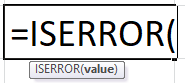
Arguments used for ISERROR Function.

Value: The expression or value to be tested for error.

The value can be a number, text, mathematical operation, or expression.

Returns

The output of ISERROR in Excel is a logical expression. If the supplied argument gives an error in Excel, it returns “TRUE.” Otherwise, it returns “FALSE.” For error messages- #N/A, #VALUE!, #REF!, #DIV/0!, #NUM!, #NAME?, and #NULL! generated by Excel, the function returns “TRUE.”

ISERROR in Excel – Illustration

Suppose we want to see if a number gives an error when divided by another number.

We know that a number, when divided by zero, gives an error in ExcelErrors in excel are common and often occur at times of applying formulas. The list of nine most common excel errors are — #DIV/0, #N/A, #NAME?, #NULL!, #NUM!, #REF!, #VALUE!, #####, Circular Reference.read more. Let us check if 21/0 provides an error using the ISERROR in Excel. To do this, we must type the syntax:

= ISERROR ( 21/0 )

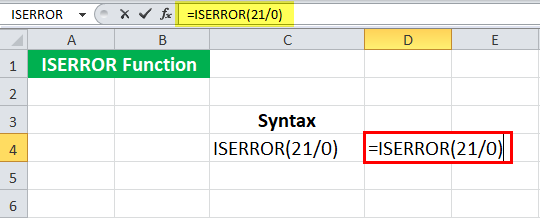
Press the “Enter” key.

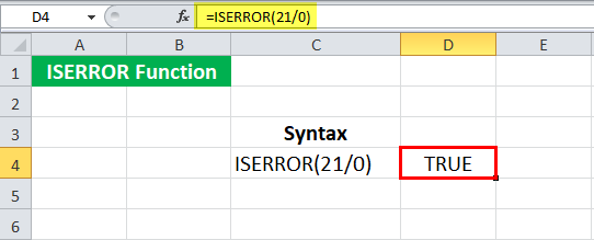
It returns “TRUE.”

We can also refer to cell references in the ISERROR in Excel. Let us now check what will happen when we divide one cell by an empty cell.

When we enter the syntax:
= ISERROR ( A5/B5 )
Given that B5 is an empty cell.

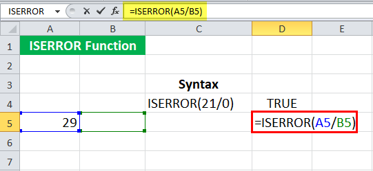
The ISERROR in Excel will return “TRUE.”

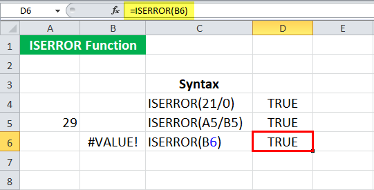
We can also check if any cell contains an error message. Suppose cell B6 has #VALUE! Which is an error in Excel. We may directly input the cell reference in the ISERROR in Excel to check if there is an error message or not as:

= ISERROR ( B6 )

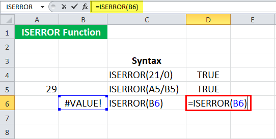
The ISERROR function in Excel will return “TRUE.”

Suppose we refer to an empty cell (B7 in this case) and use the following syntax:

= ISERROR (B7)

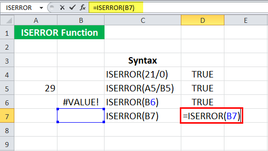
Press the “Enter” key.

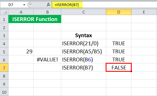
The ISERROR function in Excel may return “FALSE” since the Excel ISERROR function does not check for an empty cell. A blank cell is often considered zero in Excel. So, as we may have noticed above, if we refer to an empty cell in an operation such as division, it will be an error as it is trying to divide it by zero and thus returns “TRUE.”

How to Use the ISERROR Function in Excel?

The ISERROR function in Excel is used to identify cells containing an error. For example, there is often an occurrence of missing values in the data. If a further operation is carried out on such cells, the Excel may get an error. Similarly, if we divide any number by zero, it returns an error. Such errors further intervene if any other operation is carried out on these cells. In such cases, we can first check if there is an error in the operation. If yes, we can choose not to include such cells or modify the operation later.

You can download this ISERROR Function Excel Template here – ISERROR Function Excel Template

ISERROR in Excel Example #1

Suppose we have the actual and forecast values of an experiment. The values are given in cells B4: C15.

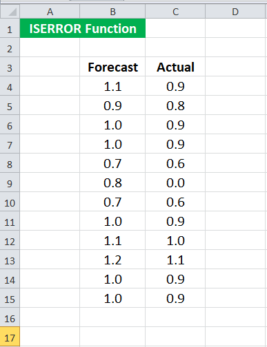
We want to calculate the error rate in this experiment, which is given as (Actual – Forecast) / Actual. However, we also know that some of the actual values are zero, and the error rate for such actual values will give an error. Therefore, we have decided to calculate the error for only those experiments which do not provide an error. To do this, we may use the following syntax for the first set of values:

We apply the ISERROR formula in Excel = IF( ISERROR ( (C4-B4) / C4 ), “” , (C4-B4) / C4)

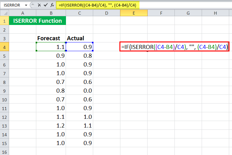
Since the first experimental values do not have any error in calculating the error rate, it will return the error rate.

We will get -0.129

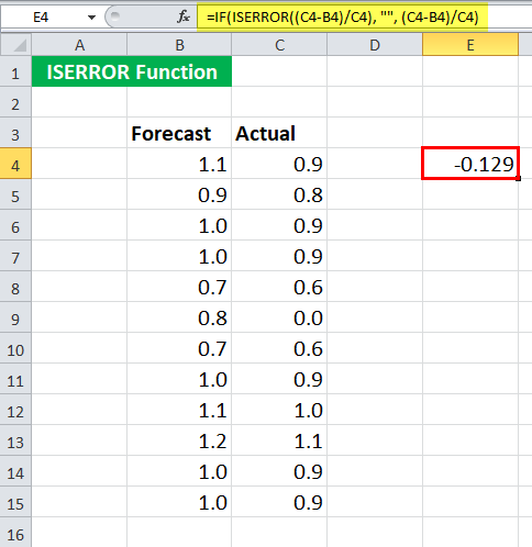
You may now drag it to the rest of the cells.

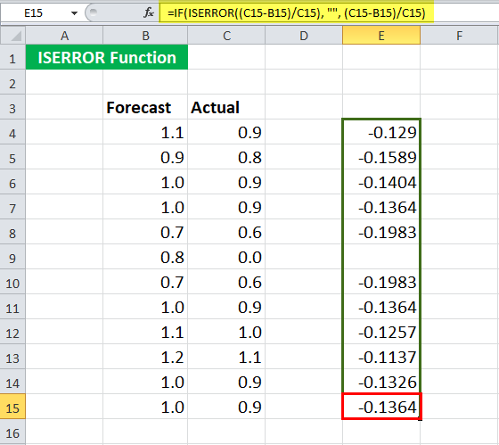
We will realize that the syntax returns no value when the actual value is zero (cell C9).

Now, let us see the syntax in detail.

= IF( ISERROR ( (C4-B4) / C4 ), “” , (C4-B4) / C4 )

ISERROR ( (C4-B4) / C4 ) will check if the mathematical operation (C4-B4) / C4 gives an error. In this case, it will return “FALSE.”
If (ISERROR ( (C4-B4) / C4 ) ) returns “TRUE,” the IF function will not return anything.
If (ISERROR ( (C4-B4) / C4 ) ) returns “FALSE,” the IF function will return (C4-B4) / C4.

ISERROR in Excel Example #2

Suppose we are given some data in B4:B10. Some of the cells contain errors.

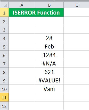
We want to check how many cells right from B4: B10 have an error. To do this, we may use the following ISERROR formula in Excel:

= SUMPRODUCT ( — ISERROR ( B4:B10 ) )

And press the “Enter” key.

ISERROR in Excel will return 2 as there are two errors, i.e., #N/A and #VALUE!#VALUE! Error in Excel represents that the reference cell the user has either entered an incorrect formula or used a wrong data type (mostly numerical data). Sometimes, it is difficult to identify the kind of mistake behind this error.read more.

Let us see the syntax in detail:

ISERROR ( B4:B10 ) will look for errors in B4:B10 and return an array of TRUE or FALSE. Here, it will return {FALSE; FALSE; FALSE; TRUE; FALSE; TRUE; FALSE}
— ISERROR ( B4:B10 ) will then coerce TRUE/ FALSE to 0 and 1. It will return {0; 0; 0; 1; 0; 1; 0}
SUMPRODUCT (– ISERROR ( B4:B10 ) ) will then sum {0; 0; 0; 1; 0; 1; 0} and return 2.

ISERROR in Excel Example #3

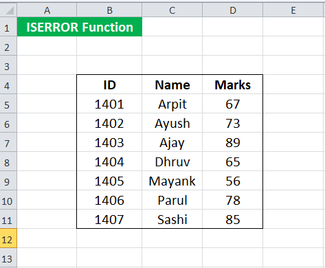
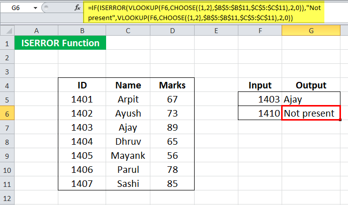
Suppose we have the enrollment ID, name, and marks of students enrolled in the course, given in cells B5:D11.

We must search for the student name given its enrollment ID several times. Now, we want to make the search easier by writing a syntax such that:

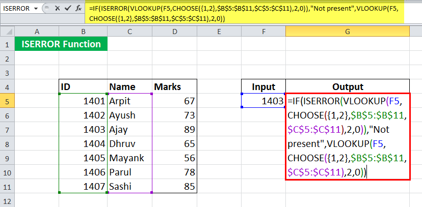
For any given ID, it should be able to give the corresponding name. Sometimes, the enrollment ID may not be present on the list. In such cases, it should return “Not found.” We can do this by using the ISERROR formula in Excel:

= IF( ISERROR( VLOOKUP( F5, CHOOSE( {1,2}, $B$5:$B$11, $C$5:$C$11 ) , 2, 0) ), “Not present”, VLOOKUP( F5, CHOOSE( {1,2}, $B$5:$B$11, $C$5:$C$11 ), 2, 0) )

Let us look at the ISERROR formula in Excel first:

CHOOSE( {1,2}, $B$5:$B$11, $C$5:$C$11 ) will make an array and return {1401,”Arpit”; 1402, “Ayush”; 1403, “Ajay”; 1404, “Dhruv”; 1405, “Mayank”; 1406, “Parul”; 1407, “Sashi”}
VLOOKUP( F5, CHOOSE( {1,2}, $B$5:$B$11, $C$5:$C$11 ) , 2, 0) ) will then look for F5 in the array and return its 2^nd
ISERROR( VLOOKUP( F5, CHOOSE(..) ) will check if there is an error in the function and return TRUE or FALSE.
IF (ISERROR( VLOOKUP( F5, CHOOSE(..) ), “Not present,” VLOOKUP( F5, CHOOSE() )) will return the corresponding name of the student if present. Else it will return “Not present.”

Use the ISERROR formula in Excel For 1403 in cell F5.

It will return the name “Ajay.”

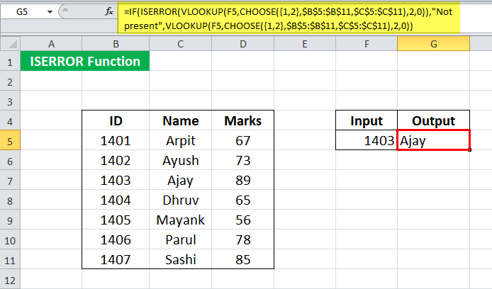
For 1410, the syntax will return “Not present.”

Things to Know about the ISERROR Function in Excel

The ISERROR function in Excel checks if any given expression returns an error.
It returns logical values, “TRUE” or “FALSE.”
It tests for #N/A, #VALUE!, #REF!, #DIV/0!, #NUM!, #NAME?, and #NULL!.

ISERROR Excel Function Video

Return value

The value you specify for error conditions.

Usage notes

The IFERROR function is used to catch errors and return a more friendly result or message when an error is detected. When a formula returns a normal result, the IFERROR function returns that result. When a formula returns an error, IFERROR returns an alternative result. IFERROR is an elegant way to trap and manage errors. The IFERROR function is a modern alternative to the ISERROR function.

Use the IFERROR function to trap and handle errors produced by other formulas or functions. IFERROR checks for the following errors: #N/A, #VALUE!, #REF!, #DIV/0!, #NUM!, #NAME?, or #NULL!.

Example #1

In the example shown, the formula in E5 copied down is:

=IFERROR(C5/D5,0)

This formula catches the #DIV/0! error that occurs when Qty is empty or zero, and replaces it with zero.

Example #2

For example, if A1 contains 10, B1 is blank, and C1 contains the formula =A1/B1, the following formula will catch the #DIV/0! error that results from dividing A1 by B1:

=IFERROR (A1/B1,"Please enter a value in B1")

As long as B1 is empty, C1 will display the message «Please enter a value in B1» if B1 is blank or zero. When a number is entered in B1, the formula will return the result of A1/B1.

Example #3

You can also use the IFERROR function to catch the #N/A error thrown by VLOOKUP when a lookup value isn’t found. The syntax looks like this:

=IFERROR(VLOOKUP(value,data,column,0),"Not found")

In this example, when VLOOKUP returns a result, IFERROR functions that result. If VLOOKUP returns #N/A error because a lookup value isn’t found, IFERROR returns «Not Found».

IFERROR or IFNA?

The IFERROR function is a useful function, but it is a blunt instrument since it will trap many kinds of errors. For example, if there’s a typo in a formula, Excel may return the #NAME? error, but IFERROR will suppress the error and return the alternative result. This can obscure an important problem. In many cases, it makes more sense to use the IFNA function, which only traps the #N/A error.

Other error functions

Excel provides a number of error-related functions, each with a different behavior:

The ISERR function returns TRUE for any error type except the #N/A error.
The ISERROR function returns TRUE for any error.
The ISNA function returns TRUE for #N/A errors only.
The ERROR.TYPE function returns the numeric code for a given error.
The IFERROR function traps errors and provides an alternative result.
The IFNA function traps #N/A errors and provides an alternative result.

Notes

If value is empty, it is evaluated as an empty string («») and not an error.
If value_if_error is supplied as an empty string («»), no message is displayed when an error is detected.
In Excel 2013+, you can use the IFNA function to trap and handle #N/A errors specifically.

Источник

Содержание

IFERROR function
Syntax
Remarks
Examples
Example 2
Need more help?
How to correct a #VALUE! error in the IF function
Problem: The argument refers to error values
Problem: The syntax is incorrect
Need more help?
ISERROR Excel Function
ISERROR Function in Excel
ISERROR Formula in Excel
Returns
ISERROR in Excel – Illustration
How to Use the ISERROR Function in Excel?
ISERROR in Excel Example #1
ISERROR in Excel Example #2
ISERROR in Excel Example #3
Things to Know about the ISERROR Function in Excel
ISERROR Excel Function Video
Recommended Articles

IFERROR function

You can use the IFERROR function to trap and handle errors in a formula. IFERROR returns a value you specify if a formula evaluates to an error; otherwise, it returns the result of the formula.

Syntax

The IFERROR function syntax has the following arguments:

value Required. The argument that is checked for an error.

value_if_error Required. The value to return if the formula evaluates to an error. The following error types are evaluated: #N/A, #VALUE!, #REF!, #DIV/0!, #NUM!, #NAME?, or #NULL!.

If value or value_if_error is an empty cell, IFERROR treats it as an empty string value («»).

If value is an array formula, IFERROR returns an array of results for each cell in the range specified in value. See the second example below.

Examples

Copy the example data in the following table, and paste it in cell A1 of a new Excel worksheet. For formulas to show results, select them, press F2, and then press Enter.

=IFERROR(A2/B2, «Error in calculation»)

Checks for an error in the formula in the first argument (divide 210 by 35), finds no error, and then returns the results of the formula

=IFERROR(A3/B3, «Error in calculation»)

Checks for an error in the formula in the first argument (divide 55 by 0), finds a division by 0 error, and then returns value_if_error

Error in calculation

=IFERROR(A4/B4, «Error in calculation»)

Checks for an error in the formula in the first argument (divide «» by 23), finds no error, and then returns the results of the formula.

Example 2

Error in calculation

Checks for an error in the formula in the first argument in the first element of the array (A2/B2 or divide 210 by 35), finds no error, and then returns the result of the formula

Checks for an error in the formula in the first argument in the second element of the array (A3/B3 or divide 55 by 0), finds a division by 0 error, and then returns value_if_error

Error in calculation

Checks for an error in the formula in the first argument in the third element of the array (A4/B4 or divide «» by 23), finds no error, and then returns the result of the formula

Note: If you have a current version of Microsoft 365, then you can input the formula in the top-left-cell of the output range, then press ENTER to confirm the formula as a dynamic array formula. Otherwise, the formula must be entered as a legacy array formula by first selecting the output range, input the formula in the top-left-cell of the output range, then press CTRL+SHIFT+ENTER to confirm it. Excel inserts curly brackets at the beginning and end of the formula for you. For more information on array formulas, see Guidelines and examples of array formulas.

Need more help?

You can always ask an expert in the Excel Tech Community or get support in the Answers community.

Источник

How to correct a #VALUE! error in the IF function

IF is one of the most versatile and popular functions in Excel, and is often used multiple times in a single formula, as well as in combination with other functions. Unfortunately, because of the complexity with which IF statements can be built, it is fairly easy to run into the #VALUE! error. You can usually suppress the error by adding error-handling specific functions like ISERROR, ISERR, or IFERROR to your formula.

Problem: The argument refers to error values

When there is a cell reference to an error value, IF displays the #VALUE! error.

Solution: You can use any of the error-handling formulas such as ISERROR, ISERR, or IFERROR along with IF. The following topics explain how to use IF, ISERROR and ISERR, or IFERROR in a formula when your argument refers to error values.

IFERROR was introduced in Excel 2007, and is far more preferable to ISERROR or ISERR, as it doesn’t require a formula to be constructed redundantly. ISERROR and ISERR force a formula to be calculated twice, first to see if it evaluates to an error, then again to return its result. IFERROR only calculates once.

=IFERROR(Formula,0) is much better than =IF(ISERROR(Formula,0,Formula))

Problem: The syntax is incorrect

If a function’s syntax is not constructed correctly, it can return the #VALUE! error.

Solution: Make sure you are constructing the syntax properly. Here’s an example of a well-constructed formula that nests an IF function inside another IF function to calculate deductions based on income level.

=IF(E2 IF(the value in cell A5 is less than 31,500, then multiply the value by 15%. But IF it’s not, check to see if the value is less than 72,500. IF it is, multiply by 25%, otherwise multiply by 28%).

To use IFERROR with an existing formula, you just wrap the completed formula with IFERROR:

=IFERROR(IF(E2 Note: The evaluation values in formulas don’t have commas. If you add them, the IF function will try to use them as arguments and Excel will yell at you. On the other hand, the percentage multipliers have the % symbol. This tells Excel you want those values to be seen as percentages. Otherwise, you would need to enter them as their actual percentage values, like “E2*0.25”.

Need more help?

You can always ask an expert in the Excel Tech Community or get support in the Answers community.

Источник

ISERROR Excel Function

ISERROR Function in Excel

ISERROR is a logical function that is used to identify whether the cells being referred to have an error or not. This function identifies all the mistakes. If any error is found in the cell, it returns “TRUE” as a result, and if the cell has no errors, it gives “FALSE” as a result. This function takes a cell reference as an argument.

ISERROR function in Excel checks if any given expression returns an error in Excel.

ISERROR Formula in Excel

Arguments used for ISERROR Function.

Value: The expression or value to be tested for error.

The value can be a number, text, mathematical operation, or expression.

Returns

ISERROR in Excel – Illustration

Suppose we want to see if a number gives an error when divided by another number.

Press the “Enter” key.

It returns “TRUE.”

We can also refer to cell references in the ISERROR in Excel. Let us now check what will happen when we divide one cell by an empty cell.

When we enter the syntax:
= ISERROR ( A5/B5 )
Given that B5 is an empty cell.

The ISERROR in Excel will return “TRUE.”

The ISERROR function in Excel will return “TRUE.”

Suppose we refer to an empty cell (B7 in this case) and use the following syntax:

Press the “Enter” key.

How to Use the ISERROR Function in Excel?

ISERROR in Excel Example #1

Suppose we have the actual and forecast values of an experiment. The values are given in cells B4: C15.

We apply the ISERROR formula in Excel = IF( ISERROR ( (C4-B4) / C4 ), “” , (C4-B4) / C4)

Since the first experimental values do not have any error in calculating the error rate, it will return the error rate.

We will get -0.129

You may now drag it to the rest of the cells.

We will realize that the syntax returns no value when the actual value is zero (cell C9).

Now, let us see the syntax in detail.

= IF( ISERROR ( (C4-B4) / C4 ), “” , (C4-B4) / C4 )

ISERROR ( (C4-B4) / C4 ) will check if the mathematical operation (C4-B4) / C4 gives an error. In this case, it will return “FALSE.”
If (ISERROR ( (C4-B4) / C4 ) ) returns “TRUE,” the IF function will not return anything.
If (ISERROR ( (C4-B4) / C4 ) ) returns “FALSE,” the IF function will return (C4-B4) / C4.

ISERROR in Excel Example #2

Suppose we are given some data in B4:B10. Some of the cells contain errors.

We want to check how many cells right from B4: B10 have an error. To do this, we may use the following ISERROR formula in Excel:

= SUMPRODUCT ( — ISERROR ( B4:B10 ) )

And press the “Enter” key.

Let us see the syntax in detail:

ISERROR ( B4:B10 ) will look for errors in B4:B10 and return an array of TRUE or FALSE. Here, it will return
— ISERROR ( B4:B10 ) will then coerce TRUE/ FALSE to 0 and 1. It will return
SUMPRODUCT (– ISERROR ( B4:B10 ) ) will then sum <0; 0; 0; 1; 0; 1; 0>and return 2.

ISERROR in Excel Example #3

Suppose we have the enrollment ID, name, and marks of students enrolled in the course, given in cells B5:D11.

We must search for the student name given its enrollment ID several times. Now, we want to make the search easier by writing a syntax such that:

= IF( ISERROR( VLOOKUP( F5, CHOOSE( <1,2>, $B$5:$B$11, $C$5:$C$11 ) , 2, 0) ), “Not present”, VLOOKUP( F5, CHOOSE( <1,2>, $B$5:$B$11, $C$5:$C$11 ), 2, 0) )

Let us look at the ISERROR formula in Excel first:

CHOOSE( <1,2>, $B$5:$B$11, $C$5:$C$11 ) will make an array and return
VLOOKUP( F5, CHOOSE( <1,2>, $B$5:$B$11, $C$5:$C$11 ) , 2, 0) ) will then look for F5 in the array and return its 2 nd
ISERROR( VLOOKUP( F5, CHOOSE(..) ) will check if there is an error in the function and return TRUE or FALSE.
IF (ISERROR( VLOOKUP( F5, CHOOSE(..) ), “Not present,” VLOOKUP( F5, CHOOSE() )) will return the corresponding name of the student if present. Else it will return “Not present.”

Use the ISERROR formula in Excel For 1403 in cell F5.

It will return the name “Ajay.”

For 1410, the syntax will return “Not present.”

Things to Know about the ISERROR Function in Excel

The ISERROR function in Excel checks if any given expression returns an error.
It returns logical values, “TRUE” or “FALSE.”
It tests for #N/A, #VALUE!, #REF!, #DIV/0!, #NUM!, #NAME?, and #NULL!.

Syntax

Remarks

Examples

Example 2

Need more help?

Need more help?

Table of contents

ISERROR Formula in Excel

Returns

ISERROR in Excel – Illustration

How to Use the ISERROR Function in Excel?

ISERROR in Excel Example #1

ISERROR in Excel Example #2

ISERROR in Excel Example #3

Things to Know about the ISERROR Function in Excel

ISERROR Excel Function Video

Recommended Articles

Return value

Usage notes

Example #1

Example #2

Example #3

IFERROR or IFNA?

Other error functions

Notes

IFERROR function

Syntax

Examples

Example 2

Need more help?

How to correct a #VALUE! error in the IF function

Problem: The argument refers to error values

Problem: The syntax is incorrect

Need more help?

ISERROR Excel Function

ISERROR Function in Excel

Table of contents

ISERROR Formula in Excel

Returns

ISERROR in Excel – Illustration

How to Use the ISERROR Function in Excel?

ISERROR in Excel Example #1

ISERROR in Excel Example #2

ISERROR in Excel Example #3

Things to Know about the ISERROR Function in Excel

ISERROR Excel Function Video

Recommended Articles