Excel if cell is not equal to the - Word и Excel - помощь в работе с программами

Explanation

The behavior of the IF function can be easily extended by adding logical functions like AND, and OR, to the logical test. If you want to reverse existing logic, you can use the NOT function.

In the example shown, we want to «flag» records where the color is NOT red OR green. In other words, we want to check the colors in column B, and take a specific action if the color is any value other than «red» or «green». In D6, the formula were using is this:

=IF(NOT(OR(B6="red",B6="green")),"x","")

In this formula, the logical test is this bit:

NOT(OR(B6="red",B6="green"))

Working from the inside out, we first use the OR function to test for «red» or «green»:

OR(B6="red",B6="green")

OR will return TRUE if B6 is «red» or «green», and FALSE if B6 contains any other value.

The NOT function simply reverses this result. Adding NOT means the test will return TRUE if B6 is NOT «red» or «green», and FALSE otherwise.

Since we want to flag items that pass our test, we need to take an action when the result of the test is TRUE. In this case, we do that by adding an «x» to column D. If the test is FALSE, we simply add an empty string («»). This causes an «x» to appear in column D when the value in column B is either «red» or «green» and nothing to appear if not.*

You can extend the OR function to check additional conditions as needed.

*If we didn’t add the empty string when FALSE, the formula would actually display FALSE whenever the color is not red.

Increase price if color NOT red or green

You can extend the formula to perform a calculation instead of just returning a fixed value.

For example, say you want to increase all colors except red and green by 15%. In that case, you could use this formula in column E to calculate a new price:

=IF(NOT(OR(B6="red",B6="green")),C6*1.15,C6)

The test is the same as before, the action to take if TRUE is new.

If the result is TRUE, we multiply the original price by 1.15 (to increase by 15%). If the result of the test is FALSE, we simply output the original price.

Источник

In Excel, <> means not equal to. The <> operator in Excel checks if two values are not equal to each other. Let’s take a look at a few examples.

1. The formula in cell C1 below returns TRUE because the text value in cell A1 is not equal to the text value in cell B1.

2. The formula in cell C1 below returns FALSE because the value in cell A1 is equal to the value in cell B1.

False

3. The IF function below calculates the progress between a start and end value if the end value is not equal to an empty string (two double quotes with nothing in between), else it displays an empty string (see row 5).

Note: visit our page about the IF function for more information about this Excel function.

4. The COUNTIF function below counts the number of cells in the range A1:A5 that are not equal to «red».

Note: visit our page about the COUNTIF function for more information about this Excel function.

5. The COUNTIF function below produces the exact same result. The & operator joins the ‘not equal to’ operator and the text value in cell C1.

6. The COUNTIFS function below counts the number of cells in the range A1:A5 that are not equal to «red» and not equal to «blue».

Explanation: the COUNTIFS function in Excel counts cells based on two or more criteria. This COUNTIFS function has 2 range/criteria pairs.

7. The AVERAGEIF function below calculates the average of the values in the range A1:A5 that are not equal to 0.

Note: in other words, the AVERAGEIF function above calculates the average excluding zeros.

You can use the NOT function in Excel to change FALSE to TRUE or TRUE to FALSE. To illustrate this function, consider the following example.

8. The OR function below returns TRUE if the value in cell A2 equals «USA» or «UK».

Note: to quickly copy this formula to the other cells, double-click the fill handle (see orange arrow).

9. The formula below returns TRUE if the value in cell A2 is not equal to «USA» or «UK».

Explanation: by adding the NOT function, the logical value returned by the OR function is reversed, so that a TRUE value becomes FALSE, and vice versa.

Источник

What is “Not Equal To” Sign in Excel?

The “not equal to” is a logical operator in excel that helps compare two numerical or textual values. It is written (like <>) using a pair of angle brackets pointing away from each other. The “not equal to” excel sign returns either of the two Boolean values (true and false) as the outcome

True implies that the two compared values are different or not equal.
False implies that the two compared values are the same or equal.

For example, “=2<>4” (ignore the double quotation marks) returns “true” since the numbers 2 and 4 are not equal to each other.

The “not equal to” is used in the arguments of several Excel functions. The purpose of using the “not equal to” is to assess whether two values are different or not. However, the magnitude of difference is not conveyed by this operator.

What is “Not Equal To” Sign in Excel?
- How is the “Not Equal To” Sign Used in Excel?
  - Example #1–Compare two Numeric Values with the “Not Equal To” Operator
  - Example #2–Compare two Textual Values with the “Not Equal To” Operator
  - Example #3–Obtain Defined Results with the IF Function and the “Not Equal To” Condition
  - Example #4–Count Specific Cells with the COUNTIF Function and the “Not Equal To” Condition
  - Example #5–Sum Particular Cells with the SUMIF Function and the “Not Equal To” Condition
- The Key Points Related to the “Not Equal To” Operator of Excel
- Frequently Asked Questions
- Recommended Articles

How is the “Not Equal To” Sign Used in Excel?

Let us consider some examples to understand the working of the “not equal to” operator in Excel.

You can download this Not Equal to Excel Template here – Not Equal to Excel Template

Example #1–Compare two Numeric Values with the “Not Equal To” Operator

The succeeding image shows the marks of students A and B (columns A and B) in 10 subjects. The total marks of each subject are 200. We want to find those rows for which the marks of the two students are unequal. Use the “not equal to” signof Excel.

The steps to find if a difference exists between the two marks are listed as follows:

Step 1: In cell C3, type the “equal to” symbol followed by the cell reference B3. Since the difference between cells B3 and A3 needs to be assessed, insert the “not equal to” sign between these two cell references.

The formula should look like the expression “=B3<>A3.” This expression is also known as a statement or a condition.

Note: A condition in Excel is an expression that evaluates to either true or false. At a given time, a condition cannot be assessed as both true and false.

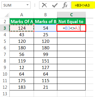
Step 2: Press the “Enter” key. The output in cell C3 is “true.” This is shown in the following image.

Step 3: Drag the formula of cell C3 till cell C12 by using the fill handle. This is shown in the following image.

Step 4: The outputs for the entire column C are shown in the following image. The outputs which are false have been colored yellow. The inferences from this dataset are stated as follows:

If the output is “true,” the values of column A and column B for a given row are not equal. This means that the “not equal to” excel condition for that particular row is met. For instance, the “not equal to” condition for row 3 is “=B3<>A3.” In other words, 124 is not equal to 54.
If the output is “false,” the values of column A and column B for a given row are equal. This means that the “not equal to” condition for that particular row is not met. For instance, the “not equal to” condition for row 5 is “=B5<>A5.” In other words, 120 is certainly equal to 120.

Overall, for three rows (rows 5, 6, and 10), the marks of students A and B are equal. Except for these rows, the marks are unequal in all the remaining rows (rows 3, 4, 7, 8, 9, 11, and 12). Without knowing the magnitude of difference, one cannot conclude whose performance (from students A and B) is better.

Example #2–Compare two Textual Values with the “Not Equal To” Operator

In the dataset of example #1, we have substituted random grades (from A to J) in place of numbers. We want to find the rows for which the grades of students A and B are unequal. Use the “not equal to” operator of Excel.

The steps to find if a difference exists (between the grades) are listed as follows:

Step 1: Enter the formula “=B3<>A3” in cell C3. Press the “Enter” key. The output in cell C3 is “true.” So, for row 3, the “not equal to” excel operator has validated that the values in the first and second cell (A3 and B3) are not equal.

Step 2: Drag the formula of cell C3 till cell C12. The outputs for the entire column C are shown in the following image. The single false output has been colored yellow.

The output in cell C3 meets the “not equal to” excel condition, which is “=B3<>A3.” In contrast, the output in cell C11 does not meet the “not equal to” condition, which is “=B11<>A11.” Hence, the grades of all rows, except row 11, are unequal. The grades of the two students are equal for row 11.

Example #3–Obtain Defined Results with the IF Function and the “Not Equal To” Condition

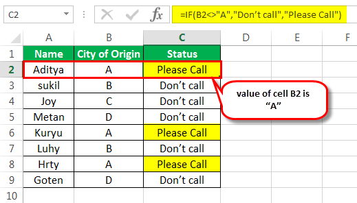
The succeeding image shows the names of a few candidates and their native places in columns A and B respectively. From these candidates, an organization wants to hire those candidates whose city of origin is “A.”

We want to differentiate candidates who need to be contacted and who need not be contacted for the further hiring process. For this, display the status as either “please call” or “don’t call” (in column C), depending on whether the hometown of a candidate is “A” or not.

Use the IF function and the “not equal to” operator of Excel.

The steps to use the IF functionIF function in Excel evaluates whether a given condition is met and returns a value depending on whether the result is “true” or “false”. It is a conditional function of Excel, which returns the result based on the fulfillment or non-fulfillment of the given criteria.
read more and the “not equal to” operator are listed as follows:

Step 1: Enter the following formula in cell C2.

“=IF(B2<>”A”,”Don’t call”,”Please Call”)”

Press the “Enter” key. Drag the formula till cell C9. The outputs of column C are shown in the succeeding image. The candidates whose city of origin is “A” have been assigned the “please call” status in column C.

Note: In the given IF formula, the condition [B2<>“A”] is the logical test. The string “don’t call” is “value_if_true” and the string “please call” is “value_if_false.”

So, the IF formula returns “don’t” call” for a given row, if the value of column B is not equal to “A” (i.e., the condition is true). It returns “please call” for a given row, if the value of column B is equal to “A” (i.e., the condition is false).

With the help of the IF function, Excel can display different results for the matched and unmatched conditions. For more details related to the IF function of Excel, click the hyperlink given immediately before step 1 of this example.

Step 2: The candidates whose hometown is other than “A” have been assigned the “don’t call” status in column C. This is shown in the following image.

Hence, only candidates “Aditya,” “Kuryu,” and “Hrty” should be called for the further round of interviews. The remaining candidates need not be contacted.

So, with the IF function and the “not equal to” excel operator, we have successfully differentiated the candidates who can be hired from those who cannot be hired.

Note: Notice that this step has been added only for the purpose of understanding. The preceding step (step 1) is complete in itself for the given task of hiring candidates.

Example #4–Count Specific Cells with the COUNTIF Function and the “Not Equal To” Condition

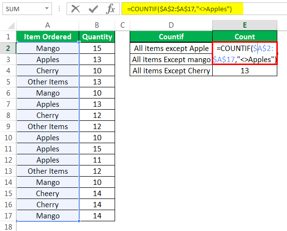
The succeeding image shows certain fruits (or items) in column A and their quantities ordered in column B. Apart from apples, mangoes, and cherries, the remaining fruits have been clubbed under “other items” in column A.

We want to count the number of cells (of column A) that are not equal to:

“Apples”
“Mango”
“Cherry”

There should be three outputs, one output excluding one fruit. Use the COUNTIF function and the “not equal to” operator of Excel.

The steps to use the COUNTIF functionThe COUNTIF function in Excel counts the number of cells within a range based on pre-defined criteria. It is used to count cells that include dates, numbers, or text. For example, COUNTIF(A1:A10,”Trump”) will count the number of cells within the range A1:A10 that contain the text “Trump”
read more and the “not equal to” operator are listed as follows:

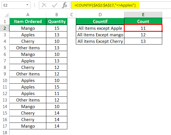
Step 1: Enter the following formulas in cells E2, E3, and E4 respectively.

“=COUNTIF($A$2:$A$17,”<>Apples”)”
“=COUNTIF($A$2:$A$17,”<>Mango”)”
“=COUNTIF($A$2:$A$17,”<>Cherry”)”

Press the “Enter” key after entering each formula.

The first formula counts the number of cells in the range A2:A17, which do not contain the string “apples.” Likewise, the second formula counts the number of cells in this range that do not contain the string “mango.” The third formula helps count the number of cells in the given range (A2:A7), which do not contain the string “cherry.”

Notice that the succeeding image shows the formula in cell E2 and the result of the third formula in cell E4.

Note: “$A$2:$A$17” is the “range” argument of the preceding COUNTIF formulas. The condition “<>Apples” is the “criteria” argument of the first formula. In all the preceding formulas, the range is the same, but the criterions are different.

The COUNTIF counts the cells of a range, which satisfy a single criterion. For more details related to the COUNTIF function, click the hyperlink given before step 1 of this example.

Step 2: The following image shows the three outputs (in cells E2, E3, and E4) of the three formulas entered in the preceding step.

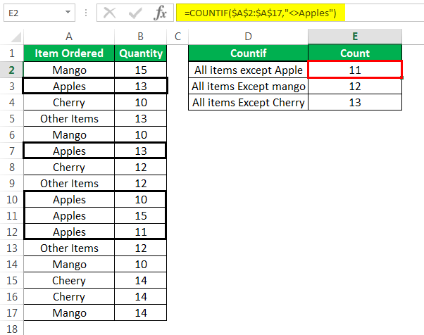
Notice that “cherry” has been deliberately misspelled as “cheery” in cell A15. As a result, this cell has also been counted (as a cell not containing “cherry”) by the third COUNTIF formula.

Had the word been correctly spelled in cell A15, the output in cell E4 would have been 12. In this case, cell A15 would have been excluded from the count (as a cell containing “cherry”).

Step 3: The rows containing “apples” are displayed in black boxes in the following image. These rows are excluded while counting the cells not containing “apples.” Hence, 11 cells (in the range A2:A17) do not contain the string “apples.”

Likewise, in the given range, 12 cells do not contain the string “mango” and 13 cells do not contain the string “cherry.”

Note: This step has been added only for notifying the readers, the cells that are counted and the cells that are left out by the first COUNTIF formula (entered in step 1).

Example #5–Sum Particular Cells with the SUMIF Function and the “Not Equal To” Condition

Working on the data of example #3, we want to sum the quantities of column B that are not equal to:

“Apples”
“Mango”
“Cherry”

There should be three summed outputs where each output excludes one fruit. Use the SUMIF function and the “not equal to” sign of Excel.

The steps to use the SUMIF functionThe SUMIF Excel function calculates the sum of a range of cells based on given criteria. The criteria can include dates, numbers, and text. For example, the formula “=SUMIF(B1:B5, “<=12”)” adds the values in the cell range B1:B5, which are less than or equal to 12.
read more and the “not equal to” operator are listed as follows:

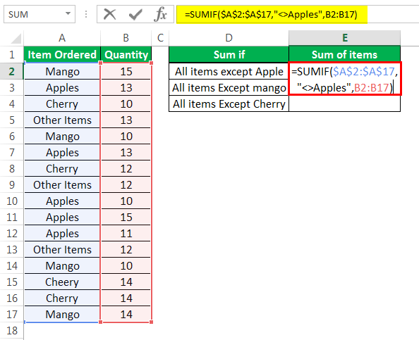
Step 1: Enter the following formulas in cells E2, E3, and E4 respectively.

“=SUMIF($A$2:$A$17,”<>Apples”,B2:B17)”
“=SUMIF($A$2:$A$17,”<>Mango”,B2:B17)”
“=SUMIF($A$2:$A$17,”<>Cherry”,B2:B17)”

The first formula is shown in the following image.

In all three formulas, the SUMIF function evaluates the range A2:A17. For cells not equal to “apples” (in range A2:A17), the first formula sums the numbers of the range B2:B17. Likewise, for cells not equal to “mango” in the given range (A2:A17), the second formula also sums the numbers of the range B2:B17. Similar summing is carried out by excluding cells containing “cherry.”

Note: “$A$2:$A$17” is the “range” argument of the SUMIF function. The condition “<>Apples” is the “criteria” argument. The range “B2:B17” is the “sum_range” argument of the SUMIF function.

With the SUMIF function, we have applied the given condition (in each formula) to the range A2:A17 and summed up the corresponding values of the range B2:B17. Usually, the SUMIF works with a single criterion. For more details related to the SUMIF function, click the hyperlink given before step 1 of this example.

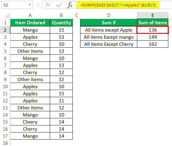
Step 2: Press the “Enter” key after entering each of the preceding formulas. The three summed outputs are shown in the following image.

Hence, the sum of all the fruit quantities except “apples” is 136. Excluding the cells containing “mango,” this sum is 149. Likewise, leaving the cells containing “cherry,” this sum is 162.

Notice that the value of cell B15 has also been included in the sum returned (in cell E4) by the third SUMIF formula (entered in step 1). This is because in cell A15, the spelling of “cherry” has been misspelled as “cheery.” Hence, Excel considers A15 as a cell not containing “cherry.”

The important points governing the usage of the “not equal to” operator of Excel are listed as follows:

The “not equal to” is the converse of the “equal to” operator. This implies that the interpretation of “true” and “false” is exactly the opposite with these two logical operators.
The results produced by the “not equal to” operator are similar to those returned by the NOT function of Excel. The NOT function reverses the “true” and “false” outcomes of a condition. For instance, if the output of a condition is “false,” the formula “=NOT(false)” returns “true.”
The “not equal to” operator is case-insensitive. This means that it ignores the casing of the two text strings that are compared. For instance, if “rose” and “ROSE” are compared using the “not equal to” operator, the output is “false.” This is because these two values mean the same to the “not equal to” excel operator.

Frequently Asked Questions

1. Define the “not equal to” operator and state how is it used in Excel.

The “not equal to” excel operator checks whether two values (numeric or textual) being compared are different from each other or not. If the values are different, the output is “true.” If the values are the same, the output is “false.” The “not equal to” operator is the easiest method to ensure that a difference exists between two values.

In Excel, the “not equal to” operator is used as follows:

“=value1<>value2”

“Value1” is the first value to be compared and “value2” is the second value to be compared.

Note: Exclude the beginning and ending double quotation marks while entering the “not equal to” condition in Excel. For more details related to the usage of this operator, refer to the examples of this article.

2. How to use the “not equal to” operator with the conditional formatting feature of Excel?

The steps to use the “not equal to” with the conditional formatting feature of Excel are listed as follows:

a. Select the range on which a conditional formatting rule is to be applied.
b. From the Home tab, click the “conditional formatting” drop-down from the “styles” group. Next, click “new rule.”
c. The “new formatting rule” window opens. Under “select a rule type,” choose the option “use a formula to determine which cells to format.”
d. Under “format values where this formula is true,” enter the desired formula. For instance, if cells (in the range A1:A6) not equal to 2 are to be formatted, enter the formula as “=A1<>2” (without the beginning and ending double quotation marks).
e. Click “format” and select a color from the “fill” tab. Click “Ok” in the “format cells” window.
f. Click “Ok” again in the “new formatting rule” window.

The chosen color (selected in step “e”) is applied to the selected range (selected in step “a”). If the formula given in step “d” is applied, the cells of the range A1:A6, which do not contain 2, are colored. No formatting is applied to the remaining cells.

Note: To conditionally format a range of text values by using the “not equal to” operator, keep the string of the formula in double quotation marks. For instance, the formula [=A1<>“rose”] formats those cells of the selected range which do not contain the string “rose.” Exclude the beginning and ending square brackets while applying this formula.

3. How to use the “not equal to” operator to find blanks in a range of Excel?

The steps to find blanks in Excel by using the “not equal to” operator are listed as follows:

a. Enter the formula containing the cell reference (to be evaluated), “not equal to” operator, and an empty text string. For instance, if blanks in the range A1:A6 are to be found, enter the formula =A1<>“” in cell B1.
b. Press the “Enter” key. Drag the formula to the remaining range (of column B) to obtain outputs for the entire column (column A).

The cells containing blanks have been identified. The formula entered in step “a” returns “true” for all values which are not blanks. For all blank values, this formula returns “false.”

Since the double quotation marks of the formula represent an empty string, a “false” implies that the cell value is equal to an empty string. Conversely, a “true” implies that the cell contains some value, which is not equal to an empty string.

Example 1

Figure 1. Setting the data

This data refers to the total and obtained GPA of students. Only those students will be selected for scholarship that got 4 out of 4 GPA.

We need to use conditional formatting to highlight the students with a GPA less than 4 in order to avoid them for selection.

Or we can say, we need to highlight the cells of Column C and F that are not equal to the cells of Column B and E.

Steps

Select cells of column C from C2 to C14.

Select conditional formatting in the “Styles” section of the toolbar.

Click the option of “New Rule” and “New formatting Rule” window will appear.

Choose the rule type written as “Use a formula to determine which cells to format” from window.

In order to write the formula in the “Rule Description” bar, Select cell C2 to C14, put a “Not Equal to” sign and then select cells from B2 to B14.

(The sign <> is referred as “Not Equal to” sign in Excel)

Now click on the ‘format” option to select format of your choice like color of the formatted cells etc.

Figure 2. Applying formatting rule for example 1

“New Formatting Rule” window will appear like this. Press OK to apply conditional formatting.

Do the same with Column F and the unequal cells will appear highlighted as given in the figure below.

Figure 3. Result of example 1

Example 2

Figure 4. Applying formatting rule for example 2

This is another example of conditional formatting where cells are not equal.

In this example, we’ll apply conditional formatting in order to highlight the boxes with unequal length and width.

We can separate unequal boxes from the boxes of equal measurements with the help of conditional formatting.

Same process and formula from Example # 1 is followed in Example # 2 and the final figure is given below.

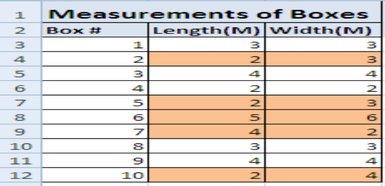Figure 5. Result of example 2

Note

The formula is automatically locked in the rule description section and appears like this:

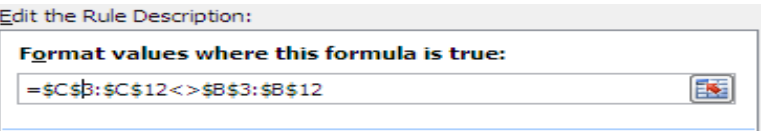Figure 6. Formula

Remove the $ sign before the number of rows/numerical figures to get accurate results.

Most of the time, the problem you will need to solve will be more complex than a simple application of a formula or function. If you want to save hours of research and frustration, try our live Excelchat service! Our Excel Experts are available 24/7 to answer any Excel question you may have. We guarantee a connection within 30 seconds and a customized solution within 20 minutes.

Источник

Testing whether conditions are true or false and making logical comparisons between expressions are common to many tasks. You can use the AND, OR, NOT, and IF functions to create conditional formulas.

For example, the IF function uses the following arguments.

Formula that uses the IF function

logical_test: The condition that you want to check.

value_if_true: The value to return if the condition is True.

value_if_false: The value to return if the condition is False.

For more information about how to create formulas, see Create or delete a formula.

What do you want to do?

Create a conditional formula that results in a logical value (TRUE or FALSE)
Create a conditional formula that results in another calculation or in values other than TRUE or FALSE

Create a conditional formula that results in a logical value (TRUE or FALSE)

To do this task, use the AND, OR, and NOT functions and operators as shown in the following example.

Example

The example may be easier to understand if you copy it to a blank worksheet.

How do I copy an example?

Select the example in this article.

Selecting an example from Help
Press CTRL+C.
In Excel, create a blank workbook or worksheet.
In the worksheet, select cell A1, and press CTRL+V.

Important: For the example to work properly, you must paste it into cell A1 of the worksheet.

To switch between viewing the results and viewing the formulas that return the results, press CTRL+` (grave accent), or on the Formulas tab, in the Formula Auditing group, click the Show Formulas button.

After you copy the example to a blank worksheet, you can adapt it to suit your needs.

Data
15
9
8
Sprockets
Widgets
Formula	Description (Result)
=AND(A2>A3, A2<A4)	Determines if the value in cell A2 is greater than the value in A3 and also if the value in A2 is less than the value in A4. (FALSE)
=OR(A2>A3, A2<A4)	Determines if the value in cell A2 is greater than the value in A3 or if the value in A2 is less than the value in A4. (TRUE)
=NOT(A2+A3=24)	Determines if the sum of the values in cells A2 and A3 is not equal to 24. (FALSE)
=NOT(A5=»Sprockets»)	Determines if the value in cell A5 is not equal to «Sprockets.» (FALSE)
=OR(A5<>»Sprockets»,A6 = «Widgets»)	Determines if the value in cell A5 is not equal to «Sprockets» or if the value in A6 is equal to «Widgets.» (TRUE)

For more information about how to use these functions, see AND function, OR function, and NOT function.

Top of Page

Create a conditional formula that results in another calculation or in values other than TRUE or FALSE

To do this task, use the IF, AND, and OR functions and operators as shown in the following example.

Example

The example may be easier to understand if you copy it to a blank worksheet.

How do I copy an example?

Select the example in this article.

Important: Do not select the row or column headers.

Selecting an example from Help
Press CTRL+C.
In Excel, create a blank workbook or worksheet.
In the worksheet, select cell A1, and press CTRL+V.

Important: For the example to work properly, you must paste it into cell A1 of the worksheet.

To switch between viewing the results and viewing the formulas that return the results, press CTRL+` (grave accent), or on the Formulas tab, in the Formula Auditing group, click the Show Formulas button.

After you copy the example to a blank worksheet, you can adapt it to suit your needs.

Data
15
9
8
Sprockets
Widgets
Formula	Description (Result)
=IF(A2=15, «OK», «Not OK»)	If the value in cell A2 equals 15, return «OK.» Otherwise, return «Not OK.» (OK)
=IF(A2<>15, «OK», «Not OK»)	If the value in cell A2 is not equal to 15, return «OK.» Otherwise, return «Not OK.» (Not OK)
=IF(NOT(A2<=15), «OK», «Not OK»)	If the value in cell A2 is not less than or equal to 15, return «OK.» Otherwise, return «Not OK.» (Not OK)
=IF(A5<>»SPROCKETS», «OK», «Not OK»)	If the value in cell A5 is not equal to «SPROCKETS», return «OK.» Otherwise, return «Not OK.» (Not OK)
=IF(AND(A2>A3, A2<A4), «OK», «Not OK»)	If the value in cell A2 is greater than the value in A3 and the value in A2 is also less than the value in A4, return «OK.» Otherwise, return «Not OK.» (Not OK)
=IF(AND(A2<>A3, A2<>A4), «OK», «Not OK»)	If the value in cell A2 is not equal to A3 and the value in A2 is also not equal to the value in A4, return «OK.» Otherwise, return «Not OK.» (OK)
=IF(OR(A2>A3, A2<A4), «OK», «Not OK»)	If the value in cell A2 is greater than the value in A3 or the value in A2 is less than the value in A4, return «OK.» Otherwise, return «Not OK.» (OK)
=IF(OR(A5<>»Sprockets», A6<>»Widgets»), «OK», «Not OK»)	If the value in cell A5 is not equal to «Sprockets» or the value in A6 is not equal to «Widgets», return «OK.» Otherwise, return «Not OK.» (Not OK)
=IF(OR(A2<>A3, A2<>A4), «OK», «Not OK»)	If the value in cell A2 is not equal to the value in A3 or the value in A2 is not equal to the value in A4, return «OK.» Otherwise, return «Not OK.» (OK)

For more information about how to use these functions, see IF function, AND function, and OR function.

Top of Page

Источник

Explanation

Increase price if color NOT red or green

What is “Not Equal To” Sign in Excel?

Table of contents

How is the “Not Equal To” Sign Used in Excel?

Example #1–Compare two Numeric Values with the “Not Equal To” Operator

Example #2–Compare two Textual Values with the “Not Equal To” Operator

Example #3–Obtain Defined Results with the IF Function and the “Not Equal To” Condition

Example #4–Count Specific Cells with the COUNTIF Function and the “Not Equal To” Condition

Example #5–Sum Particular Cells with the SUMIF Function and the “Not Equal To” Condition

Frequently Asked Questions

Recommended Articles

Example 1

Steps

Example 2

Note

What do you want to do?

Create a conditional formula that results in a logical value (TRUE or FALSE)

Example

Create a conditional formula that results in another calculation or in values other than TRUE or FALSE

Example