
I get this query all the time. People have huge data sets and someone in their team has highlighted some records by formatting it in bold font.
Now, you are the one who gets this data, and you have to filter all these records that have a bold formatting.
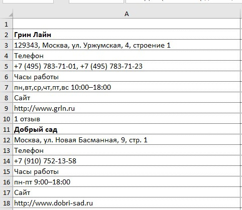
For example, suppose you have the data set as shown below, and you want to filter all the cells that have been formatted in bold font.

Let’s face it.
There is no straightforward way of doing it.
You cannot simply use an Excel filter to get all the bold cells. But that doesn’t mean you have to waste hours and do it manually.
In this tutorial, I will show you three ways to filter cells with bold font formatting in Excel:

Method 1 – Filter Bold Cells Using Find and Replace
Find and Replace can be used to find specific text in the worksheet, as well as a specific format (such as cell color, font color, bold font, font color).
The idea is to find the bold font formatting in the worksheet and convert it into something that can be easily filtered (Hint: Cell color can be used as a filter).
Here are the steps filter cells with bold text format:
- Select the entire data set.
- Go to the Home tab.
- In the Editing group, click on the Find and Select drop down.
- Click on Replace. (Keyboard shortcut: Control + H)

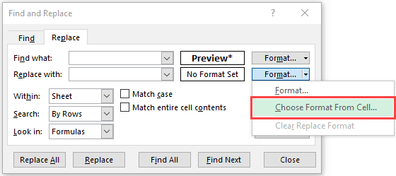
- In the Find and Replace dialog box, click on the Options button.

- In the Find what section, go to the Format drop-down and select ‘Choose Format From Cell’.
- Select any cell which has the text in bold font format.

- In the ‘Replace with:’ section, go to Format drop-down and click on ‘Choose Format From Cell’ option.

- In the Replace Format dialog box, select the Fill Tab and select any color and click OK (make sure it’s a color that is not there already in your worksheet cells).
- Click on Replace All. This will color all the cells that have the text with bold font formatting.


In the above steps, we have converted the bold text format into a format that is recognized as a filter criterion by Excel.
Now to filter these cells, here are the steps:
- Select the entire data set.
- Go to the Data tab.
- Click on the Filter icon (Key Board Shortcut: Control + Shift + L)
- For the column that you want to filter, click on the filter icon (the downward pointing arrow in the cell).
- In the drop-down, go to the ‘Filter by Color’ option and select the color you applied to cells with text in bold font format.

This will automatically filter all those cells that have bold font formatting in it.
Try it yourself.. Download the file

Method 2 – Using Get.Cell Formula
It time for a hidden gem in Excel. It’s an Excel 4 macro function – GET.CELL().
This is an old function which does not work in the worksheet as regular functions, but it still works in named ranges.
GET.CELL function gives you the information about the cell.
For example, it can tell you:
- If the cell has bold formatting or not
- If the cell has a formula or not
- If the cell is locked or not, and so on.
Here is the syntax of the GET.CELL formula
=GET.CELL(type_num, reference)
- Type_num is the argument to specify the information that you want to get for the referenced cell (for example, if you enter 20 as the type_num, it would return TRUE if the cell has a bold font format, and FALSE if not).
- Reference is the cell reference that you want to analyze.
Now let me show you how to filter cells with text in a bold font format using this formula:
- Go to Formulas tab.
- Click on the Define Name option.
- In the New Name dialog box, use the following details:
- Name: FilterBoldCell
- Scope: Workbook
- Refers to: =GET.CELL(20,$A2)
- Click OK.
- Go to cell B2 (or any cell in the same row as that of the first cell of the dataset) and type =FilterBoldCell
- Copy this formula for all the cell in the column. It will return a TRUE if the cell has bold formatting and FALSE if it does not.
- Now select the entire data set, go to the Data tab and click on the Filter icon.
- In the column where you have TRUE/FALSE, select the filter drop-down and select TRUE.


That’s it!
All the cells with text in bold font format have now been filtered.
Note: Since this is a macro function, you need to save this file with a .xlsm or .xls extension.
I could not find any help article on GET.CELL() by Microsoft. Here is something I found on Mr. Excel Message Board.
Try it yourself.. Download the file
Method 3 – Filter Bold Cells using VBA
Here is another way of filtering cells with text in bold font format by using VBA.
Here are the steps:
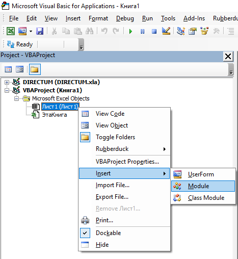
- Right-click on the worksheet tab and select View Code (or use the keyboard shortcut ALT + F11). This opens the VB Editor backend.

- In the VB Editor window, there would be the Project Explorer pane. If it is not there, go to View and select Project Explorer.
- In the Project Explorer pane, right click on the workbook (VBAProject) on which you are working, go to Insert and click on Module. This inserts a module where we will put the VBA code.

- Double click on the module icon (to make sure your code into the module), and paste the following code in the pane on the right:
Function BoldFont(CellRef As Range)
BoldFont = CellRef.Font.Bold
End Function
- Go to the worksheet and use the below formula: =BoldFont(B2)
- This formula returns TRUE wherever there is bold formatting applied to the cell and FALSE otherwise. Now you can simply filter all the TRUE values (as shown in Method 2)


Again! This workbook now has a macro, so save it with .xlsm or .xls extension
Try it yourself.. Download the file
I hope this will give you enough time for that much-needed coffee break 🙂
Do you know any other way to do this? I would love to learn from you. Leave your thoughts in the comment section and be awesome.
You May Also Like the Following Excel Tutorials:
- An Introduction to Excel Data Filter Options.
- Filter By Color in Excel
- Create Dynamic Excel Filter – Extract Data as you type.
- Creating a Drop Down Filter to Extract Data Based on Selection.
- Filter the Smart Way – Use Advanced Filter in Excel
- Count Cells Based on a Background Color.
- Highlight Blank Cells in Excel.
- How to Create a Heat Map in Excel.
- Excel VBA Autofilter.
Набросок.
Sub test_()
    Dim aData(), rRng As Range
    Dim i As Long, k As Long

    With ActiveSheet ' лист с исходными данными'
        i = .Cells(.Rows.Count, 1).End(xlUp).Row ' последняя строка с данными'
        Set rRng = .Range("A1:A" & i).Value ' диапазон в переменную, для отслеживания форматирования'
    End With

    aData = rRng.Value ' для ускорения чтения данные заносим в массив'
    ReDim aRes(1 To i, 1 To 6) ' 6 - количество столбцов (количество нужных данных из одного блока данных)'

    For i = 2 To UBound(aData)
        If rRng(i, 1).Font.Bold = True Then
            k = k + 1 ' номер записи в массиве выгрузки'
            aRes(k, 1) = aData(i, 1)
            ' здесь получить другие данные блока'
        End If
    Next i

    ' Worksheets("2") ' лист для выгрузки результата'
    Worksheets("2").Range("A2").Resize(UBound(aRes), UBound(aRes, 2)).Value = aRes
    Set rRng = Nothing
End Sub
Т.к. «другие поля (телефон, часы работы и сайт) есть не у всех данных«, то для получения других данных из блока нужно отслеживать наполнение блока.
Если нужно получить только жирные заголовки блоков, то массив выгрузки можно ограничить одним столбцом.

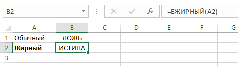
Как найти значения ячеек с жирным шрифтом?
Нужно выбрать значения ячеек для копирования на другой лист документа, привязавшись к ячейке с жирным шрифтом. На одном сайте нашел такую формулу: =ЕЖИРНЫЙ(А2), но у меня в excel нет такой формулы. Как можно сделать?
-
Вопрос заданболее года назад
-
513 просмотров
Попробуйте почитать информацию на сайте до конца, там ниже будет:
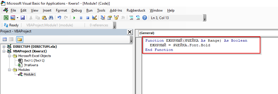
Function ЕЖИРНЫЙ(ЯЧЕЙКА As Range) As Boolean
  ЕЖИРНЫЙ = ЯЧЕЙКА.Font.Bold
End Function
upd
1. Открываете файл Excel
2. Нажимаете Alt+F11
3. Создаете новый модуль
spoiler
4. Вставляете код
spoiler
5. И далее пользуетесь как обычной формулой
spoiler
Пригласить эксперта
-
Показать ещё
Загружается…
14 апр. 2023, в 01:55
1000 руб./в час
13 апр. 2023, в 23:50
3000 руб./за проект
13 апр. 2023, в 23:18
1000 руб./за проект
Минуточку внимания
![]()
Written by Allen Wyatt (last updated February 1, 2020)
This tip applies to Excel 2007, 2010, 2013, 2016, 2019, and Excel in Microsoft 365
Ken wonders if there is a worksheet function that will indicate whether the contents of a cell are bold. He can find other informational functions, such as ISBLANK, but cannot find one that will indicate if the cell is bold.
There is no ISBOLD function built into Excel. There is a very arcane way to do this without resorting to a macro, but it only works with some versions of Excel. Apparently, for example, this approach won’t work with Office 365, as it appears that Microsoft has finally removed support for it. This old Excel 4 function, called GET.CELL, will work with some older versions of Excel. Here is how you would use it in a formula:
=IF(GET.CELL(20,A1), "Bold", "Not Bold")
The GET.CELL function returns True if at least the first character in the cell is bold.
A better approach would be to create a User-Defined Function in VBA that could be called from your worksheet. Here’s a simple version of such a UDF:
Function CheckBold(cell As Range) As Boolean
    Application.Volatile
    CheckBold = cell.Font.Bold
End Function
In order to use it in your worksheet, you would do so in this manner:
=IF(CheckBold(A1), "Bold", "Not Bold")
The CheckBold function will only update when your worksheet is recalculated, not if you simply apply bold formatting to or remove it from cell A1.
This approach can work for most instances but understand that the Bold property can actually have three possible settings—True, False, and Null. The property is set to False if none of the characters in the cell are bold. It is set to True if they are all bold. Finally, it is set to Null if only some of the characters in the cell are bold. If you think you might run into this situation, then you’ll need to modify the CheckBold function:
Function CheckBold(cell As Range) As Integer
    Dim iBold As Integer

    Application.Volatile

    iBold = 0
    If IsNull(cell.Font.Bold) Then
        iBold = 2
    Else
        If cell.Font.Bold Then iBold = 1
    End If

    CheckBold = iBold
End Function
Note that the function now returns a value, 0 through 2. If it returns 0, there is no bold in the cell. If it returns 1, then the entire cell is bold. If it returns 2, then there is partial bold in the cell.
If you would like to know how to use the macros described on this page (or on any other page on the ExcelTips sites), I’ve prepared a special page that includes helpful information. Click here to open that special page in a new browser tab.
ExcelTips is your source for cost-effective Microsoft Excel training.
This tip (13733) applies to Microsoft Excel 2007, 2010, 2013, 2016, 2019, and Excel in Microsoft 365.
Author Bio
With more than 50 non-fiction books and numerous magazine articles to his credit, Allen Wyatt is an internationally recognized author. He is president of Sharon Parq Associates, a computer and publishing services company. Learn more about Allen…
MORE FROM ALLEN
Determining a State from an Area Code
Want to be able to take information that is in one cell and match it to data that is contained in a table within a …
Discover More
Editing a Comment Close to Its Cell
Have you ever chosen to edit a comment, only to find that the comment is quite a ways from the cell with which it is …
Discover More
Using Subtotals and Totals
You can insert subtotals and totals in your worksheets by using either a formula or specialized tools. This tip explains …
Discover More
-
#2
In VBA you can; not so sure about a formula solution….
-
#3
The short answer is yes.
The long answer is, yes but it depends on how your cells got bolded.
If the bold format is due to the cell’s font property being set to «Bold» (such as when you click on Format > Cells > Font Tab) then
You will need a user defined function in VBA to construct a formula to identify the bold property.
Otherwise if the font is bold due to conditional formatting then
you can get by with a formula that tests for the same condition in the subject cell as does the conditional formatting.
So, clarify what you really have and someone can assist with a formula that is appropriate for your situation.
-
#4
Hi,
| PivotTest.xls | ||||
|---|---|---|---|---|
|
|
||||
| A | B | C | D | |
| 1 | a | 0 | ||
| 2 | b | 1 | ||
| 3 | c | 0 | ||
| 4 | d | 1 | ||
| 5 | e | 0 | ||
| 6 | f | 1 | ||
| 7 | g | 0 | ||
| 8 | h | 1 | ||
| 9 | I | 0 | ||
| 10 | j | 1 | ||
|
Sheet2 |
Bold defined as
=GET.CELL(20,Sheet2!$A1)
HTH
-
#5
The formatting is not conditional — hopefully this will make the answer easier
-
#6
You will have to do a Recalc (F9) if you change the bolding for it to update after changes, but perhaps:
Code:
Public Function isbold(r As Range) As Integer
Application.Volatile
isbold = Abs(r.Font.Bold = True)
End Function