
After checking if a cell value exists in a column, I need to get the value of the cell next to the matching cell. For instance, I check if the value in cell A1 exists in column B, and assuming it matches B5, then I want the value in cell C5.
To solve the first half of the problem, I did this…
=IF(ISERROR(MATCH(A1,B:B, 0)), "No Match", "Match")
…and it worked. Then, thanks to an earlier answer on SO, I was also able to obtain the row number of the matching cell:
=IF(ISERROR(MATCH(A1,B:B, 0)), "No Match", "Match on Row " & MATCH(A1,B:B, 0))
So naturally, to get the value of the next cell, I tried…
=IF(ISERROR(MATCH(A1,B:B, 0)), "No Match", C&MATCH(A1,B:B, 0))
…and it doesn’t work.
What am I missing? How do I append the column number to the row number returned to achieve the desired result?
This post will guide you how to check if one value in a column exists in another column in Excel. How do I check if value in column A exists in Column B with a formula in Excel. How to determine if values exists in another column in Excel.
Table of Contents
- Check If Value in a Column exists in Another Column
- Related Functions
Assuming that you have a list of data in two columns in range A1:B5, and you want to check if one value in column A exists in column B, if True, then return true, otherwise, returns False. How to achieve it. You can create a new formula based on the IF function, the ISERROR function and the VLOOKUP function. Like this:
=IF(ISERROR(VLOOKUP(A1,$B$1:$B$5, 1, FALSE)),FALSE,TRUE )
Type this formula into cell C1, and press Enter key in your keyboard, and then drag the autofill handle over other cells to apply this formula to check other cells in Column A.
- Excel IF function
The Excel IF function perform a logical test to return one value if the condition is TRUE and return another value if the condition is FALSE. The IF function is a build-in function in Microsoft Excel and it is categorized as a Logical Function.The syntax of the IF function is as below:= IF (condition, [true_value], [false_value])…. - Excel VLOOKUP function
The Excel VLOOKUP function lookup a value in the first column of the table and return the value in the same row based on index_num position.The syntax of the VLOOKUP function is as below:= VLOOKUP (lookup_value, table_array, column_index_num,[range_lookup])…. - Excel ISERROR function
The Excel ISERROR function used to check for any error type that excel generates and it returns TRUE for any error type, and the ISERR function also can be checked for error values except #N/A error, it returns TRUE while the error is #N/A. The syntax of the ISERROR function is as below:= ISERROR (value)….
When you need to check if one column value exists in another column in Excel, there are several options. One of the most important features in Microsoft Excel is lookup and reference. The VLOOKUP, HLOOKUP, INDEX and MATCH functions can make life a lot easier in terms of looking for a match.
In this tutorial, we will see the use of VLOOKUP and INDEX/MATCH to check if one values from one column exist in another column.
Check if one column value exists in another column
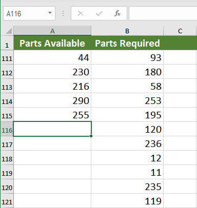
In the following example, you will work with automobile parts inventory data set. Column A has the parts available, and column B has all the parts needed. Column A has 115 entries, and column B has 1001 entries. We will discuss a couple of ways to match the entries in column A with the ones in column B. Column C will output “True” if there is a match, and “False” if there isn’t.
Check if one column value exists in another column using MATCH
You can use the MATCH() function to check if the values in column A also exist in column B. MATCH() returns the position of a cell in a row or column. The syntax for MATCH() is =MATCH(lookup_value, lookup_array, [match_type]). Using MATCH, you can look up a value both horizontally and vertically.
Example using MATCH
To solve the problem in the previous example with MATCH(), you need to follow the following steps:
- Select cell C2 by clicking on it.
- Insert the formula in
"=NOT(ISERROR(MATCH(A2,$B$2:$B$1001,0)))”the formula bar. - Press Enter to assign the formula to C2.

- Drag the formula down to the other cells in column C clicking and dragging the little “+” icon on the bottom-right of C2.
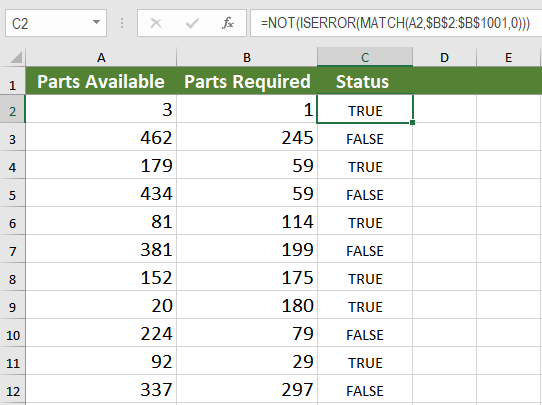
Excel will match the entries in column A with the ones in column B. If there is a match, it will return the row number. The NOT() and ISERROR() functions check for an error which would be and column C will show “True” for a match and “False” if it is not a match.
Check if one column value exists in another column using VLOOKUP
VLOOKUP is one of the lookup, and reference functions in Excel and Google Sheets used to find values in a specified range by “row.” It compares them row-wise until it finds a match. In this tutorial, we will look at how to use VLOOKUP on multiple columns with multiple criteria. The syntax for VLOOKUP is =VLOOKUP(value, table_array, col_index,[range_lookup]).
Example using VLOOKUP
You can check if the values in column A exist in column B using VLOOKUP.
- Select cell C2 by clicking on it.
- Insert the formula in
“=IF(ISERROR(VLOOKUP(A2,$B$2:$B$1001,1,FALSE)),FALSE,TRUE)”the formula bar. - Press Enter to assign the formula to C2.
- Drag the formula down to the other cells in column C clicking and dragging the little “+” icon on the bottom-right of C2.
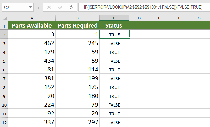
This will allow Excel to look up all the values in column A and match them with the values of column B. Column C will now show “True” if the corresponding cell in column A has a match in column B, “False” if it does not have a match.
MATCH vs. VLOOKUP – Which is Better?
Between MATCH and VLOOKUP, the better option is MATCH. Not only the formula is simpler, but MATCH is also faster than VLOOKUP when it comes to performance.
MATCH uses a dynamic column reference whereas VLOOKUP uses a static one. If you were to add more columns, with VLOOKUP, you would distort the results. But with MATCH you can easily change the reference when inserting or deleting columns.
Another issue with VLOOKUP is that the lookup value needs to be on the leftmost column of the array, which is not applicable for MATCH. In the previous example, If we had to check if Column C values exist in column A, VLOOKUP would have provided an #N/A error.
Excel has some very effective functions when it comes to checking if values in one column exist in another column. One of these functions is MATCH. It returns the row number based on the lookup value from an array. Another such function is VLOOKUP. It returns the value based on a lookup value from a static array.
When it comes to which function is faster, MATCH is the winner. For its dynamic reference and easy to change array references, MATCH is preferred to check if values in one column also exist in another column.
Most of the time, the problem you need is probably more complex than just simply checking if a value exists in a column. If you want to save hours of researching and frustration, try our Excel Live Chat service! Our Excel experts are available 24/7 to answer any Excel question you have on the spot. The first question is free.
Are you still looking for help with the VLOOKUP function? View our comprehensive round-up of VLOOKUP function tutorials here.
In this example, the goal is to use a formula to check if a specific value exists in a range. The easiest way to do this is to use the COUNTIF function to count occurences of a value in a range, then use the count to create a final result.
COUNTIF function
The COUNTIF function counts cells that meet supplied criteria. The generic syntax looks like this:
=COUNTIF(range,criteria)Range is the range of cells to test, and criteria is a condition that should be tested. COUNTIF returns the number of cells in range that meet the condition defined by criteria. If no cells meet criteria, COUNTIF returns zero. In the example shown, we can use COUNTIF to count the values we are looking for like this
COUNTIF(data,E5)Once the named range data (B5:B16) and cell E5 have been evaluated, we have:
=COUNTIF(data,E5)
=COUNTIF(B5:B16,"Blue")
=1
COUNTIF returns 1 because «Blue» occurs in the range B5:B16 once. Next, we use the greater than operator (>) to run a simple test to force a TRUE or FALSE result:
=COUNTIF(data,B5)>0 // returns TRUE or FALSEBy itself, the formula above will return TRUE or FALSE. The last part of the problem is to return a «Yes» or «No» result. To handle this, we nest the formula above into the IF function like this:
=IF(COUNTIF(data,E5)>0,"Yes","No")This is the formula shown in the worksheet above. As the formula is copied down, COUNTIF returns a count of the value in column E. If the count is greater than zero, the IF function returns «Yes». If the count is zero, IF returns «No».
Slightly abbreviated
It is possible to shorten this formula slightly and get the same result like this:
=IF(COUNTIF(data,E5),"Yes","No")Here, we have remove the «>0» test. Instead, we simply return the count to IF as the logical_test. This works because Excel will treat any non-zero number as TRUE when the number is evaluated as a Boolean.
Testing for a partial match
To test a range to see if it contains a substring (a partial match), you can add a wildcard to the formula. For example, if you have a value to look for in cell C1, and you want to check the range A1:A100 for partial matches, you can configure COUNTIF to look for the value in C1 anywhere in a cell by concatenating asterisks on both sides:
=COUNTIF(A1:A100,"*"&C1&"*")>0
The asterisk (*) is a wildcard for one or more characters. By concatenating asterisks before and after the value in C1, the formula will count the text in C1 anywhere it appears in each cell of the range. To return «Yes» or «No», nest the formula inside the IF function as above.
An alternative formula using MATCH
As an alternative, you can use a formula that uses the MATCH function with the ISNUMBER function instead of COUNTIF:
=ISNUMBER(MATCH(value,range,0))
The MATCH function returns the position of a match (as a number) if found, and #N/A if not found. By wrapping MATCH inside ISNUMBER, the final result will be TRUE when MATCH finds a match and FALSE when MATCH returns #N/A.
Author: Oscar Cronquist Article last updated on February 01, 2023
This article demonstrates several ways to check if a cell contains any value based on a list. The first example shows how to check if any of the values in the list is in the cell.
The remaining examples show formulas that also return the matching values. You may need different formulas based on the Excel version you are using.
Read this article If cell equals value from list to match the entire cell to any value from a list. To match a single cell to a single value read this: If cell contains text
To check if a cell contains all values in the list read this: If cell contains multiple values
What’s on this page
- Check if the cell contains any value in the list
- Display matches if cell contains text from list (Excel 2019)
- Display matches if cell contains text from list (Earlier Excel versions)
- Filter delimited values not in list (Excel 365)
1. Check if the cell contains any value in the list
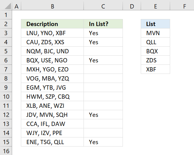
The image above shows an array formula in cell C3 that checks if cell B3 contains at least one of the values in List (E3:E7), it returns «Yes» if any of the values are found in column B and returns nothing if the cell contains none of the values.
For example, cell B3 contains XBF which is found in cell E7. Cell B4 contains text ZDS found in cell E6. Cell C5 contains no values in the list.
=IF(OR(COUNTIF(B3,»*»&$E$3:$E$7&»*»)), «Yes», «»)
You need to enter this formula as an array formula if you are not an Excel 365 subscriber. There is another formula below that doesn’t need to be entered as an array formula, however, it is slightly larger and more complicated.
- Type formula in cell C3.
- Press and hold CTRL + SHIFT simultaneously.
- Press Enter once.
- Release all keys.
Excel adds curly brackets to the formula automatically if you successfully entered the array formula. Don’t enter the curly brackets yourself.
Back to top
1.1 Explaining formula in cell C3
Step 1 — Check if the cell contains any of the values in the list
The COUNTIF function lets you count cells based on a condition, however, it also allows you to count cells based on multiple conditions if you use a cell range instead of a cell.
COUNTIF(range, criteria)
The criteria argument utilizes a beginning and ending asterisk in order to match a text string and not the entire cell value, asterisks are one of two wildcard characters that you are allowed to use.
The ampersands concatenate the asterisks to cell range E3:E7.
COUNTIF(B3,»*»&$E$3:$E$7&»*»)
becomes
COUNTIF(«LNU, YNO, XBF», {«*MVN*»; «*QLL*»; «*BQX*»; «*ZDS*»; «*XBF*»})
and returns this array
{0; 0; 0; 0; 1}
which tells us that the last value in the list is found in cell B3.
Step 2 — Return TRUE if at least one value is 1
The OR function returns TRUE if at least one of the values in the array is TRUE, the numerical equivalent to TRUE is 1.
OR({0; 0; 0; 0; 1})
returns TRUE.
Step 3 — Return Yes or nothing
The IF function then returns «Yes» if the logical test evaluates to TRUE and nothing if the logical test returns FALSE.
IF(TRUE, «Yes», «»)
returns «Yes» in cell B3.
Back to top
Regular formula
The following formula is quite similar to the formula above except that it is a regular formula and it has an additional INDEX function.
=IF(OR(INDEX(COUNTIF(B3,»*»&$E$3:$E$7&»*»),)), «Yes», «»)
Back to top
Back to top
2. Display matches if the cell contains text from a list

The image above demonstrates a formula that checks if a cell contains a value in the list and then returns that value. If multiple values match then all matching values in the list are displayed.
For example, cell B3 contains «ZDS, YNO, XBF» and cell range E3:E7 has two values that match, «ZDS» and «XBF».
Formula in cell C3:
=TEXTJOIN(«, «, TRUE, IF(COUNTIF(B3, «*»&$E$3:$E$7&»*»), $E$3:$E$7, «»))
The TEXTJOIN function is available for Office 2019 and Office 365 subscribers. You will get a #NAME error if your Excel version is missing this function. Office 2019 users may need to enter this formula as an array formula.
The next formula works with most Excel versions.
Array formula in cell C3:
=INDEX($E$3:$E$7, MATCH(1, COUNTIF(B3, «*»&$E$3:$E$7&»*»), 0))
However, it only returns the first match. There is another formula below that returns all matching values, check it out.
How to enter an array formula
Back to top
2.1 Explaining formula in cell C3
Step 1 — Count cells containing text strings
The COUNTIF function lets you count cells based on a condition, we are going to use multiple conditions. I am going to use asterisks to make the COUNTIF function check for a partial match.
The asterisk is one of two wild card characters that you can use, it matches 0 (zero) to any number of any characters.
COUNTIF(B3, «*»&$E$3:$E$7&»*»)
becomes
COUNTIF(«ZDS, YNO, XBF», {«*MVN*»; «*QLL*»; «*BQX*»; «*ZDS*»; «*XBF*»})
and returns {1; 0; 0; 0; 1}.
This array contains as many values as there values in the list, the position of each value in the array matches the position of the value in the list. This means that we can tell from the array that the first value and the last value is found in cell B3.
Step 2 — Return the actual value
The IF function returns one value if the logical test is TRUE and another value if the logical test is FALSE.
IF(logical_test, [value_if_true], [value_if_false])
This allows us to create an array containing values that exists in cell B3.
IF(COUNTIF(B3, «*»&$E$3:$E$7&»*»), $E$3:$E$7, «»)
becomes
IF(COUNTIF(«ZDS, YNO, XBF», {«*MVN*»; «*QLL*»; «*BQX*»; «*ZDS*»; «*XBF*»}), {«*MVN*»; «*QLL*»; «*BQX*»; «*ZDS*»; «*XBF*»}, «»)
and returns {«»;»»;»»;»ZDS»;»XBF»}.
Step 3 — Concatenate values in array
The TEXTJOIN function allows you to combine text strings from multiple cell ranges and also use delimiting characters if you want.
TEXTJOIN(delimiter, ignore_empty, text1, [text2], …)
TEXTJOIN(«, «, TRUE, IF(COUNTIF(B3, «*»&$E$3:$E$7&»*»), $E$3:$E$7, «»))
becomes
TEXTJOIN(«, «, TRUE, {«»;»»;»»;»ZDS»;»XBF»})
and returns text strings ZDS, XBF.
Back to top
3. Display matches if cell contains text from a list (Earlier Excel versions)

The image above demonstrates a formula that returns multiple matches if the cell contains values from a list. This array formula works with most Excel versions.
Array formula in cell C3:
=IFERROR(INDEX($G$3:$G$7, SMALL(IF(COUNTIF($B3, «*»&$G$3:$G$7&»*»), MATCH(ROW($G$3:$G$7), ROW($G$3:$G$7)), «»), COLUMNS($A$1:A1))), «»)
How to enter an array formula
Copy cell C3 and paste to cell range C3:E15.
Back to top
3.1 Explaining formula in cell C3
Step 1 — Identify matching values in cell
The COUNTIF function lets you count cells based on a condition, we are going to use a cell range instead. This will return an array of values.
COUNTIF($B3, «*»&$G$3:$G$7&»*»)
becomes
COUNTIF(«ZDS, YNO, XBF», {«*MVN*»; «*QLL*»; «*BQX*»; «*ZDS*»; «*XBF*»})
and returns {0; 0; 0; 1; 1}.
Step 2 — Calculate relative positions of matching values
The IF function returns one value if the logical test is TRUE and another value if the logical test is FALSE.
IF(logical_test, [value_if_true], [value_if_false])
This allows us to create an array containing values representing row numbers.
IF(COUNTIF($B3, «*»&$G$3:$G$7&»*»), MATCH(ROW($G$3:$G$7), ROW($G$3:$G$7)), «»)
becomes
IF({0; 0; 0; 2; 1}, MATCH(ROW($G$3:$G$7), ROW($G$3:$G$7)), «»)
becomes
IF({0; 0; 0; 2; 1}, {1; 2; 3; 4; 5}, «»)
and returns {«»; «»; «»; 4; 5}.
Step 3 — Extract the k-th smallest number
I am going to use the SMALL function to be able to extract one value in each cell in the next step.
SMALL(array, k)
SMALL(IF(COUNTIF($B3, «*»&$G$3:$G$7&»*»), MATCH(ROW($G$3:$G$7), ROW($G$3:$G$7)), «»), COLUMNS($A$1:A1)))
becomes
SMALL({«»; «»; «»; 4; 5}, COLUMNS($A$1:A1)))
The COLUMNS function calculates the number of columns in a cell range, however, the cell reference in our formula grows when you copy the cell and paste to adjacent cells to the right.
SMALL({0; 0; 0; 4; 5}, COLUMNS($A$1:A1)))
becomes
SMALL({«»; «»; «»; 4; 5}, 1)
and returns 4.
Step 4 — Return value based on row number
The INDEX function returns a value from a cell range or array, you specify which value based on a row and column number. Both the [row_num] and [column_num] are optional.
INDEX(array, [row_num], [column_num])
INDEX($G$3:$G$7, SMALL(IF(COUNTIF($B3, «*»&$G$3:$G$7&»*»), MATCH(ROW($G$3:$G$7), ROW($G$3:$G$7)), «»), COLUMNS($A$1:A1)))
becomes
INDEX($G$3:$G$7, 4)
becomes
INDEX({«MVN»;»QLL»;»BQX»;»ZDS»;»XBF»}, 4)
and returns «ZDS» in cell C3.
Step 5 — Remove error values
The IFERROR function lets you catch most errors in Excel formulas except #SPILL! errors. Be careful when using the IFERROR function, it may make it much harder spotting formula errors.
IFERROR(value, value_if_error)
There are two arguments in the IFERROR function. The value argument is returned if it is not evaluating to an error. The value_if_error argument is returned if the value argument returns an error.
IFERROR(INDEX($G$3:$G$7, SMALL(IF(COUNTIF($B3, «*»&$G$3:$G$7&»*»), MATCH(ROW($G$3:$G$7), ROW($G$3:$G$7)), «»), COLUMNS($A$1:A1))), «»)
Back to top
4. Filter delimited values not in the list (Excel 365)

The formula in cell C3 lists values in cell B3 that are not in the List specified in cell range E3:E7. The formula returns #CALC! error if all values are in the list, see cell C14 as an example.
Excel 365 dynamic array formula in cell C3:
=LET(z,TRIM(TEXTSPLIT(B3,,»,»)),TEXTJOIN(«, «,TRUE,FILTER(z,NOT(COUNTIF($E$3:$E$7,z)))))
4.1 Explaining formula
Step 1 — Split values with a delimiting character
The TEXTSPLIT function splits a string into an array based on delimiting values.
Function syntax: TEXTSPLIT(Input_Text, col_delimiter, [row_delimiter], [Ignore_Empty])
TEXTSPLIT(B3,,»,»)
becomes
TEXTSPLIT(«ZDS, VTO, XBF»,,»,»)
and returns
{«ZDS»; » VTO»; » XBF»}
Step 2 — Remove leading and trailing spaces
The TRIM function deletes all blanks or space characters except single blanks between words in a cell value.
Function syntax: TRIM(text)
TRIM(TEXTSPLIT(B3,,»,»))
becomes
TRIM({«ZDS»; » VTO»; » XBF»})
and returns
{«ZDS»; «VTO»; «XBF»}
Step 3 — Check if values are in list
The COUNTIF function calculates the number of cells that is equal to a condition.
Function syntax: COUNTIF(range, criteria)
COUNTIF($E$3:$E$7,TRIM(TEXTSPLIT(B3,,»,»)))
becomes
COUNTIF({«MVN»;»QLL»;»BQX»;»ZDS»;»XBF»},{«ZDS»; «VTO»; «XBF»})
and returns
{1; 0; 1}
These numbers indicate if a value is found in the list, zero means not in the list and 1 or higher means that the value is in the list at least once.
The number’s position corresponds to the position of the values. {1; 0; 1} — {«ZDS»; «VTO»; «XBF»} meaning «ZDS» and «XBF» are in the list and «VTO» not.
Step 4 — Not
The NOT function returns the boolean opposite to the given argument.
Function syntax: NOT(logical)
NOT(COUNTIF($E$3:$E$7,TRIM(TEXTSPLIT(B3,,»,»))))
becomes
NOT({1; 0; 1})
and returns
{FALSE; TRUE; FALSE}.
0 (zero) is equivalent to FALSE. The boolean opposite is TRUE.
Any other number than 0 (zero) is equivalent to TRUE. The boolean opposite is FALSE.
Step 5 — Filter
The FILTER function extracts values/rows based on a condition or criteria.
Function syntax: FILTER(array, include, [if_empty])
FILTER(TRIM(TEXTSPLIT(B3,,»,»)),NOT(COUNTIF($E$3:$E$7,TRIM(TEXTSPLIT(B3,,»,»)))))
becomes
FILTER({«ZDS»; «VTO»; «XBF»},{FALSE; TRUE; FALSE})
and returns
«VTO».
Step 6 — Join
The TEXTJOIN function combines text strings from multiple cell ranges.
Function syntax: TEXTJOIN(delimiter, ignore_empty, text1, [text2], …)
TEXTJOIN(«, «,TRUE,FILTER(TRIM(TEXTSPLIT(B3,,»,»)),NOT(COUNTIF($E$3:$E$7,TRIM(TEXTSPLIT(B3,,»,»))))))
becomes
TEXTJOIN(«, «,TRUE,{«VTO»})
and returns
«VTO».
Step 7 — Shorten the formula
The LET function lets you name intermediate calculation results which can shorten formulas considerably and improve performance.
Function syntax: LET(name1, name_value1, calculation_or_name2, [name_value2, calculation_or_name3…])
TEXTJOIN(«, «,TRUE,FILTER(TRIM(TEXTSPLIT(B3,,»,»)),NOT(COUNTIF($E$3:$E$7,TRIM(TEXTSPLIT(B3,,»,»))))))
z — TRIM(TEXTSPLIT(B3,,»,»))
LET(z,TRIM(TEXTSPLIT(B3,,»,»)),TEXTJOIN(«, «,TRUE,FILTER(z,NOT(COUNTIF($E$3:$E$7,z)))))
Back to top