Excel if any of these values

Excel has a number of formulas that help you use your data in useful ways. For example, you can get an output based on whether or not a cell meets certain specifications. Right now, we’ll focus on a function called “if cell contains, then”. Let’s look at an example.

Jump To Specific Section:

1. Explanation: If Cell Contains
2. If cell contains any value, then return a value
3. If cell contains text/number, then return a value
4. If cell contains specific text, then return a value
5. If cell contains specific text, then return a value (case-sensitive)
6. If cell does not contain specific text, then return a value
7. If cell contains one of many text strings, then return a value
8. If cell contains several of many text strings, then return a value

Excel Formula: If cell contains

Generic formula 

=IF(ISNUMBER(SEARCH("abc",A1)),A1,"")

=IF(ISNUMBER(SEARCH("abc",B5)),B5,"")

If you want to check whether or not the A1 cell contains the text “Example”, you can run a formula that will output “Yes” or “No” in the B1 cell. There are a number of different ways you can put these formulas to use. At the time of writing, Excel is able to return the following variations:

• If cell contains any value
  
• If cell contains text
• If cell contains number
• If cell contains specific text
• If cell contains certain text string
• If cell contains one of many text strings
• If cell contains several strings

Using these scenarios, you’re able to check if a cell contains text, value, and more. 

Explanation: If Cell Contains

=IF(ISNUMBER(SEARCH("abc",B5)),B5,""). Assuming cells run to B5

ISNUMBER(SEARCH("abc",B5))

Read article: Excel efficiency: 11 Excel Formulas To Increase Your Productivity

Using “if cell contains” formulas in Excel

The guides below were written using the latest Microsoft Excel 2019 for Windows 10. Some steps may vary if you’re using a different version or platform. Contact our experts if you need any further assistance.

1. If cell contains any value, then return a value

This scenario allows you to return values based on whether or not a cell contains any value at all. For example, we’ll be checking whether or not the A1 cell is blank or not, and then return a value depending on the result.

• Select the output cell, and use the following formula: =IF(cell<>»», value_to_return, «»).
• For our example, the cell we want to check is A2, and the return value will be No. In this scenario, you’d change the formula to =IF(A2<>»», «No», «»). 
• Since the A2 cell isn’t blank, the formula will return “No” in the output cell. If the cell you’re checking is blank, the output cell will also remain blank.

2. If cell contains text/number, then return a value

With the formula below, you can return a specific value if the target cell contains any text or number. The formula will ignore the opposite data types.

Check for text

• To check if a cell contains text, select the output cell, and use the following formula: =IF(ISTEXT(cell), value_to_return, «»).
• For our example, the cell we want to check is A2, and the return value will be Yes. In this scenario, you’d change the formula to =IF(ISTEXT(A2), «Yes», «»). 
  
  
• Because the A2 cell does contain text and not a number or date, the formula will return “Yes” into the output cell.

Check for a number or date

• To check if a cell contains a number or date, select the output cell, and use the following formula: =IF(ISNUMBER(cell), value_to_return, «»).
• For our example, the cell we want to check is D2, and the return value will be Yes. In this scenario, you’d change the formula to =IF(ISNUMBER(D2), «Yes», «»). 
  
  
• Because the D2 cell does contain a number and not text, the formula will return “Yes” into the output cell.

3. If cell contains specific text, then return a value

To find a cell that contains specific text, use the formula below.

• Select the output cell, and use the following formula: =IF(cell=»text», value_to_return, «»).
• For our example, the cell we want to check is A2, the text we’re looking for is “example”, and the return value will be Yes. In this scenario, you’d change the formula to =IF(A2=»example», «Yes», «»). 
  
  
• Because the A2 cell does consist of the text “example”, the formula will return “Yes” into the output cell.

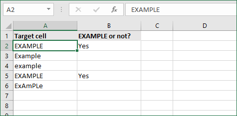
4. If cell contains specific text, then return a value (case-sensitive)

To find a cell that contains specific text, use the formula below. This version is case-sensitive, meaning that only cells with an exact match will return the specified value.

• Select the output cell, and use the following formula: =IF(EXACT(cell,»case_sensitive_text»), «value_to_return», «»).
• For our example, the cell we want to check is A2, the text we’re looking for is “EXAMPLE”, and the return value will be Yes. In this scenario, you’d change the formula to =IF(EXACT(A2,»EXAMPLE»), «Yes», «»).
• Because the A2 cell does consist of the text “EXAMPLE” with the matching case, the formula will return “Yes” into the output cell.

5. If cell does not contain specific text, then return a value

The opposite version of the previous section. If you want to find cells that don’t contain a specific text, use this formula.

• Select the output cell, and use the following formula: =IF(cell=»text», «», «value_to_return»).
• For our example, the cell we want to check is A2, the text we’re looking for is “example”, and the return value will be No. In this scenario, you’d change the formula to =IF(A2=»example», «», «No»).
  
• Because the A2 cell does consist of the text “example”, the formula will return a blank cell. On the other hand, other cells return “No” into the output cell.

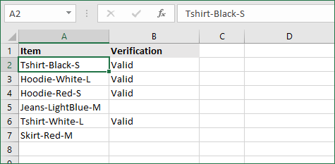
6. If cell contains one of many text strings, then return a value

This formula should be used if you’re looking to identify cells that contain at least one of many words you’re searching for.

• Select the output cell, and use the following formula: =IF(OR(ISNUMBER(SEARCH(«string1», cell)), ISNUMBER(SEARCH(«string2», cell))), value_to_return, «»).
• For our example, the cell we want to check is A2. We’re looking for either “tshirt” or “hoodie”, and the return value will be Valid. In this scenario, you’d change the formula to =IF(OR(ISNUMBER(SEARCH(«tshirt»,A2)),ISNUMBER(SEARCH(«hoodie»,A2))),»Valid «,»»).
  
  
• Because the A2 cell does contain one of the text values we searched for, the formula will return “Valid” into the output cell.

To extend the formula to more search terms, simply modify it by adding more strings using ISNUMBER(SEARCH(«string», cell)).

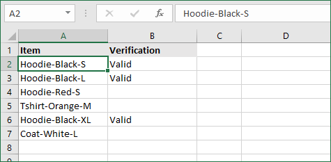
7. If cell contains several of many text strings, then return a value

This formula should be used if you’re looking to identify cells that contain several of the many words you’re searching for. For example, if you’re searching for two terms, the cell needs to contain both of them in order to be validated.

• Select the output cell, and use the following formula: =IF(AND(ISNUMBER(SEARCH(«string1»,cell)), ISNUMBER(SEARCH(«string2″,cell))), value_to_return,»»).
• For our example, the cell we want to check is A2. We’re looking for “hoodie” and “black”, and the return value will be Valid. In this scenario, you’d change the formula to =IF(AND(ISNUMBER(SEARCH(«hoodie»,A2)),ISNUMBER(SEARCH(«black»,A2))),»Valid «,»»).
  
  
• Because the A2 cell does contain both of the text values we searched for, the formula will return “Valid” to the output cell.

Final thoughts

We hope this article was useful to you in learning how to use “if cell contains” formulas in Microsoft Excel. Now, you can check if any cells contain values, text, numbers, and more. This allows you to navigate, manipulate and analyze your data efficiently.

We’re glad you’re read the article up to here Thank you

You may also like

» How to use NPER Function in Excel
» How to Separate First and Last Name in Excel
» How to Calculate Break-Even Analysis in Excel

Author: Oscar Cronquist Article last updated on February 01, 2023

This article demonstrates several ways to check if a cell contains any value based on a list. The first example shows how to check if any of the values in the list is in the cell.

The remaining examples show formulas that also return the matching values. You may need different formulas based on the Excel version you are using.

Read this article If cell equals value from list to match the entire cell to any value from a list. To match a single cell to a single value read this: If cell contains text

To check if a cell contains all values in the list read this: If cell contains multiple values

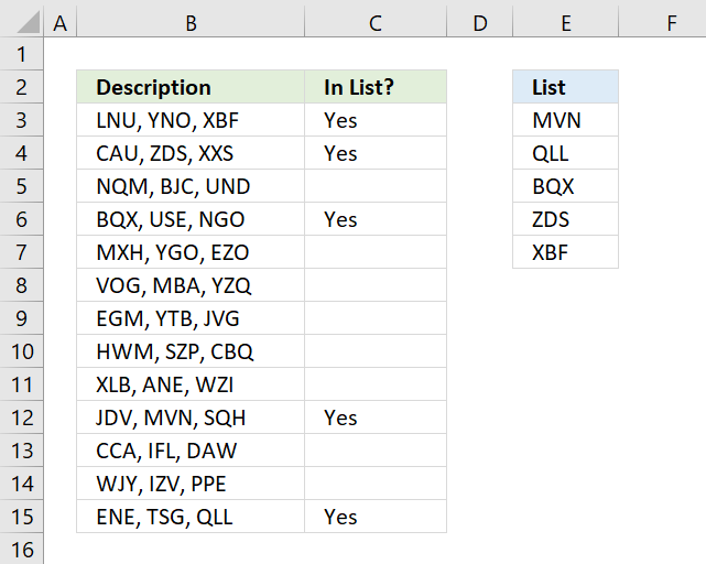
1. Check if the cell contains any value in the list

The image above shows an array formula in cell C3 that checks if cell B3 contains at least one of the values in List (E3:E7), it returns «Yes» if any of the values are found in column B and returns nothing if the cell contains none of the values.

For example, cell B3 contains XBF which is found in cell E7. Cell B4 contains text ZDS found in cell E6. Cell C5 contains no values in the list.

=IF(OR(COUNTIF(B3,»*»&$E$3:$E$7&»*»)), «Yes», «»)

You need to enter this formula as an array formula if you are not an Excel 365 subscriber. There is another formula below that doesn’t need to be entered as an array formula, however, it is slightly larger and more complicated.

1. Type formula in cell C3.
2. Press and hold CTRL + SHIFT simultaneously.
3.  Press Enter once.
4. Release all keys.

Excel adds curly brackets to the formula automatically if you successfully entered the array formula. Don’t enter the curly brackets yourself.

Back to top

1.1 Explaining formula in cell C3

Step 1 — Check if the cell contains any of the values in the list

The COUNTIF function lets you count cells based on a condition, however, it also allows you to count cells based on multiple conditions if you use a cell range instead of a cell.

COUNTIF(range, criteria)

The criteria argument utilizes a beginning and ending asterisk in order to match a text string and not the entire cell value, asterisks are one of two wildcard characters that you are allowed to use.

The ampersands concatenate the asterisks to cell range E3:E7.

COUNTIF(B3,»*»&$E$3:$E$7&»*»)

becomes

COUNTIF(«LNU, YNO, XBF», {«*MVN*»; «*QLL*»; «*BQX*»; «*ZDS*»; «*XBF*»})

and returns this array

{0; 0; 0; 0; 1}

which tells us that the last value in the list is found in cell B3.

Step 2 — Return TRUE if at least one value is 1

The OR function returns TRUE if at least one of the values in the array is TRUE, the numerical equivalent to TRUE is 1.

OR({0; 0; 0; 0; 1})

returns TRUE.

Step 3 — Return Yes or nothing

The IF function then returns «Yes» if the logical test evaluates to TRUE and nothing if the logical test returns FALSE.

IF(TRUE, «Yes», «»)

returns «Yes» in cell B3.

Back to top

Regular formula

The following formula is quite similar to the formula above except that it is a regular formula and it has an additional INDEX function.

=IF(OR(INDEX(COUNTIF(B3,»*»&$E$3:$E$7&»*»),)), «Yes», «»)

Back to top

Back to top

2. Display matches if the cell contains text from a list

The image above demonstrates a formula that checks if a cell contains a value in the list and then returns that value. If multiple values match then all matching values in the list are displayed.

For example, cell B3 contains «ZDS, YNO, XBF» and cell range E3:E7 has two values that match, «ZDS» and «XBF».

Formula in cell C3:

=TEXTJOIN(«, «, TRUE, IF(COUNTIF(B3, «*»&$E$3:$E$7&»*»), $E$3:$E$7, «»))

The TEXTJOIN function is available for Office 2019 and Office 365 subscribers. You will get a #NAME error if your Excel version is missing this function. Office 2019 users may need to enter this formula as an array formula.

The next formula works with most Excel versions.

Array formula in cell C3:

=INDEX($E$3:$E$7, MATCH(1, COUNTIF(B3, «*»&$E$3:$E$7&»*»), 0))

However, it only returns the first match. There is another formula below that returns all matching values, check it out.

How to enter an array formula

Back to top

2.1 Explaining formula in cell C3

Step 1 — Count cells containing text strings

The COUNTIF function lets you count cells based on a condition, we are going to use multiple conditions. I am going to use asterisks to make the COUNTIF function check for a partial match.

The asterisk is one of two wild card characters that you can use, it matches 0 (zero) to any number of any characters.

COUNTIF(B3, «*»&$E$3:$E$7&»*»)

becomes

COUNTIF(«ZDS, YNO, XBF», {«*MVN*»; «*QLL*»; «*BQX*»; «*ZDS*»; «*XBF*»})

and returns {1; 0; 0; 0; 1}.

This array contains as many values as there values in the list, the position of each value in the array matches the position of the value in the list. This means that we can tell from the array that the first value and the last value is found in cell B3.

Step 2 — Return the actual value

The IF function returns one value if the logical test is TRUE and another value if the logical test is FALSE.

IF(logical_test, [value_if_true], [value_if_false])

This allows us to create an array containing values that exists in cell B3.

IF(COUNTIF(B3, «*»&$E$3:$E$7&»*»), $E$3:$E$7, «»)

becomes

IF(COUNTIF(«ZDS, YNO, XBF», {«*MVN*»; «*QLL*»; «*BQX*»; «*ZDS*»; «*XBF*»}), {«*MVN*»; «*QLL*»; «*BQX*»; «*ZDS*»; «*XBF*»}, «»)

and returns {«»;»»;»»;»ZDS»;»XBF»}.

Step 3 — Concatenate values in array

The TEXTJOIN function allows you to combine text strings from multiple cell ranges and also use delimiting characters if you want.

TEXTJOIN(delimiter, ignore_empty, text1, [text2], …)

TEXTJOIN(«, «, TRUE, IF(COUNTIF(B3, «*»&$E$3:$E$7&»*»), $E$3:$E$7, «»))

becomes

TEXTJOIN(«, «, TRUE, {«»;»»;»»;»ZDS»;»XBF»})

and returns text strings ZDS, XBF.

Back to top

3. Display matches if cell contains text from a list (Earlier Excel versions)

The image above demonstrates a formula that returns multiple matches if the cell contains values from a list. This array formula works with most Excel versions.

Array formula in cell C3:

=IFERROR(INDEX($G$3:$G$7, SMALL(IF(COUNTIF($B3, «*»&$G$3:$G$7&»*»), MATCH(ROW($G$3:$G$7), ROW($G$3:$G$7)), «»), COLUMNS($A$1:A1))), «»)

How to enter an array formula

Copy cell C3 and paste to cell range C3:E15.

Back to top

3.1 Explaining formula in cell C3

Step 1 — Identify matching values in cell

The COUNTIF function lets you count cells based on a condition, we are going to use a cell range instead. This will return an array of values.

COUNTIF($B3, «*»&$G$3:$G$7&»*»)

becomes

COUNTIF(«ZDS, YNO, XBF», {«*MVN*»; «*QLL*»; «*BQX*»; «*ZDS*»; «*XBF*»})

and returns {0; 0; 0; 1; 1}.

Step 2 — Calculate relative positions of matching values

The IF function returns one value if the logical test is TRUE and another value if the logical test is FALSE.

IF(logical_test, [value_if_true], [value_if_false])

This allows us to create an array containing values representing row numbers.

IF(COUNTIF($B3, «*»&$G$3:$G$7&»*»), MATCH(ROW($G$3:$G$7), ROW($G$3:$G$7)), «»)

becomes

IF({0; 0; 0; 2; 1}, MATCH(ROW($G$3:$G$7), ROW($G$3:$G$7)), «»)

becomes

IF({0; 0; 0; 2; 1}, {1; 2; 3; 4; 5}, «»)

and returns {«»; «»; «»; 4; 5}.

Step 3 — Extract the k-th smallest number

I am going to use the SMALL function to be able to extract one value in each cell in the next step.

SMALL(array, k)

SMALL(IF(COUNTIF($B3, «*»&$G$3:$G$7&»*»), MATCH(ROW($G$3:$G$7), ROW($G$3:$G$7)), «»), COLUMNS($A$1:A1)))

becomes

SMALL({«»; «»; «»; 4; 5}, COLUMNS($A$1:A1)))

The COLUMNS function calculates the number of columns in a cell range, however, the cell reference in our formula grows when you copy the cell and paste to adjacent cells to the right.

SMALL({0; 0; 0; 4; 5}, COLUMNS($A$1:A1)))

becomes

SMALL({«»; «»; «»; 4; 5}, 1)

and returns 4.

Step 4 — Return value based on row number

The INDEX function returns a value from a cell range or array, you specify which value based on a row and column number. Both the [row_num] and [column_num] are optional.

INDEX(array, [row_num], [column_num])

INDEX($G$3:$G$7, SMALL(IF(COUNTIF($B3, «*»&$G$3:$G$7&»*»), MATCH(ROW($G$3:$G$7), ROW($G$3:$G$7)), «»), COLUMNS($A$1:A1)))

becomes

INDEX($G$3:$G$7, 4)

becomes

INDEX({«MVN»;»QLL»;»BQX»;»ZDS»;»XBF»}, 4)

and returns «ZDS» in cell C3.

Step 5 — Remove error values

The IFERROR function lets you catch most errors in Excel formulas except #SPILL! errors. Be careful when using the IFERROR function, it may make it much harder spotting formula errors.

IFERROR(value, value_if_error)

There are two arguments in the IFERROR function. The value argument is returned if it is not evaluating to an error. The value_if_error argument is returned if the value argument returns an error.

IFERROR(INDEX($G$3:$G$7, SMALL(IF(COUNTIF($B3, «*»&$G$3:$G$7&»*»), MATCH(ROW($G$3:$G$7), ROW($G$3:$G$7)), «»), COLUMNS($A$1:A1))), «»)

Back to top

4. Filter delimited values not in the list (Excel 365)

The formula in cell C3 lists values in cell B3 that are not in the List specified in cell range E3:E7. The formula returns #CALC! error if all values are in the list, see cell C14 as an example.

Excel 365 dynamic array formula in cell C3:

=LET(z,TRIM(TEXTSPLIT(B3,,»,»)),TEXTJOIN(«, «,TRUE,FILTER(z,NOT(COUNTIF($E$3:$E$7,z)))))

4.1 Explaining formula

Step 1 — Split values with a delimiting character

The TEXTSPLIT function splits a string into an array based on delimiting values.

Function syntax: TEXTSPLIT(Input_Text, col_delimiter, [row_delimiter], [Ignore_Empty])

TEXTSPLIT(B3,,»,»)

becomes

TEXTSPLIT(«ZDS, VTO, XBF»,,»,»)

and returns

{«ZDS»; » VTO»; » XBF»}

Step 2 — Remove leading and trailing spaces

The TRIM function deletes all blanks or space characters except single blanks between words in a cell value.

Function syntax: TRIM(text)

TRIM(TEXTSPLIT(B3,,»,»))

becomes

TRIM({«ZDS»; » VTO»; » XBF»})

and returns

{«ZDS»; «VTO»; «XBF»}

Step 3 — Check if values are in list

The COUNTIF function calculates the number of cells that is equal to a condition.

Function syntax: COUNTIF(range, criteria)

COUNTIF($E$3:$E$7,TRIM(TEXTSPLIT(B3,,»,»)))

becomes

COUNTIF({«MVN»;»QLL»;»BQX»;»ZDS»;»XBF»},{«ZDS»; «VTO»; «XBF»})

and returns

{1; 0; 1}

These numbers indicate if a value is found in the list, zero means not in the list and 1 or higher means that the value is in the list at least once.

The number’s position corresponds to the position of the values. {1; 0; 1} — {«ZDS»; «VTO»; «XBF»} meaning «ZDS» and «XBF» are in the list and «VTO» not.

Step 4 — Not

The NOT function returns the boolean opposite to the given argument.

Function syntax: NOT(logical)

NOT(COUNTIF($E$3:$E$7,TRIM(TEXTSPLIT(B3,,»,»))))

becomes

NOT({1; 0; 1})

and returns

{FALSE; TRUE; FALSE}.

0 (zero) is equivalent to FALSE. The boolean opposite is TRUE.

Any other number than 0 (zero) is equivalent to TRUE.  The boolean opposite is FALSE.

Step 5 — Filter

The FILTER function extracts values/rows based on a condition or criteria.

Function syntax: FILTER(array, include, [if_empty])

FILTER(TRIM(TEXTSPLIT(B3,,»,»)),NOT(COUNTIF($E$3:$E$7,TRIM(TEXTSPLIT(B3,,»,»)))))

becomes

FILTER({«ZDS»; «VTO»; «XBF»},{FALSE; TRUE; FALSE})

and returns

«VTO».

Step 6 — Join

The TEXTJOIN function combines text strings from multiple cell ranges.

Function syntax: TEXTJOIN(delimiter, ignore_empty, text1, [text2], …)

TEXTJOIN(«, «,TRUE,FILTER(TRIM(TEXTSPLIT(B3,,»,»)),NOT(COUNTIF($E$3:$E$7,TRIM(TEXTSPLIT(B3,,»,»))))))

becomes

TEXTJOIN(«, «,TRUE,{«VTO»})

and returns

«VTO».

Step 7 — Shorten the formula

The LET function lets you name intermediate calculation results which can shorten formulas considerably and improve performance.

Function syntax: LET(name1, name_value1, calculation_or_name2, [name_value2, calculation_or_name3…])

TEXTJOIN(«, «,TRUE,FILTER(TRIM(TEXTSPLIT(B3,,»,»)),NOT(COUNTIF($E$3:$E$7,TRIM(TEXTSPLIT(B3,,»,»))))))

z — TRIM(TEXTSPLIT(B3,,»,»))

LET(z,TRIM(TEXTSPLIT(B3,,»,»)),TEXTJOIN(«, «,TRUE,FILTER(z,NOT(COUNTIF($E$3:$E$7,z)))))

Back to top

To perform complicated and powerful data analysis, you need to test various conditions at a single point in time. The data analysis might require logical tests also within these multiple conditions.

For this, you need to perform Excel if statement with multiple conditions or ranges that include various If functions in a single formula.

Those who use Excel daily are well versed with Excel If statement as it is one of the most-used formula. Here you can check various Excel If or statement, Nested If, AND function, Excel IF statements, and how to use them. We have also provided a VIDEO TUTORIAL for different If Statements.

There are various If statements available in Excel. You have to know which of the Excel If you will work at what condition. Here you can check multiple conditions where you can use Excel If statement.

1) Excel If Statement

If you want to test a condition to get two outcomes then you can use this Excel If statement.

=If(Marks>=40, “Pass”)

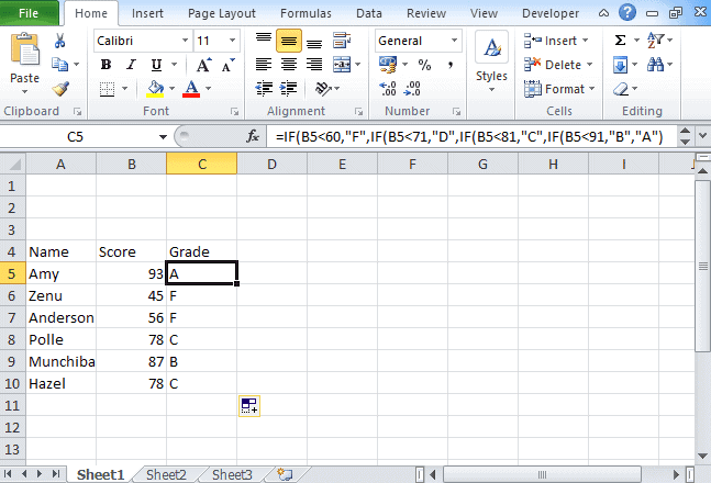
2) Nested If Statement

Let’s take an example that met the below-mentioned condition

• If the score is between 0 to 60, then Grade F
• If the score is between 61 to 70, then Grade D
• If the score is between 71 to 80, then Grade C
• If the score is between 81 to 90, then Grade B
• If the score is between 91 to 100, then Grade A

Then to test the condition the syntax of the formula becomes,

=If(B5<60, “F”,If(B5<71, “D”, If(B5<81,”C”,If(B5<91,”B”,”A”)

3) Excel If with Logical Test

There are 2 different types of conditions AND and OR. You can use the IF statement in excel between two values in both these conditions to perform the logical test.

AND Function: If you are performing the logical test based on AND function, then excel will give you TRUE as an outcome in every condition else it will return false.

OR Function: If you are using OR condition for the logical test, then excel will give you an outcome as TRUE if any of the situations match else it returns false.

For this, multiple testing is to be done using AND and OR function, you should gain expertise in using either or both of these with IF statement. Here we have used if the function with 3 conditions.

How to apply IF & AND function in Excel

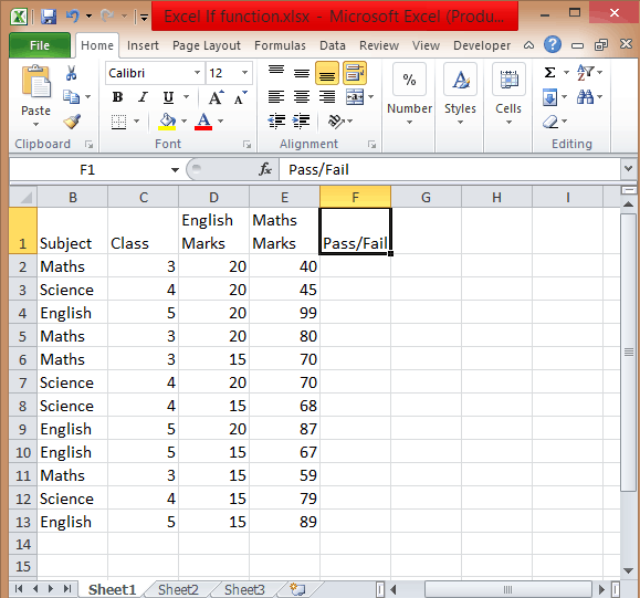
• To perform this multiple if and statements in excel, we will take the data set for the student’s marks that contain fields such as English and Math’s Marks.
• The score of the English subject is stored in the D column whereas the Maths score is stored in column E.
• Let say a student passes the class if his or her score in English is greater than or equal to 20 and he or she scores more than 60 in Maths.
• To create a report in matters of seconds, if formula combined with AND can suffice.
• Type =IF( Excel will display the logical hint just below the cell F2. The parameters of this function are logical_test, value_if_true, value_if_false.
• The first parameter contains the condition to be matched. You can use multiple If and AND conditions combined in this logical test.
• In the second parameter, type the value that you want Excel to display if the condition is true. Similarly, in the third parameter type the value that will be displayed if your condition is false.

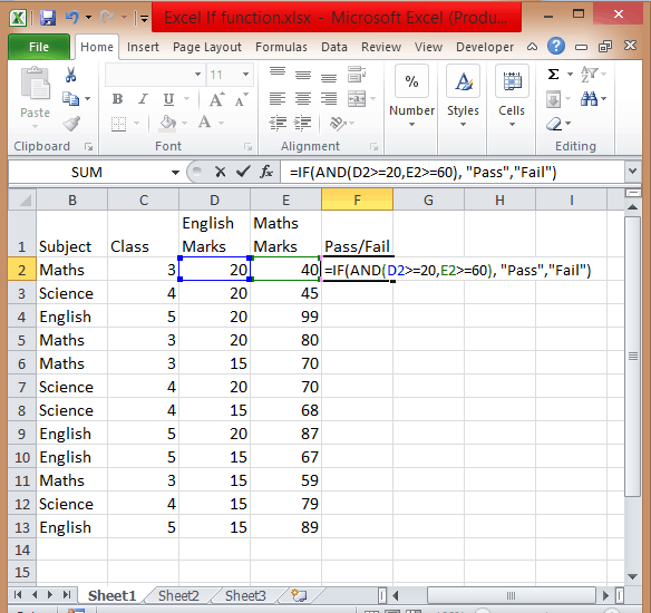
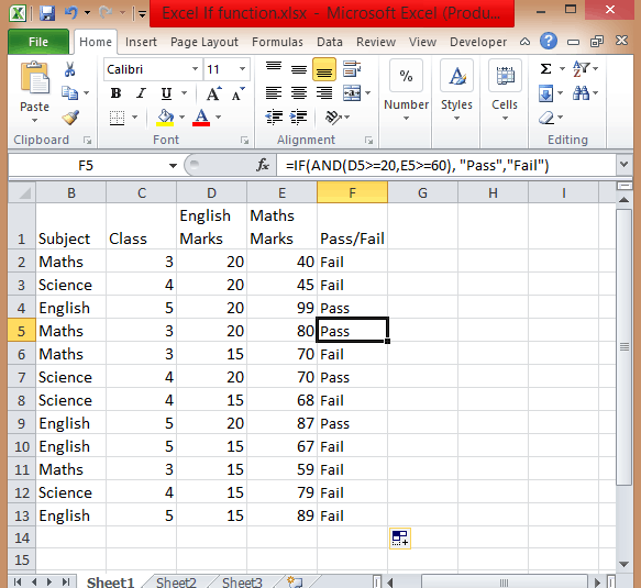
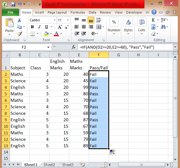
• Apply If & And formula, you will get =IF(AND(D2>=20,E2>=60),”Pass”,”Fail”).

• Add Pass/Fail column in the current table.

• After you have applied this formula, you will find the result in the column.
• Copy the formula from cell F2 and paste in all other cells from F3 to F13.

How to use If with Or function in Excel

To use If and Or statement excel, you need to apply a similar formula as you have applied for If & And with the only difference is that if any of the condition is true then it will show you True.

To apply the formula, you have to follow the above process. The formula is =IF((OR(D2>=20, E2>=60)), “Pass”, “Fail”). If the score is equal or greater than 20 for column D or the second score is equal or greater than 60 then the person is the pass.

How to Use If with And & Or function

If you want to test data based on several multiple conditions then you have to apply both And & Or functions at a single point in time. For example,

Situation 1: If column D>=20 and column E>=60

Situation 2: If column D>=15 and column E>=60

If any of the situations met, then the candidate is passed, else failed. The formula is

=IF(OR(AND(D2>=20, E2>=60), AND(D2>=20, E2>=60)), “Pass”, “Fail”).

4) Excel If Statement with other functions

Above we have learned how to use excel if statement multiple conditions range with And/Or functions. Now we will be going to learn Excel If Statement with other excel functions.

• Excel If with Sum, Average, Min, and Max functions

Let’s take an example where we want to calculate the performance of any student with Poor, Satisfactory, and Good.

If the data set has a predefined structure that will not allow any of the modifications. Then you can add values with this If formula:

=If((A2+B2)>=50, “Good”, If((A2+B2)=>30, “Satisfactory”, “Poor”))

Using the Sum function,

=If(Sum(A2:B2)>=120, “Good”, If(Sum(A2:B2)>=100, “Satisfactory”, “Poor”))

Using the Average function,

=If(Average(A2:B2)>=40, “Good”, If(Average(A2:B2)>=25, “Satisfactory”, “Poor”))

Using Max/Min,

If you want to find out the highest scores, using the Max function. You can also find the lowest scores using the Min function.

=If(C2=Max($C$2:$C$10), “Best result”, “ “)

You can also find the lowest scores using the Min function.

=If(C2=Min($C$2:$C$10), “Worst result”, “ “)

If we combine both these formulas together, then we get

=If(C2=Max($C$2:$C$10), “Best result”, If(C2=Min($C$2:$C$10), “Worst result”, “ “))

You can also call it as nested if functions with other excel functions. To get a result, you can use these if functions with various different functions that are used in excel.

So there are four different ways and types of excel if statements, that you can use according to the situation or condition. Start using it today.

So this is all about Excel If statement multiple conditions ranges, you can also check how to add bullets in excel in our next post.

I hope you found this tutorial useful

You may also like the following Excel tutorials:

• Multiple If Statements in Excel
• Excel Logical test
• How to Compare Two Columns in Excel (using VLOOKUP & IF)
• Using IF Function with Dates in Excel (Easy Examples)