Excel формулы if sum

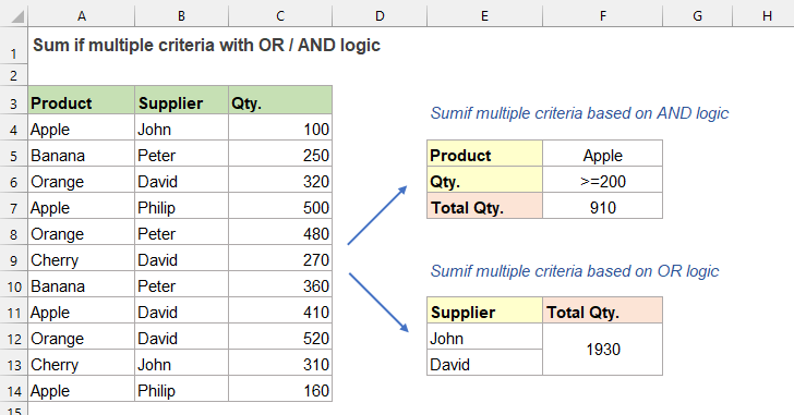
При работе с листами Excel вам может потребоваться суммировать значения на основе нескольких критериев. Иногда несколько критериев взяты из одного столбца (логика ИЛИ), но иногда из разных столбцов (логика И). В таком случае, как бы вы могли справиться с этой задачей в Excel?

• Sumif с несколькими критериями на основе логики ИЛИ
  • Используя формулу СУММЕСЛИ + СУММЕСЛИ +…
  • Используя функции СУММ и СУММЕСЛИ
• Sumif с несколькими критериями на основе логики И с использованием функции СУММЕСЛИМН

---

Sumif с несколькими критериями на основе логики ИЛИ

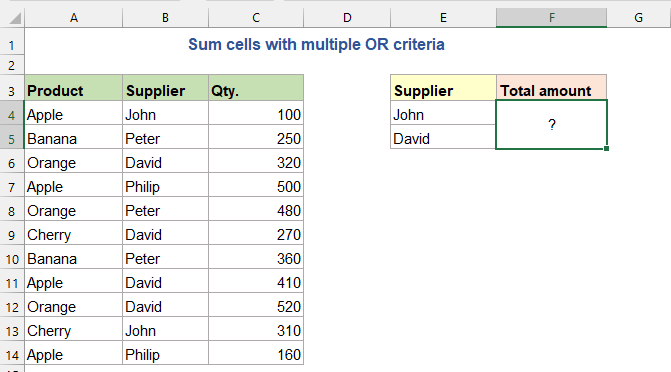
Предположим, у вас есть список продуктов, который содержит поставщика и количество, как показано на скриншоте ниже, теперь вы хотите получить все общие количества, которые поставляются поставщиком Джоном и Дэвидом. Здесь я представлю вам две простые формулы.

Используя формулу СУММЕСЛИ + СУММЕСЛИ +…

Если вы хотите суммировать числа, которые соответствуют любому из критериев (логика ИЛИ) из нескольких критериев, вы можете сложить несколько функций СУММЕСЛИ в одной формуле, общий синтаксис следующий:

=SUMIF(criteria_range, criteria1, sum_range)+SUMIF(criteria_range, criteria2, sum_range)+…

• criteria_range: Диапазон ячеек, который должен соответствовать критериям;
• criteria1: Первый критерий, используемый для определения суммирования ячеек;
• criteria2: Второй критерий, используемый для определения суммирования ячеек;
• sum_range: Диапазон ячеек, по которым вы хотите произвести суммирование.

Теперь скопируйте или введите любую из приведенных ниже формул в пустую ячейку и нажмите Enter ключ для получения результата:

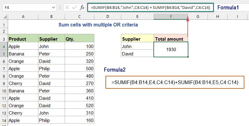
=SUMIF(B4:B14,«John»,C4:C14) + SUMIF(B4:B14,«David»,C4:C14)           (Type the criteria manually)
=SUMIF(B4:B14,E4,C4:C14) + SUMIF(B4:B14,E5,C4:C14)                           (Use a cell reference)

---

Пояснение к формуле:

=SUMIF(B4:B14,»John»,C4:C14) + SUMIF(B4:B14,»David»,C4:C14)

• Первый СУММЕСЛИ (B4: B14; «Джон»; C4: C14) находит строки Джона и суммирует общие количества;
• Второй СУММЕСЛИ (B4: B14, «Давид», C4: C14) находит строки Давида и суммирует общие количества;
• Затем сложите эти две формулы СУММЕСЛИ, чтобы получить все общие количества, предоставленные Джоном и Дэвидом.

---

Используя функции СУММ и СУММЕСЛИ

Приведенная выше формула очень проста в использовании, если есть только пара критериев, но если вы хотите суммировать значения с несколькими условиями ИЛИ, приведенная выше формула может быть избыточной. В этом случае лучшая формула, созданная на основе функций СУММ и СУММЕСЛИ, может оказать вам услугу. Общие синтаксисы:

Общая формула с жестко закодированным текстом:

=SUM(SUMIF(criteria_range, {criteria1,criteria2,…}, sum_range))

• criteria_range: Диапазон ячеек, который должен соответствовать критериям;
• criteria1: Первый критерий, используемый для определения суммирования ячеек;
• criteria2: Второй критерий, используемый для определения суммирования ячеек;
• sum_range: Диапазон ячеек, по которым вы хотите произвести суммирование.

Общая формула со ссылками на ячейки:

{=SUM(SUMIF(criteria_range, criteria_cells, sum_range))}
Array formula, should press Ctrl + Shift + Enter keys together.

• criteria_range: Диапазон ячеек, который должен соответствовать критериям;
• criteria_cells: Ячейки, содержащие критерии, которые вы хотите использовать;
• sum_range: Диапазон ячеек, по которым вы хотите произвести суммирование.

Пожалуйста, введите или скопируйте любую из приведенных ниже формул в пустую ячейку и получите результат:

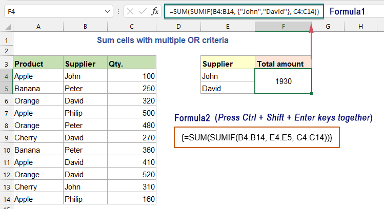
=SUM(SUMIF(B4:B14, {«John»,»David»}, C4:C14))           (Type the criteria manually)
=SUM(SUMIF(B4:B14, E4:E5, C4:C14))                             (Use cell references, array formula, should press Ctrl + Shift + Enter keys)

---

Пояснение к формуле:

= СУММ (СУММЕСЛИ (B4: B14; {«Джон»; «Давид»}; C4: C14))

> СУММЕСЛИ (B4: B14, {«Джон», «Давид»}, C4: C14):

• {«Джон», «Дэвид»}: Константа массива, которая представляет собой набор нескольких критериев, заключенных в фигурные скобки.
• СУММЕСЛИ (B4: B14, «Давид», C4: C14) Константа массива, использующая логику ИЛИ, заставляет функцию СУММЕСЛИ суммировать числа в C4: C14 на основе любого из нескольких критериев («Джон» и «Дэвид»), и она возвращает два отдельных результата: {410,1520}.

> СУММ (СУММЕСЛИ (B4: B14, {«Джон», «Давид»}, C4: C14)) = СУММ ({410,1520}): Наконец, эта функция SUM складывает эти результаты массива, чтобы вернуть результат: 1930.

---

Sumif с несколькими критериями на основе логики И с использованием функции СУММЕСЛИМН

Если вы хотите суммировать значения с несколькими критериями в разных столбцах, вы можете использовать функцию СУММЕСЛИ, чтобы быстро решить эту задачу. Общий синтаксис:

=SUMIFS(sum_range, criteria_range1, criteria1, [criteria_range2, criteria2], …)

• sum_range: Диапазон ячеек, по которым вы хотите произвести суммирование;
• criteria_range1: Диапазон, в котором применяется критерий1;
• criteria1: Первый критерий, который проверяется по диапазону критериев1 и определяет, какие ячейки нужно добавить; (типом критерия может быть: число, логическое выражение, ссылка на ячейку, текст, дата или другая функция Excel.)
• criteria_range2, criteria2…: Другие дополнительные диапазоны и связанные с ними критерии. (вы можете установить 127 пар критериев_диапазона и критериев в формуле СУММЕСЛИМН.)

Скажем, у меня есть таблица со столбцами Product, Supplier, Qty и Price, как показано на скриншоте ниже. Теперь я хочу узнать сумму общей цены продукта Apple и количества, которое больше или равно 200.

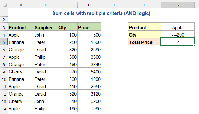
Примените любую из приведенных ниже формул в пустую ячейку и нажмите Enter ключ для возврата результата:

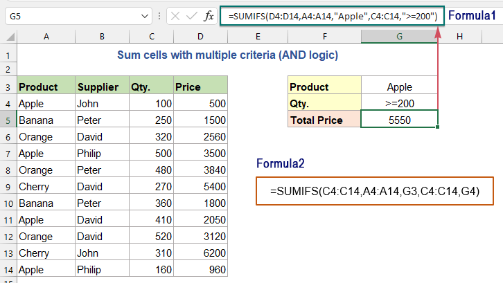
=SUMIFS(D4:D14,A4:A14,«Apple»,C4:C14,«>=200»)           (Type the criteria manually)
=SUMIFS(C4:C14,A4:A14,G3,C4:C14,G4)                           (Use cell references)

---

Пояснение к формуле:

=SUMIFS(D4:D14,A4:A14,»Apple»,C4:C14,»>=200″)

• Диапазон A4: A14 проверяет наличие продукта «Apple», а диапазон C4: C14 извлекает все количества, превышающие или равные 200, затем функция СУММЕСЛИМН суммирует только совпавшие ячейки из диапазона D4: D14.

---

Используемая относительная функция:

---

Другие статьи:

Date yes Add (Subtract) Days to a Date Concatenate Dates Convert Date to Number Convert Date to Text Month Name to Number Create Date Range from Dates Day Number of Year Month Name from Date First Day of Month Add (Subtract) Weeks to a Date If Functions with Dates Max Date Number of Days Between Dates Number of Days in a Month Number of Weeks Between Dates Number of Years Between Dates Split Date & Time into Separate Cells Countdown Remaining Days Insert Dates Random Date Generator Using Dynamic Ranges — Year to Date Values Add (Subtract) Years to a Date Date Formula Examples Extract Day from Date Get Day Name from Date Count Days Left in Month / Year Count Workdays Left in Month / Year Get Last Day of Month Last Business Day of Month / Year Number of Work / Business Days in Month Weekday Abbreviations Auto Populate Dates Number of Months Between Dates Quarter from a Date Years of Service Change Date Format Compare Dates Time yes Add (Subtract) Hours to Time Add (Subtract) Minutes to Time Add (Subtract) Seconds to Time Add Up time (Total Time) Time Differences Change Time Format Convert Minutes to Hours Convert Time to Decimal Convert Time to Hours Convert Time to Minutes Convert Time to Seconds Military Time Round Time to Nearest 15 Minutes Overtime Calculator Number of Hours Between Times Convert Seconds to Minutes, Hours, or Time Count Hours Worked Time Differences Time Format — Show Minutes Seconds Text yes Add Commas to Cells Get First Word from Text Capitalize First Letter Clean & Format Phone #s Remove Extra Trailing / Leading Spaces Add Spaces to Cell Assign Number Value to Text Combine Cells with Comma Combine First and Last Names Convert Text String to Date Convert Text to Number Extract Text From Cell Get Last Word Remove Unwated Characters Extract Text Before or After Character How to Split Text String by Space, Comma, & More Remove Special Characters Remove First Characters from Left Substitute Multiple Values Switch First & Last Names w/ Commas Remove Specific Text from a Cell Extract Text Between Characters (Ex. Parenthesis) Add Leading Zeros to a Number Remove Line Breaks from Text Remove all Numbers from Text Reverse Text Remove Non-Numeric Characters Remove Last Character(s) From Right Separate First and Last Names Separate Text & Numbers Round yes Round Formulas Round Price to Nearest Dollar or Cent Round to Nearest 10, 100, or 1000 Round to Nearest 5 or .5 Round Percentages Round to Significant Figures Count yes Count Blank and Non-blank Cells Count Cells Between Two Numbers Count Cells not Equal to Count if Cells are in Range Count Times Word Appears in Cell Count Words in Cell Count Specific Characters in Column Count Total Number of Characters in Column Count Cells that Equal one of two Results Count Cells that do not Contain Count Cells that Contain Specific Text Count Unique Values in Range Countif — Multiple Criteria Count Total Number of Cells in Range Count Cells with Any Text Count Total Cells in a Table Lookup yes Two Dimensional VLOOKUP VLOOKUP Simple Example Vlookup — Multiple Matches Case Sensitive Lookup Case Sensitive VLOOKUP Sum if — VLOOKUP Case Sensitive Lookup Case Sensitive VLOOKUP Find Duplicates w/ VLOOKUP or MATCH INDEX MATCH MATCH Lookup — Return Cell Address (Not Value) Lookup Last Value in Column or Row Reverse VLOOKUP (Right to Left) Risk Score Bucket with VLOOKUP Sum with a VLOOKUP Function VLOOKUP & INDIRECT VLOOKUP Concatenate VLOOKUP Contains (Partial Match) 17 Reasons Why Your XLOOKUP is Not Working Double (Nested) XLOOKUP — Dynamic Columns IFERROR (& IFNA) XLOOKUP Lookup Min / Max Value Nested VLOOKUP Top 11 Alternatives to VLOOKUP (Updated 2022!) VLOOKUP – Dynamic Column Reference VLOOKUP – Fix #N/A Error VLOOKUP – Multiple Sheets at Once VLOOKUP & HLOOKUP Combined VLOOKUP & MATCH Combined VLOOKUP Between Worksheets or Spreadsheets VLOOKUP Duplicate Values VLOOKUP Letter Grades VLOOKUP Return Multiple Columns VLOOKUP Returns 0? Return Blank Instead VLOOKUP w/o #N/A Error XLOOKUP Multiple Sheets at Once XLOOKUP Between Worksheets or Spreadsheets XLOOKUP by Date XLOOKUP Duplicate Values XLOOKUP Multiple Criteria XLOOKUP Return Multiple Columns XLOOKUP Returns 0? Return Blank Instead XLOOKUP Text XLOOKUP with IF XLOOKUP With If Statement Misc. yes Sort Multiple Columns Use Cell Value in Formula Percentage Change Between Numbers Percentage Breakdown Rank Values Add Spaces to Cell CAGR Formula Average Time Decimal Part of Number Integer Part of a Number Compare Items in a List Dealing with NA() Errors Get Worksheet Name Wildcard Characters Hyperlink to Current Folder Compound Interest Formula Percentage Increase Create Random Groups Sort with the Small and Large Functions Non-volatile Function Alternatives Decrease a Number by a Percentage Calculate Percent Variance Profit Margin Calculator Convert Column Number to Letter Get Full Address of Named Range Insert File Name Insert Path Latitute / Longitude Functions Replace Negative Values Reverse List Range Convert State Name to Abbreviation Create Dynamic Hyperlinks Custom Sort List with Formula Data Validation — Custom Formulas Dynamic Sheet Reference (INDIRECT) Reference Cell in Another Sheet or Workbook Get Cell Value by Address Get Worksheet Name Increment Cell Reference List Sheet Names List Skipped Numbers in Sequence Return Address of Max Value in Range Search by Keywords Select Every Other (or Every nth) Row Basics yes Cell Reference Basics — A1, R1C1, 3d, etc. Add Up (Sum) Entire Column or Row Into to Dynamic Array Formulas Conversions yes Convert Time Zones Convert Celsius to Fahrenheit Convert Pounds to Kilograms Convert Time to Unix Time Convert Feet to Meters Convert Centimeters to Inches Convert Kilometers to Miles Convert Inches to Feet Convert Date to Julian Format Convert Column Letter to Number Tests yes Test if a Range Contains any Text Test if any Cell in Range is Number Test if a Cell Contains a Specific Value Test if Cell Contains Any Number Test if Cell Contains Specific Number Test if Cell is Number or Text If yes Percentile If Subtotal If Sumproduct If Large If and Small If Median If Concatentate If Max If Rank If TEXTJOIN If Sum yes Sum if — Begins With / Ends With Sum if — Month or Year to Date Sum if — By Year Sum if — Blank / Non-Blank Sum if — Horizontal Sum Count / Sum If — Cell Color INDIRECT Sum Sum If — Across Multiple Sheets Sum If — By Month Sum If — Cells Not Equal To Sum If — Not Blank Sum if — Between Values Sum If — Week Number Sum Text Sum if — By Category or Group Sum if — Cell Contains Specific Text (Wildcards) Sum if — Date Rnage Sum if — Dates Equal Sum if — Day of Week Sum if — Greater Than Sum if — Less Than Average yes Average Non-Zero Values Average If — Not Blank Average — Ignore 0 Average — Ignore Errors Math yes Multiplication Table Cube Roots nth Roots Square Numbers Square Roots Calculations yes Calculate a Ratio Calculate Age KILLLLLLL Calculate Loan Payments GPA Formula Calculate VAT Tax How to Grade Formulas Find yes Find a Number in a Column / Workbook Find Most Frequent Numbers Find Smallest n Values Find nth Occurance of Character in Text Find and Extract Number from String Find Earliest or Latest Date Based on Criteria Find First Cell with Any Value Find Last Row Find Last Row with Data Find Missing Values Find Largest n Values Most Frequent Number Conditional Formatting yes Conditional Format — Dates & Times Conditional Format — Highlight Blank Cells New Functions XLOOKUP Replaces VLOOKUP, HLOOKUP, and INDEX / MATCH Logical yes AND Checks whether all conditions are met. TRUE/FALSE IF If condition is met, do something, if not, do something else. IFERROR If result is an error then do something else. NOT Changes TRUE to FALSE and FALSE to TRUE. OR Checks whether any conditions are met. TRUE/FALSE XOR Checks whether one and only one condition is met. TRUE/FALSE Lookup & Reference yes FALSE The logical value: FALSE. TRUE The logical value: TRUE. ADDRESS Returns a cell address as text. AREAS Returns the number of areas in a reference. CHOOSE Chooses a value from a list based on it’s position number. COLUMN Returns the column number of a cell reference. COLUMNS Returns the number of columns in an array. HLOOKUP Lookup a value in the first row and return a value. HYPERLINK Creates a clickable link. INDEX Returns a value based on it’s column and row numbers. INDIRECT Creates a cell reference from text. LOOKUP Looks up values either horizontally or vertically. MATCH Searches for a value in a list and returns its position. OFFSET Creates a reference offset from a starting point. ROW Returns the row number of a cell reference. ROWS Returns the number of rows in an array. TRANSPOSE Flips the oriention of a range of cells. VLOOKUP Lookup a value in the first column and return a value. Date & Time yes DATE Returns a date from year, month, and day. DATEDIF Number of days, months or years between two dates. DATEVALUE Converts a date stored as text into a valid date DAY Returns the day as a number (1-31). DAYS Returns the number of days between two dates. DAYS360 Returns days between 2 dates in a 360 day year. EDATE Returns a date, n months away from a start date. EOMONTH Returns the last day of the month, n months away date. HOUR Returns the hour as a number (0-23). MINUTE Returns the minute as a number (0-59). MONTH Returns the month as a number (1-12). NETWORKDAYS Number of working days between 2 dates. NETWORKDAYS.INTL Working days between 2 dates, custom weekends. NOW Returns the current date and time. SECOND Returns the second as a number (0-59) TIME Returns the time from a hour, minute, and second. TIMEVALUE Converts a time stored as text into a valid time. TODAY Returns the current date. WEEKDAY Returns the day of the week as a number (1-7). WEEKNUM Returns the week number in a year (1-52). WORKDAY The date n working days from a date. WORKDAY.INTL The date n working days from a date, custom weekends. YEAR Returns the year. YEARFRAC Returns the fraction of a year between 2 dates. Engineering yes CONVERT Convert number from one unit to another. Financial yes FV Calculates the future value. PV Calculates the present value. NPER Calculates the total number of payment periods. PMT Calculates the payment amount. RATE Calculates the interest Rate. NPV Calculates the net present value. IRR The internal rate of return for a set of periodic CFs. XIRR The internal rate of return for a set of non-periodic CFs. PRICE Calculates the price of a bond. YIELD Calculates the bond yield. INTRATE The interest rate of a fully invested security. Information yes CELL Returns information about a cell. ERROR.TYPE Returns a value representing the cell error. ISBLANK Test if cell is blank. TRUE/FALSE ISERR Test if cell value is an error, ignores #N/A. TRUE/FALSE ISERROR Test if cell value is an error. TRUE/FALSE ISEVEN Test if cell value is even. TRUE/FALSE ISFORMULA Test if cell is a formula. TRUE/FALSE ISLOGICAL Test if cell is logical (TRUE or FALSE). TRUE/FALSE ISNA Test if cell value is #N/A. TRUE/FALSE ISNONTEXT Test if cell is not text (blank cells are not text). TRUE/FALSE ISNUMBER Test if cell is a number. TRUE/FALSE ISODD Test if cell value is odd. TRUE/FALSE ISREF Test if cell value is a reference. TRUE/FALSE ISTEXT Test if cell is text. TRUE/FALSE N Converts a value to a number. NA Returns the error: #N/A. TYPE Returns the type of value in a cell. Math yes ABS Calculates the absolute value of a number. AGGREGATE Define and perform calculations for a database or a list. CEILING Rounds a number up, to the nearest specified multiple. COS Returns the cosine of an angle. DEGREES Converts radians to degrees. DSUM Sums database records that meet certain criteria. EVEN Rounds to the nearest even integer. EXP Calculates the exponential value for a given number. FACT Returns the factorial. FLOOR Rounds a number down, to the nearest specified multiple. GCD Returns the greatest common divisor. INT Rounds a number down to the nearest integer. LCM Returns the least common multiple. LN Returns the natural logarithm of a number. LOG Returns the logarithm of a number to a specified base. LOG10 Returns the base-10 logarithm of a number. MOD Returns the remainder after dividing. MROUND Rounds a number to a specified multiple. ODD Rounds to the nearest odd integer. PI The value of PI. POWER Calculates a number raised to a power. PRODUCT Multiplies an array of numbers. QUOTIENT Returns the integer result of division. RADIANS Converts an angle into radians. RAND Calculates a random number between 0 and 1. RANDBETWEEN Calculates a random number between two numbers. ROUND Rounds a number to a specified number of digits. ROUNDDOWN Rounds a number down (towards zero). ROUNDUP Rounds a number up (away from zero). SIGN Returns the sign of a number. SIN Returns the sine of an angle. SQRT Calculates the square root of a number. SUBTOTAL Returns a summary statistic for a series of data. SUM Adds numbers together. SUMIF Sums numbers that meet a criteria. SUMIFS Sums numbers that meet multiple criteria. SUMPRODUCT Multiplies arrays of numbers and sums the resultant array. TAN Returns the tangent of an angle. TRUNC Truncates a number to a specific number of digits. Stats yes AVERAGE Averages numbers. AVERAGEA Averages numbers. Includes text & FALSE =0, TRUE =1. AVERAGEIF Averages numbers that meet a criteria. AVERAGEIFS Averages numbers that meet multiple criteria. CORREL Calculates the correlation of two series. COUNT Counts cells that contain a number. COUNTA Count cells that are non-blank. COUNTBLANK Counts cells that are blank. COUNTIF Counts cells that meet a criteria. COUNTIFS Counts cells that meet multiple criteria. FORECAST Predict future y-values from linear trend line. FREQUENCY Counts values that fall within specified ranges. GROWTH Calculates Y values based on exponential growth. INTERCEPT Calculates the Y intercept for a best-fit line. LARGE Returns the kth largest value. LINEST Returns statistics about a trendline. MAX Returns the largest number. MEDIAN Returns the median number. MIN Returns the smallest number. MODE Returns the most common number. PERCENTILE Returns the kth percentile. PERCENTILE.INC Returns the kth percentile. Where k is inclusive. PERCENTILE.EXC Returns the kth percentile. Where k is exclusive. QUARTILE Returns the specified quartile value. QUARTILE.INC Returns the specified quartile value. Inclusive. QUARTILE.EXC Returns the specified quartile value. Exclusive. RANK Rank of a number within a series. RANK.AVG Rank of a number within a series. Averages. RANK.EQ Rank of a number within a series. Top Rank. SLOPE Calculates the slope from linear regression. SMALL Returns the kth smallest value. STDEV Calculates the standard deviation. STDEV.P Calculates the SD of an entire population. STDEV.S Calculates the SD of a sample. STDEVP Calculates the SD of an entire population TREND Calculates Y values based on a trendline. Text yes CHAR Returns a character specified by a code. CLEAN Removes all non-printable characters. CODE Returns the numeric code for a character. CONCATENATE Combines text together. DOLLAR Converts a number to text in currency format. EXACT Test if cells are exactly equal. Case-sensitive. TRUE/FALSE FIND Locates position of text within a cell.Case-sensitive. LEFT Truncates text a number of characters from the left. LEN Counts number of characters in text. LOWER Converts text to lower case. MID Extracts text from the middle of a cell. PROPER Converts text to proper case. REPLACE Replaces text based on it’s location. REPT Repeats text a number of times. RIGHT Truncates text a number of characters from the right. SEARCH Locates position of text within a cell.Not Case-sensitive. SUBSTITUTE Finds and replaces text. Case-sensitive. TEXT Converts a value into text with a specific number format. TRIM Removes all extra spaces from text. UPPER Converts text to upper case. VALUE Converts a number stored as text into a number.

This article explains how to use the SUMIFS function in Excel 2019, 2016, 2013, 2010, Excel for Microsoft 365, Excel 2019 for Mac, Excel 2016 for Mac, Excel for Mac 2011, and Excel Online.

Thanks for letting us know!