Excel formatting dates in formulas - Word и Excel - помощь в работе с программами

Updated 12/16/22: Stay up to date on the latest from Excel and download Excel templates today.

Date functions in Microsoft Excel make it possible to perform date calculations, like addition or subtraction, resulting in automated or semi-automated worksheets. The NOW function, which calculates values based on the current date and time, is a great example of this.

Taking this functionality a step further, when you mix date functions with conditional formatting, you can create spreadsheets that display date alerts automatically when a deadline is near or differentiates between types of days, like weekends and weekdays.

Get a better picture of your data.

The basics of conditional formatting for dates

To find conditional formatting for dates, go to:

Home > Conditional Formatting > Highlight Cell Rules > A Date Occurring.

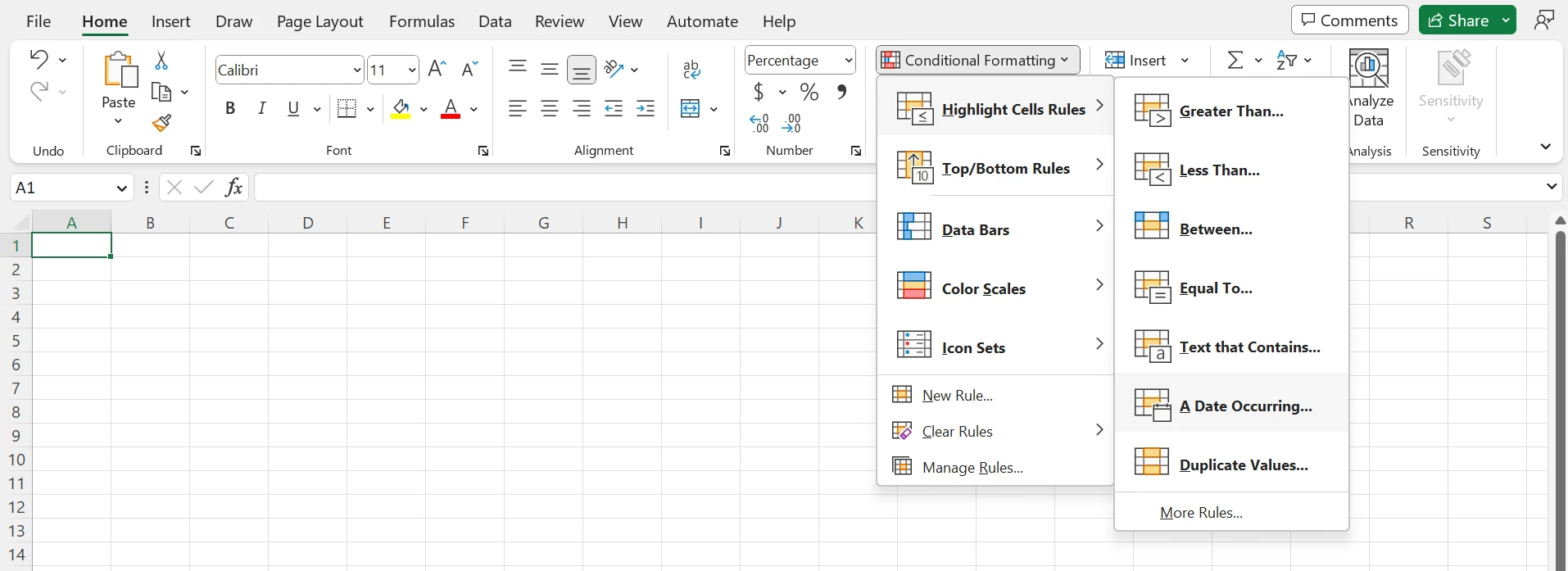
You can select the following date options, ranging from yesterday to next month:

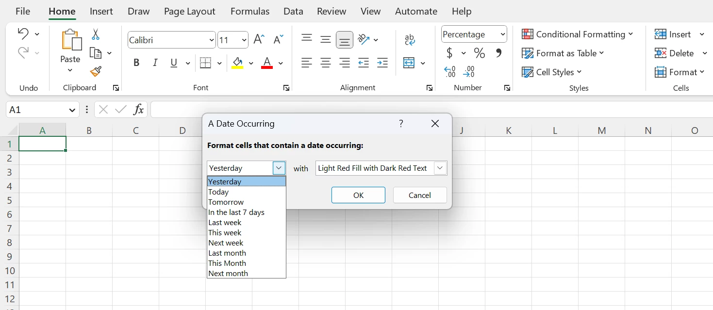
These 10 date options generate rules based on the current date. If you need to create rules for other dates (e.g., greater than a month from the current date), you can create your own new rule.

Below are step-by-step instructions for a few of my favorite conditional formats for dates.

Highlighting weekends

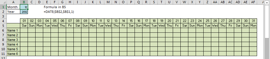
When you design an automated calendar you don’t need to color the weekends yourself. With the conditional formatting tool, you can automatically change the colors of weekends by basing the format on the WEEKDAY function. Assume that you have the date table—a calendar without conditional formatting:

To change the color of the weekends, open the menu Conditional Formatting > New Rule.

In the next dialog box, select the menu Use a formula to determine which cell to format.

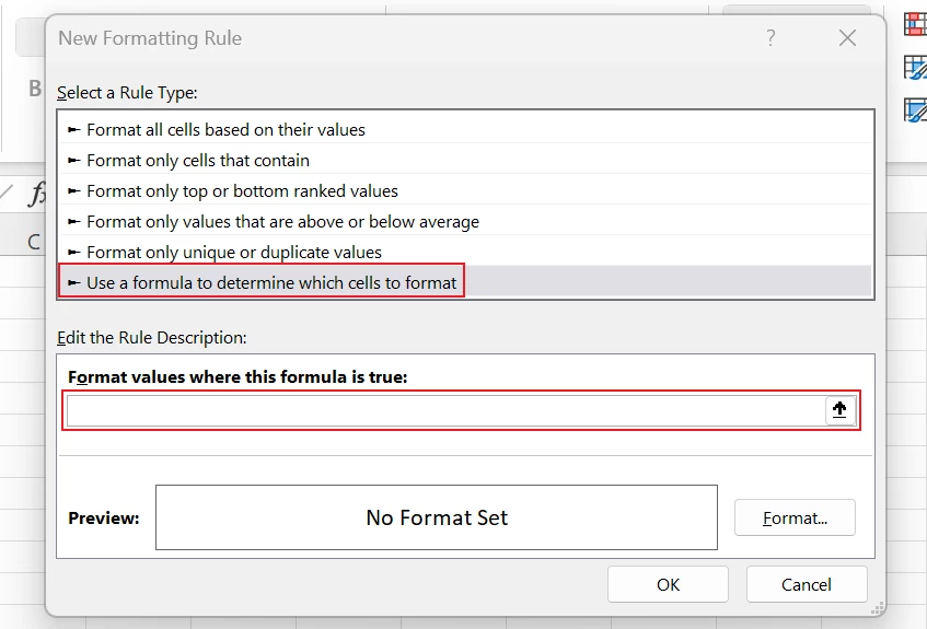
In the text box Format values where this formula is true, enter the following WEEKDAY formula to determine whether the cell is a Saturday (6) or Sunday (7):

=WEEKDAY(B$5,2)>5

Parameter 2 means Saturday = 6 and Sunday = 7. This parameter is very useful to test for weekends.

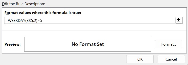
Note: In this case, you must lock the reference of the row so that the conditional format will work correctly in the other cells in this table.

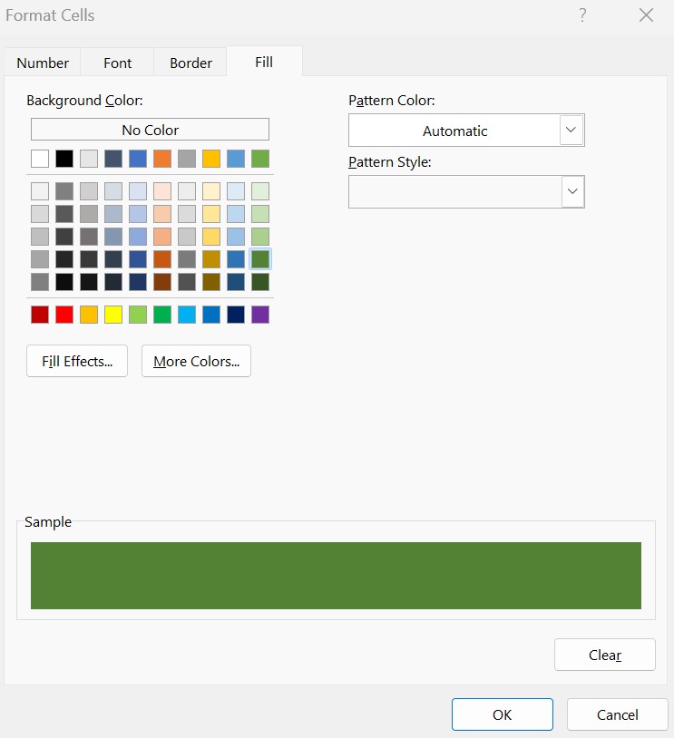
Then, customize the format of your condition by clicking on the Format button and you choose a fill color (orange in this example).

format numbers as dates <br>or times in Excel

Learn more

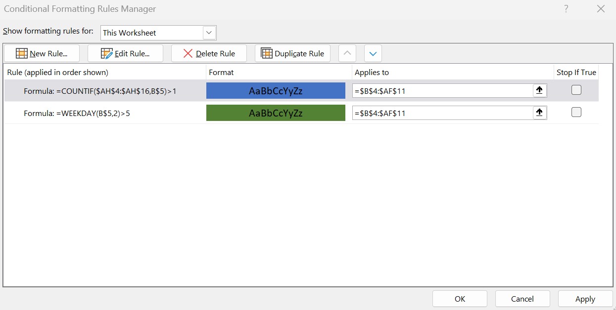
Click OK, then open Conditional Formatting> Manage Rules.

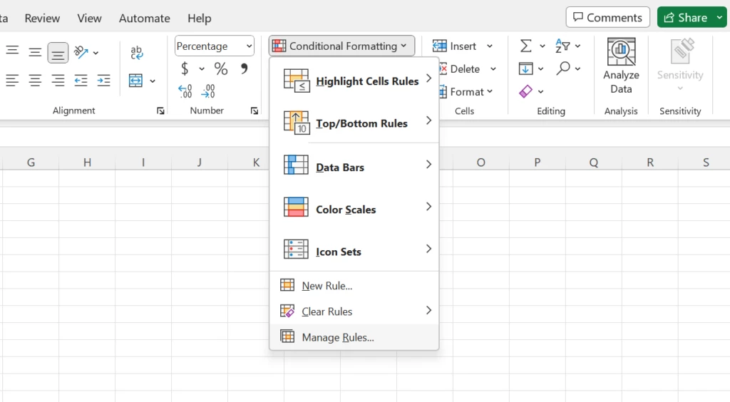
Select This Worksheet to see the worksheet rules instead of the default selection. In Applies to, change the range that corresponds to your initial selection when creating your rules to extend it to the whole column.

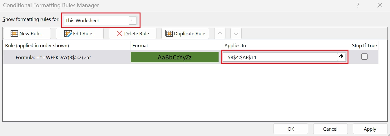
Now you will see a different color for the weekends. Note: This example shows the result in the Excel Web App.

Highlighting holidays

To enrich the previous workbook, you could also color-code holidays. To do that, you need a column with the holidays you’d like to highlight in your workbook (but not necessarily in the same sheet). In our example, we have US public holidays in column AH (as related to the year in cell B2).

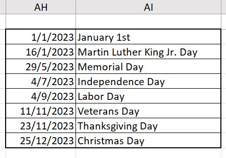
Again, open the menu Conditional Formatting > New Rule. In this case, we use the formula COUNTIF in order to count if the number of public holidays in the current month is greater than 1.

=COUNTIF($AH$4:$AH$16,B$5)>1

Then, in the dialog box Manage Rules, select the range B4:AF11. If you want to highlight the holidays over the weekends, you move the public holiday rule to the top of the list.

This example in the Excel Web App shows the result. Change the value of the month and the year to see how the calendar has a different format.

Highlighting delays

In case we want to change the color of cells based on our approach on a date again, we will use conditional formatting to make it work for us.

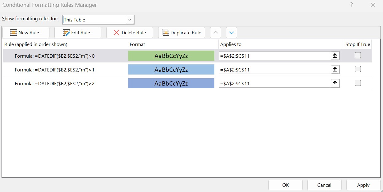
In the following example, we show:

Yellow dates between 1 and 2 months.
Orange dates between 2 and 3 months.
Purple dates more than 3 months.

We then construct three rules of conditional formatting using the formula DATEDIF. Respectively for the three cases the following formulas:

=DATEDIF($B2,$E$2,”m”)>0

=DATEDIF($B2,$E$2,”m”)>1

=DATEDIF($B2,$E$2,”m”)>2

In the Excel Web App, try changing some dates to experiment with the result.

Task management in Microsoft 365

Collaborate on shared Office documents, including Excel, Word, and PowerPoint.

Color scales

Rather than choose a different color set for each period in our timeframe, we will work with the option of color scales to color our cells.

First, go into a new column (column E) and calculate the difference in the number of days in a year again with the DATEDIF formula and the parameter “yd”.

=DATEDIF($D2,TODAY(),”yd”)

Then choose the menu Conditional Formatting> New Rule option Format all cells based on their value and choose the following options:

Scale = 3 colors
Minimum = 0 Green
Midpoint = 10 White
Maximum = 30 Blue

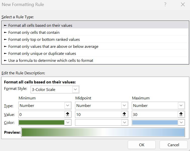
The result is a gradient color scale with nuances from green to white and through blue. The closer to 0 the more green, the closer to 10 the more white, and the closer to 30 the more blue. In the Excel app, try changing some dates to experiment with the result.

Learn more

Explore Microsoft Excel today.

Additional resources:

Read more about the DATE function.
Read how to format numbers as dates and times.

Источник

If you are storing dates in Excel worksheets, the default format picked by the Excel is the format set in Control Panel. So, if your control panel setting is “M/d/yyyy”, the Excel will format the 2nd Feb 2010 date as follows:

2/2/2010

If you require displaying the date like 2-Feb-2010 or August 1, 2015, etc. as entering dates you may change the settings in Excel easily.

In case you require permanently changing the date format that applies to current as well as future work in Excel, you should change this in the control panel.

If you try entering a date like this: 20/2/2010 then Excel will take it as text because you provided day first for the default M/d/yyyy format.

For the current worksheet, you may set the date formatting in different ways as described in the following section with examples.

Related Learning: Add / Subtract Dates in Excel

First Way: Change the date format by “Format Cell” option

The first way I am going to show you for changing the date format in Excel is using the “Format Cells” option. Follow these steps:

Step 1:

Right click on a cell or multiple cells where you require changing the date format. For the demo, I have entered a few dates and selected all:

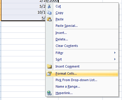
Click the “Format Cells” option that should open the Format Cells dialog. You may also press the Ctrl+1 for opening this dialog in Windows. For Mac, the short key is Control+1 or Command+1.

Step 2:

In the Format Cells dialog, the Number tab should be pre-selected. If not, press Number tab. Under the Category, select Date. Towards the right side, you can see Type.

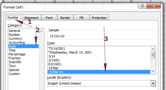
For the demo, I have selected 14-Mar-01 format and press OK. The resultant sheet after modifying date format is:

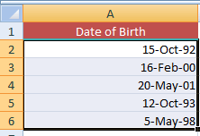
You are done!

An example of Mon-year format

The following example displays the dates in Mon-Year format e.g. Oct-92. For that, open the “Format Cells” dialog again –> Number –> Date and select Mar-01 format.

The above sheet displays the same dates as shown below:

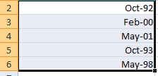
Similarly, you may choose any date format as per the requirement of your scenario.

Interesting Topic: How to calculate age in Excel

Change date format by locale/location

If you wish to display the dates based on other languages then you may use the Locale (location) option in the “Format Cells” dialog.

See the following Excel sheet where I set the Arabic(UAE) option and one of its type:

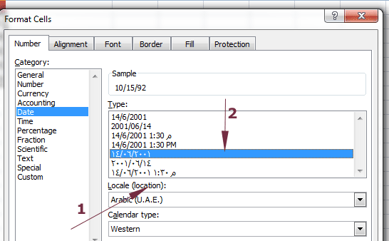
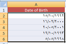
The resultant sheet for the same dates as in the above examples:

Similarly, you may choose the following locale:

Bashkir (Russia)
Chinese (Simplified, Singapore)
Corsican (France)
Danish (Denmark)
Various options for English
Hindi (India)
Japanese (Japan)
And many more

Customizing the date format

By using the date formatting codes, you may customize the dates in a flexible way. For example, displaying the short month name (Jan, Feb) by using “mmm” or full month name by “mmmm”.

Similarly, showing the day names of the Week (Sun, Mon) by ddd or full names (Sunday, Monday) by dddd formatting code.

First, have look at an example of customizing the date which is followed by the list of date formatting codes.

Select and right click on date cells that you want to customize and go to “Format Cells”. Under the Number –> Category, select Date and choose the closest format you wish to display e.g. “Mar 14, 2001”.

Under the Category, press Custom now and towards the right side, you should see Type with various options. Either choose a format from the available list or enter the formatting code as required in the text box under Type.

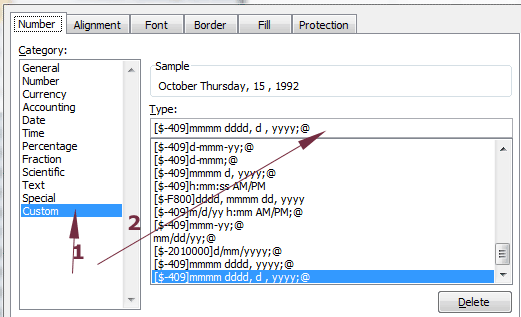
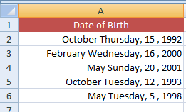
For the example, I entered the “[$-409]mmmm dddd, d , yyyy;@” and see the resultant sheet:

List of formatting codes in Excel

Following is the formatting code list that you may use to customize the dates:

Day Codes

d – for the day as 1-31
dd – for the day as 01-31
ddd – Sun, Mon, Tue
dddd – Sunday, Monday, Tuesday etc.

Month Codes

m – for Months as 1-12
mm – 01-12
mmm – Apr, May, Jun etc.
mmmm – April, May, June, July etc.
mmmmm – Month as the first letter of the month

Year Codes

yy – 00-99
yyyy – 2000, 2002, 2010 etc.

You may also want to learn: Convert Number and Date to Text

Quick way of displaying dates in default short and long formats

If you need to display dates in the short or long format with default settings, you may do it by following this:

Select the dates you wish to format in short/long date formats. For that, I chose the above example dates that were formatted in the custom format (see the last graphic):

Now, go to the Home tab and in the Number group, click the Number Format box as shown below:

Press the Short Date or Long Date format.

Changing date format in Excel by TEXT function

The Excel TEXT function can also be used for formatting dates. The TEXT function takes two arguments as shown below:

=TEXT(Value to convert into text, “Formatting code “)

Where the first argument can be a date cell, a number etc.

The second argument should sound familiar now; the formatting code that we just learned.

The TEXT function for formatting dates can particularly be useful if you want to keep the original date column in place and displaying another date-set based on those dates.

An example of Full month, day and year formatting example

For the example, the A column cells are assigned the Date of Birth dates in default format (US English) i.e. M/d/yyyy.

The corresponding B cells will display the dates in full month name, day and year in four digits format.

The TEXT formula:

=TEXT(A2,«mmmm dd, yyyy»)

The resultant sheet with formatted dates:

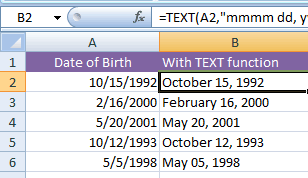
I have written the formula in the B2 cell only and copied to B6 cell as follows.

After you get the result in B2 cell by writing the above formula, bring the mouse over the right bottom of the B2 cell. As + sign appears with solid line, drag the handle till B6 and formula should be copied to other cells. The Excel will update the corresponding A cells with respect to B cells automatically.

How to use the DATEDIF function in Excel

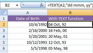
Formatting dates in d, mmm, yy by TEXT function

The following example displays the dates in day with leading zero (01-12), short month name and year in two-digit format.

The TEXT formula:

The resultant sheet:

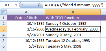
Displaying the day name as well

See the example below where day name (Sunday, Monday etc.) is also displayed along with day without leading zero, full month name and year in four digits.

The formula:

=TEXT(A2,«dddd d mmmm, yyyy»)

The dates after formatting:

The TEXT function is more than formatting dates; this is just one usage that I explained in above section. You may learn more about this function: The TEXT function in Excel

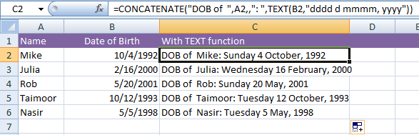
The example of concatenating formatted dates

Let us get more comfortable with date formatting and create more useful text strings as a result of joining different cells with constant literals.

In the example below, column A contains Names and column B date of births. In column C, I will use the CONCATENATE function where a text string is used and corresponding A and B cells are joined in the formula as follows:

=CONCATENATE(«DOB of «,A2,,«: «,TEXT(B2,«dddd d mmmm, yyyy»))

This is what we get:

Formatting dates specific to language by TEXT function

As we have seen in the custom date formatting example, you can display Locale specific date style. I showed an example of displaying dates in Arabic style by using custom date option in “Format cells” dialog.

You may also specify the language code in the TEXT function for displaying dates based on locales.

See the following example where I displayed dates in various languages by using TEXT function.

The resultant sheet:

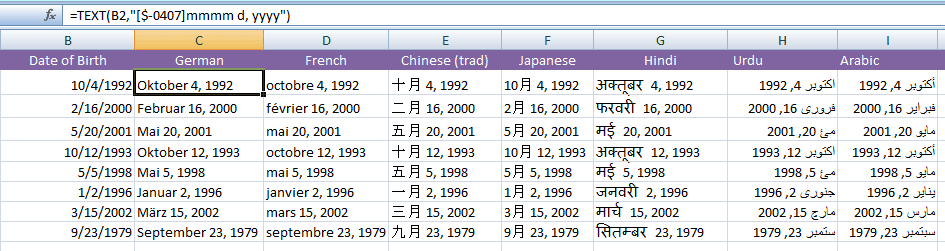
The following formulas are used for different languages:

For German:

=TEXT(B2,«[$-0407]mmmm d, yyyy»)

French:

=TEXT(B2,«[$-0040C]mmmm d, yyyy»)

Chinese (Traditional):

=TEXT(B2,«[$-0804]mmmm d, yyyy»)

Japanese:

=TEXT(B2,«[$-0411]mmmm d, yyyy»)

Arabic:

=TEXT(B2,«[$-0401]mmmm d, yyyy»)

For Hindi:

=TEXT(B2,«[$-0439]mmmm d, yyyy»)

Urdu:

=TEXT(B2,«[$-0420]mmmm d, yyyy»)

List of language codes

Following is the list of language codes that you may use in the TEXT function for locale-specific date formatting:

Lang. Code Language

042B Armenian
044D Assamese
082C Azeri (Cyrillic)
042C Azeri (Latin)
042D Basque
0423 Belarusian
0445 Bengali
0402 Bulgarian
0804 Chinese (Simplified)
0404 Chinese (Traditional)
041A Croatian
0405 Czech
0406 Danish
0413 Dutch
0C09 English (Australian)
1009 English (Canadian)
0809 English (U.K.)
0409 English (U.S.)
0464 Filipino
040B Finnish
040C French
0C0C French (Canadian)
0462 Frisian
0467 Fulfulde
0456 Galician
0437 Georgian
0407 German
0C07 German (Austrian)
0807 German (Swiss)
0408 Greek
0447 Gujarati
040D Hebrew
0439 Hindi
040E Hungarian
0421 Indonesian
0410 Italian
0411 Japanese
044B Kannada
0460 Kashmiri (Arabic)
0412 Korean
0476 Latin
0426 Latvian
0427 Lithuanian
042F Macedonian FYROM
043E Malay
044C Malayalam
043A Maltese
0458 Manipuri
044E Marathi
0450 Mongolian
0461 Nepali
0414 Norwegian Bokmal
0463 Pashto
0429 Persian
0415 Polish
0416 Portuguese (Brazil)
0816 Portuguese (Portugal)
0446 Punjabi
0418 Romanian
0419 Russian
044F Sanskrit
0C1A Serbian (Cyrillic)
081A Serbian (Latin)
0459 Sindhi
045B Sinhalese
041B Slovak
0424 Slovenian
0477 Somali
0C0A Spanish
0441 Swahili
041D Swedish
045A Syriac
0428 Tajik
045F Tamazight (Arabic)
085F Tamazight (Latin)
0449 Tamil
044A Telugu
041E Thai
041F Turkish
0442 Turkmen
0422 Ukrainian
0420 Urdu
0843 Uzbek (Cyrillic)
0443 Uzbek (Latin)
042A Vietnamese
0478 Yi
046A Yoruba

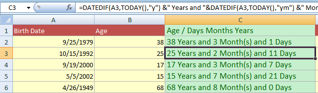
The example of calculating age in Years/Months and days

The following example uses the DATEDIF function for calculating the difference between current date and date of birth.

The current date is retrieved by using the TODAY() function. The Birth Date is stored in A column. The C column displays the formatted age in years, months and number of days.

The DATEDIF formula:

=DATEDIF(A3,TODAY(),«y») &» Years and «&DATEDIF(A3,TODAY(),«ym») &» Month(s) and « &DATEDIF(A3,TODAY(),«md») &» Days»

The resultant sheet:

For learning about the DATEDIF function, visit this tutorial: Excel DATEDIF function and formulas.

Источник

What is a date in Excel?

A date is a number! And like any number (currency, percentage, decimal, …), you can customize your date format 👍

Dates are whole numbers

Usually, when you insert a date in a cell it is displayed in the format dd/mm/yyyy or mm/dd/yyyy.

Let’s say you have the date 01/01/2016 in a cell. If you change the cell’s format to Standard, the cell displays 42370 😕🤔

Explanation of the numbering

In Excel, a date is the number of days since 01/01/1900 (the first date in Excel).

So 42370 is the number of days between 01/01/1900 and 01/01/2016.

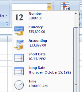
Date format

Dates can be displayed in different ways using the following 2 options (available in the Number Format dropdown in the main menu):

Short Date
Long Date

How to customize a date?

To customize a date:

Open the dialog box Custom Number (with the shortcut Ctrl + 1 or by clicking on the menu More number formats at the bottom of the number format dropdown)

In this dialog box, you select ‘Custom‘ in the Category list and write the date format code in ‘Type‘.

To format a date, you just write the parameter d, m or y a different number of times. For example,

dd/mm/yyyy will display 01/01/2016
dd mmm yyyy => 01 Jan 2016
mmmm yyyy => January 2016
dddd dd => Friday 01

In function of your language , the letter could be different:

t for «tag» (day) in German
j for «jour» (day) in French
a for «año» (year) in Spanish

Don’t write text in your cell !!!

With dates, one of the most common mistakes is to write text inside the format code (1 January 2016 for example). Never do this in Excel ⛔⛔⛔

If you do this, the contents of the cell will be Text and not a number

In Excel, text is always displayed on the left of a cell.
A number or a date is displayed on the right.

If you want to display the month in letters, just change the month format of your date.

Different examples of custom date

The following document shows you the same date but in different formats. The code for each date is in column A.

Different writing of dates according to the format code

In the following document, you can see the impact of each format on the same date.

Источник

Dates and times in Excel are stored as serial numbers and converted to human readable values on the fly using number formats. When you enter a date in Excel, you can apply a number format to display that date as you like. In a similar way, the TEXT function allows you to convert a date or time into text in a preferred format. For example, if the date January 9, 2000 is entered in cell A1, you can use TEXT to convert this date into the following text strings as follows:

=TEXT(A1,"mmm")            // "Jan"
=TEXT(A1,"dd/mm/yyyy")     // "09/01/2012"
=TEXT(A1,"dd-mmm-yy")      // "09-Jan-12"

Date format codes

Assuming a date of January 9, 2012, here is a more complete set of formatting codes for date, along with sample output.

Format code	Output
d	9
dd	09
ddd	Mon
dddd	Monday
m	1
mm	01
mmm	Jan
mmmm	January
mmmmm	J
yy	12
yyyy	2012
mm/dd/yyyy	01/09/2012
m/d/y	1/9/12
ddd, mmm d	Mon, Jan 9
mm/dd/yyyy h:mm AM/PM	01/09/2012 5:15 PM
dd/mm/yyyy hh:mm:ss	09/01/2012 17:15:00

You can use the TEXT function to convert dates or any numeric value to a fixed text format. You can explore available formats by navigating to Format Cells (Win: Ctrl + 1, Mac: Cmd + 1) and selecting various format categories in the list to the left. Also see: Excel custom number formats.

Источник

Updated on December 30, 2020

What to Know

Excel supports several pre-set options such as dates, duplicate data, and values above or below the average value of a range of cells.
You can apply different formatting options such as color or when a value meets criteria that you have pre-set.

This article explains five different ways to use conditional formatting in Excel. Instructions apply to Excel 2019, 2016, 2013, 2010; Excel for Mac, Excel for Microsoft 365, and Excel Online.

How to Use Conditional Formatting

To make conditional formatting easier, Excel supports pre-set options that cover commonly used situations, such as:

Dates
Duplicate data
Values above or below the average value in a range of cells

In the case of dates, the pre-set options simplify the process of checking your data for dates close to the current date such as yesterday, tomorrow, last week, or next month.

If you want to check for dates that fall outside of the listed options, however, customize the conditional formatting by adding your own formula using one or more of Excel’s date functions.

Check for Dates 30, 60, and 90 Days Past Due

Customize conditional formatting using formulas by setting a new rule that Excel follows when evaluating the data in a cell.

Excel applies conditional formatting in top-to-bottom order as they appear in the Conditional Formatting Rules Manager dialog box.

Even though several rules may apply to some cells, the first rule that meets the condition is applied to the cells.

This demo uses the current date, 40 days before the current date, 70 days before the current date, and 100 days before the current date to generate the results.

Check for Dates 30 Days Past Due

In a blank Excel worksheet, highlight cells C1 to C4 to select them. This is the range to which the conditional formatting rules will be applied.

Select Home > Conditional Formatting > New Rule to open the New Formatting Rule dialog box.
Choose Use a formula to determine which cells to format.
In the Format values where this formula is true text box, enter the formula:
```
=TODAY()-C1>30
```
This formula checks to see if the dates in cells C1 to C4 are more than 30 days past.
Select Format to open the Format Cells dialog box.
Select the Fill tab to see the background fill color options.
Select a background fill color.
Select the Font tab to see font format options.
Set the font color.
Select OK twice to close the dialog boxes and return to the worksheet.
The background color of cells C1 to C4 changes to the fill color chosen, even though there are no data in the cells.

Add a Rule for Dates More Than 60 days Past Due

Rather than repeat all the steps above to add the next two rules, use the Manage Rules option to add the additional rules all at once.

Highlight cells C1 to C4, if necessary.
Select Home > Conditional Formatting > Manage Rules to open the Conditional Formatting Rules Manager dialog box.
Select New Rule.
Select Use a formula to determine which cells to format.
In the Format values where this formula is true text box, enter the formula:
```
=TODAY()-C1>60
```
This formula checks to see if the dates in cells C1 to C4 are greater than 60 days past.
Select Format to open the Format Cells dialog box.
Select the Fill tab to see the background fill color options.
Select a background fill color.
Select OK twice to close the dialog box and return to the Conditional Formatting Rules Manager dialog box.

Add a Rule for Dates More Than 90 days Past Due

Highlight cells C1 to C4, if necessary.
Select Home > Conditional Formatting > Manage Rules to open the Conditional Formatting Rules Manager dialog box.
Select New Rule.
Select Use a formula to determine which cells to format.
In the Format values where this formula is true, enter the formula:
```
=TODAY()-C1>90
```
This formula checks to see if the dates in cells C1 to C4 are greater than 90 days past.
Select Format to open the Format Cells dialog box.
Select the Fill tab to see the background fill color options.
Select a background fill color.
Select OK twice to close the dialog box and return to the Conditional Formatting Rules Manager dialog box.
Select OK to close this dialog box and return to the worksheet.

The background color of cells C1 to C4 changes to the last fill color chosen.

Test the Conditional Formatting Rules

Test the conditional formatting rules in cells C1 to C4 by entering the following dates:

Enter the current date in cell C1. The cell changes to the default white background with black text since none of the conditional formatting rules apply.
Enter the following formula in cell C2:
```
=TODAY()-40
```
This formula determines which date occurs 40 days before the current date. The cell is filled with the color you selected for the conditional formatting rule for dates more than 30 days past due.
Enter the following formula in cell C3:
```
=TODAY()-70
```
This formula determines which date occurs 70 days before the current date. The cell is filled with the color you selected for the conditional formatting rule for dates more than 60 days past due.
Enter the following formula in cell C4:
```
=TODAY()-100
```
This formula determines which date occurs 100 days before the current date. The cell color changes to the color you selected for the conditional formatting rule for dates more than 90 days past due.

Thanks for letting us know!

Get the Latest Tech News Delivered Every Day

Источник