
Change the format of a cell
You can apply formatting to an entire cell and to the data inside a cell—or a group of cells. One way to think of this is the cells are the frame of a picture and the picture inside the frame is the data.

Formal Cells
-
Select the cells.
-
Go to the ribbon to select changes as Bold, Font Color, or Font Size.
Apply Excel Styles
-
Select the cells.
-
Select Home > Cell Style and select a style.
Modify an Excel Style
-
Select the cells with the Excel Style.
-
Right-click the applied style in Home > Cell Styles.
-
Select Modify > Format to change what you want.
Need more help?
You can always ask an expert in the Excel Tech Community or get support in the Answers community.
See Also
Format text in cells
Format numbers
Format a date the way you want
Need more help?
При необходимости Вы можете легко добавить к стандартным числовым форматам Excel свои собственные. Для этого выделите ячейки, к которым надо применить пользовательский формат, щелкните по ним правой кнопкой мыши и выберите в контекстном меню команду Формат ячеек (Format Cells) — вкладка Число (Number), далее — Все форматы (Custom):

В появившееся справа поле Тип: введите маску нужного вам формата из последнего столбца этой таблицы:

Как это работает…
На самом деле все очень просто. Как Вы уже, наверное, заметили, Excel использует несколько спецсимволов в масках форматов:
- 0 (ноль) — одно обязательное знакоместо (разряд), т.е. это место в маске формата будет заполнено цифрой из числа, которое пользователь введет в ячейку. Если для этого знакоместа нет числа, то будет выведен ноль. Например, если к числу 12 применить маску 0000, то получится 0012, а если к числу 1,3456 применить маску 0,00 — получится 1,35.
- # (решетка) — одно необязательное знакоместо — примерно то же самое, что и ноль, но если для знакоместа нет числа, то ничего не выводится
- (пробел) — используется как разделитель групп разрядов по три между тысячами, миллионами, миллиардами и т.д.
- [ ] — в квадратных скобках перед маской формата можно указать цвет шрифта. Разрешено использовать следующие цвета: черный, белый, красный, синий, зеленый, жёлтый, голубой.
Плюс пара простых правил:
- Любой пользовательский текст (кг, чел, шт и тому подобные) или символы (в том числе и пробелы) — надо обязательно заключать в кавычки.
- Можно указать несколько (до 4-х) разных масок форматов через точку с запятой. Тогда первая из масок будет применяться к ячейке, если число в ней положительное, вторая — если отрицательное, третья — если содержимое ячейки равно нулю и четвертая — если в ячейке не число, а текст (см. выше пример с температурой).
Ссылки по теме
- Как скрыть содержимое ячейки с помощью пользовательского формата
Learning how to customise a cell format in Excel allows you to not only format your data the way you want, but in some instances it can save you time.
Before we dive in you need to know that despite how the text appears after you’ve set your custom cell format, the underlying value is unchanged for the purpose of formulas and calculations.
How to enter an Excel custom cell format
Select the cell/s you want to format then open the Format Cells window.
- The quick way just press CTRL+1
- Or the way most people do it is to right click and select ‘Format Cells’.
- On the Number Tab select Custom from the Category list.

Note: It’s handy to have the text you want to format in the cell before you press CTRL+1 because Excel will give you a sample view of what the text is going to look like in the Format Cells window, so you can see before pressing OK, if it’s what you want.
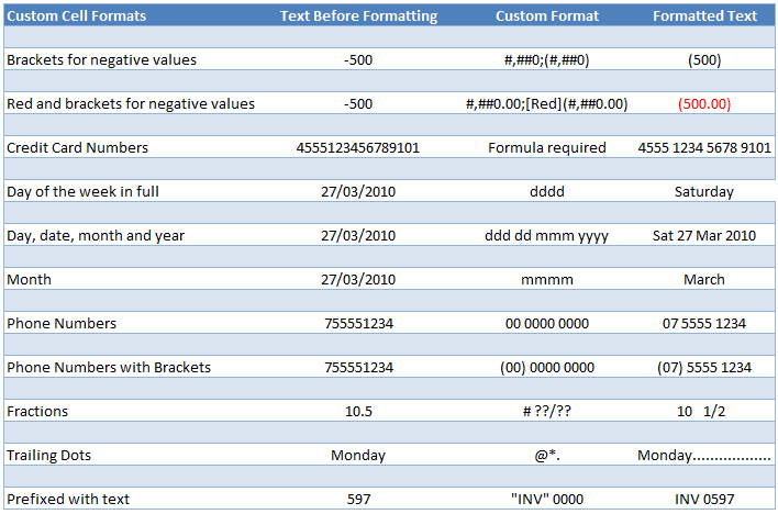
How to make your cell formats look the way you want
| Custom Cell Formats | Text Before Formatting | Custom Format | Formatted Text |
| Brackets for negative values | -500 | #,##0;(#,##0) | (500) |
| Red and brackets for negative values | -500 | #,##0.00;[Red](#,##0.00) | (500.00) |
| Day of the week in full | 27/03/2010 | dddd | Saturday |
| Day, date, month and year | 27/03/2010 | ddd dd mmm yyyy | Sat 27 Mar 2010 |
| Month | 27/03/2010 | mmmm | March |
| Phone Numbers | 755551234 | 00 0000 0000 | 07 5555 1234 |
| Phone Numbers with Brackets | 755551234 | (00) 0000 0000 | (07) 5555 1234 |
| Fractions | 10.5 | # ??/?? | 10 1/2 |
How to save time with Custom Cell Formats
1) From time to time I create a reference sheet like a contacts list, an index or even just a list of items like the one below using the custom cell format @*.

Because the text in the first column is often different lengths it can be hard for the eye to follow across. In these cases I like to use trailing dots to help the reader.
I wouldn’t dream of manually entering the dots but since I can create a custom format it’s worth it, plus I think it looks more elegant that using borders for this purpose as they can get a bit busy.
The custom cell format for trailing dots is @*. When you type in your text Excel will automatically enter the dots to fill to the end of the cell.
Tip: You’re not just limited to dots. You can have —- or **** or ____ or almost anything you want. Just replace the dot in the custom format with the character of your choice.
2) The other custom format I use regularly is prefixing my data with text. For example, I keep a record of our invoices and instead of typing ‘INV’ before each number I enter I use a custom cell format like this: “INV” 0000
Then when I type in 597 Excel converts it to INV 0597.
Tip: Replace INV with different text to suit your needs. It might be PO for purchase order, or any other text you can think of. Or make the text a suffix by changing the custom format to 0000 «INV».
Remember that even though the text appears to be INV 0597, for the purpose of formulas it’s still just a number 597.

Formatting cells for credit card numbers
You might be thinking you can use a custom format of 0000 0000 0000 0000 for credit card numbers, but you’ll find that it will only work for cards where the last number of the card is a zero! Try it out and see for yourself.
The workaround is to use a formula. This requires entering the number in one cell, and then in another cell you need to enter the following formula (assuming our credit card number is in cell A1):
=LEFT(A1,4) & " " & MID(A1,5,4) & " " & MID(A1,9,4) & " " & RIGHT(A1,4)
Note: I’ve added spaces in the formula for clarity.
Some explanation:
- The LEFT, MID and RIGHT returns text from a specified position in a cell.
- The ampersands ‘&’ join text together
- The “ “ adds a space between each group of text
[UPDATE] — You can also use this custom number format for credit cards and long phone numbers:
[<=99999999999]##########;#### #### #### ####
Thanks to MF for sharing that tip.
Enter your email address below to download the sample workbook.
By submitting your email address you agree that we can email you our Excel newsletter.
Содержание
- How to control and understand settings in the Format Cells dialog box in Excel
- Summary
- More Information
- Number Tab
- Auto Number Formatting
- Built-in Number Formats
- Custom Number Formats
- Custom cell format
- Codes for custom number formats
- Please, disable AdBlock and reload the page to continue
- How to change number, currency, or accounting format
- How to hide points on the chart axis
- How to change cells format easily
- Custom Excel number format
- How to create a custom number format in Excel
- Understanding Excel number format
- Excel formatting rules
- Digit and text placeholders
- Excel formatting tips and guidelines
- How to control the number of decimal places
- How to show a thousands separator
- Round numbers by thousand, million, etc.
- Text and spacing in custom Excel number format
- Including currency symbols in a custom number format
- How to display leading zeros with Excel custom format
- Percentages in Excel custom number format
- Fractions in Excel number format
- Create a custom Scientific Notation format
- Show negative numbers in parentheses
- Display zeroes as dashes or blanks
- Add indents with custom Excel format
- Change font color with custom number format
- Repeat characters with custom format codes
- How to change alignment in Excel with custom number format
- Apply custom number formats based on conditions
- Dates and times formats in Excel
How to control and understand settings in the Format Cells dialog box in Excel
Summary
Microsoft Excel lets you change many of the ways it displays data in a cell. For example, you can specify the number of digits to the right of a decimal point, or you can add a pattern and border to the cell. You can access and modify the majority of these settings in the Format Cells dialog box (on the Format menu, click Cells).
The «More Information» section of this article provides information about each of the settings available in the Format Cells dialog box and how each of these settings can affect the way your data is presented.
More Information
There are six tabs in the Format Cells dialog box: Number, Alignment, Font, Border, Patterns, and Protection. The following sections describe the settings available in each tab.
Number Tab
Auto Number Formatting
By default, all worksheet cells are formatted with the General number format. With the General format, anything you type into the cell is usually left as-is. For example, if you type 36526 into a cell and then press ENTER, the cell contents are displayed as 36526. This is because the cell remains in the General number format. However, if you first format the cell as a date (for example, d/d/yyyy) and then type the number 36526, the cell displays 1/1/2000.
There are also other situations where Excel leaves the number format as General, but the cell contents are not displayed exactly as they were typed. For example, if you have a narrow column and you type a long string of digits like 123456789, the cell might instead display something like 1.2E+08. If you check the number format in this situation, it remains as General.
Finally, there are scenarios where Excel may automatically change the number format from General to something else, based on the characters that you typed into the cell. This feature saves you from having to manually make the easily recognized number format changes. The following table outlines a few examples where this can occur:
| If you type | Excel automatically assigns this number format |
|---|---|
| 1.0 | General |
| 1.123 | General |
| 1.1% | 0.00% |
| 1.1E+2 | 0.00E+00 |
| 1 1/2 | # ?/? |
| $1.11 | Currency, 2 decimal places |
| 1/1/01 | Date |
| 1:10 | Time |
Generally speaking, Excel applies automatic number formatting whenever you type the following types of data into a cell:
Built-in Number Formats
Excel has a large array of built-in number formats from which you can choose. To use one of these formats, click any one of the categories below General and then select the option that you want for that format. When you select a format from the list, Excel automatically displays an example of the output in the Sample box on the Number tab. For example, if you type 1.23 in the cell and you select Number in the category list, with three decimal places, the number 1.230 is displayed in the cell.
These built-in number formats actually use a predefined combination of the symbols listed below in the «Custom Number Formats» section. However, the underlying custom number format is transparent to you.
The following table lists all of the available built-in number formats:
| Number format | Notes |
|---|---|
| Number | Options include: the number of decimal places, whether or not the thousands separator is used, and the format to be used for negative numbers. |
| Currency | Options include: the number of decimal places, the symbol used for the currency, and the format to be used for negative numbers. This format is used for general monetary values. |
| Accounting | Options include: the number of decimal places, and the symbol used for the currency. This format lines up the currency symbols and decimal points in a column of data. |
| Date | Select the style of the date from the Type list box. |
| Time | Select the style of the time from the Type list box. |
| Percentage | Multiplies the existing cell value by 100 and displays the result with a percent symbol. If you format the cell first and then type the number, only numbers between 0 and 1 are multiplied by 100. The only option is the number of decimal places. |
| Fraction | Select the style of the fraction from the Type list box. If you do not format the cell as a fraction before typing the value, you may have to type a zero or space before the fractional part. For example, if the cell is formatted as General and you type 1/4 in the cell, Excel treats this as a date. To type it as a fraction, type 0 1/4 in the cell. |
| Scientific | The only option is the number of decimal places. |
| Text | Cells formatted as text will treat anything typed into the cell as text, including numbers. |
| Special | Select one of the following from the Type box: Zip Code, Zip Code + 4, Phone Number, and Social Security Number. |
Custom Number Formats
If one of the built-in number formats does not display the data in the format that you require, you can create your own custom number format. You can create these custom number formats by modifying the built-in formats or by combining the formatting symbols into your own combination.
Before you create your own custom number format, you need to be aware of a few simple rules governing the syntax for number formats:
Each format that you create can have up to three sections for numbers and a fourth section for text.
The first section is the format for positive numbers, the second for negative numbers, and the third for zero values.
These sections are separated by semicolons.
If you have only one section, all numbers (positive, negative, and zero) are formatted with that format.
You can prevent any of the number types (positive, negative, zero) from being displayed by not typing symbols in the corresponding section. For example, the following number format prevents any negative or zero values from being displayed:
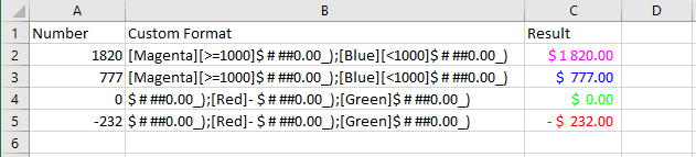
To set the color for any section in the custom format, type the name of the color in brackets in the section. For example, the following number format formats positive numbers blue and negative numbers red:
Instead of the default positive, negative and zero sections in the format, you can specify custom criteria that must be met for each section. The conditional statements that you specify must be contained within brackets. For example, the following number format formats all numbers greater than 100 as green, all numbers less than or equal to -100 as yellow, and all other numbers as cyan:
Источник
Custom cell format
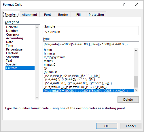
To define a custom format, follow these steps:
1. Enter sample text for the format in a cell, and then select that cell (Excel then displays the sample text in the new format, which helps see the effects of your changes).
2. Do one of the following:
- Right-click on the selection and choose Format Cells. in the popup menu:
3. In the Format Cells dialog box:
- On the Number tab, in the Category box, select the Custom item:
Codes for custom number formats
| Code | Description |
|---|---|
| General | Displays the number in general format. |
| # | Displays only significant digits and does not display insignificant zeros. |
| 0 (zero) | Displays insignificant zeros if a number has fewer digits than the zeros in the format. |
| ? | Displays a space for insignificant zeros on either side of the decimal point so that the decimal points align when formatted in a fixed-width font. |
It can also be used for fractions with different numbers of digits.
. Decimal point. % Percent symbol. , Thousand separator. E-, E+, e-, e+ Scientific notation. $, —, +, /, (, ), :, space Displays this character. * Repeats the next character to fill the full width of the column:
_ (underscore) Leaves a space equal to the width of the next character. “text” Displays text enclosed in double quotes. @ Text placeholder. [color] Displays characters in the specified color – black, blue, cyan, green, magenta, red, white , or yellow . [condition value] Custom criteria for each number format section.
Please, disable AdBlock and reload the page to continue
Today, 30% of our visitors use Ad-Block to block ads.We understand your pain with ads, but without ads, we won’t be able to provide you with free content soon. If you need our content for work or study, please support our efforts and disable AdBlock for our site. As you will see, we have a lot of helpful information to share.
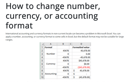
How to change number, currency, or accounting format
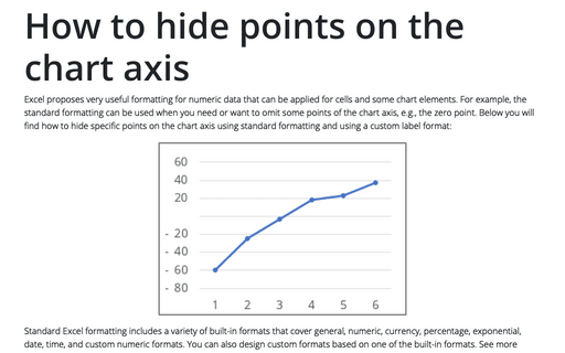
How to hide points on the chart axis
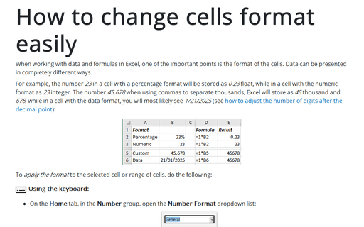
How to change cells format easily
We use cookies to personalise content and ads, to provide social media features and to analyse our traffic. We also share information about your use of our site with our social media, advertising and analytics partners who may combine it with other information you’ve provided to them or they’ve collected from your use of their services.
Источник
Custom Excel number format
 by Svetlana Cheusheva, updated on March 20, 2023
This tutorial explains the basics of the Excel number format and provides the detailed guidance to create custom formatting. You will learn how to show the required number of decimal places, change alignment or font color, display a currency symbol, round numbers by thousands, show leading zeros, and much more.
Microsoft Excel has a lot of built-in formats for number, currency, percentage, accounting, dates and times. But there are situations when you need something very specific. If none of the inbuilt Excel formats meets your needs, you can create your own number format.
Number formatting in Excel is a very powerful tool, and once you learn how to use it property, your options are almost unlimited. The aim of this tutorial is to explain the most essential aspects of Excel number format and set you on the right track to mastering custom number formatting.
How to create a custom number format in Excel
To create a custom Excel format, open the workbook in which you want to apply and store your format, and follow these steps:
- Select a cell for which you want to create custom formatting, and press Ctrl+1 to open the Format Cells dialog.
- Under Category, select Custom.
- Type the format code in the Type box.
- Click OK to save the newly created format.
Done! 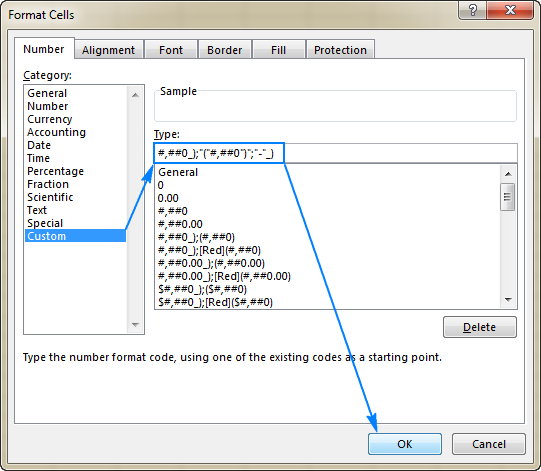
Tip. Instead of creating a custom number format from scratch, you choose a built-in Excel format close to your desired result, and customize it.
Wait, wait, but what do all those symbols in the Type box mean? And how do I put them in the right combination to display the numbers the way I want? Well, this is what the rest of this tutorial is all about 🙂
Understanding Excel number format
To be able to create a custom format in Excel, it is important that you understand how Microsoft Excel sees the number format.
An Excel number format consists of 4 sections of code, separated by semicolons, in this order:
POSITIVE; NEGATIVE; ZERO; TEXT
Here’s an example of a custom Excel format code: 
- Format for positive numbers (display 2 decimal places and a thousands separator).
- Format for negative numbers (the same as for positive numbers, but enclosed in parentheses).
- Format for zeros (display dashes instead of zeros).
- Format for text values (display text in magenta font color).
Excel formatting rules
When creating a custom number format in Excel, please remember these rules:
- A custom Excel number format changes only the visual representation, i.e. how a value is displayed in a cell. The underlying value stored in a cell is not changed.
- When you are customizing a built-in Excel format, a copy of that format is created. The original number format cannot be changed or deleted.
- Excel custom number format does not have to include all four sections.
If a custom format contains just 1 section, that format will be applied to all number types — positive, negative and zeros.
If a custom number format includes 2 sections, the first section is used for positive numbers and zeros, and the second section — for negative numbers.
A custom format is applied to text values only if it contains all four sections.
To apply the default Excel number format for any of the middle sections, type General instead of the corresponding format code.
For example, to display zeros as dashes and show all other values with the default formatting, use this format code: General; -General; «-«; General
Note. The General format included in the 2 nd section of the format code does not display the minus sign, therefore we include it in the format code.
For example, to hide zeros and negative values, use the following format code: General; ; ; General . As the result, zeros and negative value will appear only in the formula bar, but will not be visible in cells.
Digit and text placeholders
For starters, let’s learn 4 basic placeholders that you can use in your custom Excel format.
| Code | Description | Example |
| 0 | Digit placeholder that displays insignificant zeros. | #.00 — always displays 2 decimal places.
If you type 5.5 in a cell, it will display as 5.50. |
| # | Digit placeholder that only displays significant digits, without extra zeros.
That is, if a number doesn’t need a certain digit, it won’t be displayed. |
#.## — displays up to 2 decimal places.
If you type 5.5 in a cell, it will display as 5.5. If you type 5.555, it will display as 5.56. |
| ? | Digit placeholder that leaves a space for insignificant zeros on either side of the decimal point but doesn’t display them. It is often used to align numbers in a column by decimal point. | #. — displays a maximum of 3 decimal places and aligns numbers in a column by decimal point. |
| @ | Text placeholder | 0.00; -0.00; 0; [Red]@ — applies the red font color for text values. |
The following screenshot demonstrates a few number formats in action: 
As you may have noticed in the above screenshot, the digit placeholders behave in the following way:
- If a number entered in a cell has more digits to the right of the decimal point than there are placeholders in the format, the number is «rounded» to as many decimal places as there are placeholders.
For example, if you type 2.25 in a cell with #.# format, the number will display as 2.3.
All digits to the left of the decimal point are displayed regardless of the number of placeholders.
For example, if you type 202.25 in a cell with #.# format, the number will display as 202.3.
Below you will find a few more examples that will hopefully shed more light on number formatting in Excel.
| Format | Description | Input value | Display as |
| #.00 | Always display 2 decimal places. | 2 2.5 0.5556 |
2.00 2.50 .56 |
| #.## | Shows up to 2 decimal places, without insignificant zeros. | 2 2.5 0.5556 |
2. 2.5 0.56 |
| #.0# | Display a minimum of 1 and a maximum of 2 decimal places. | 2 2.205 0.555 |
2.0 2.21 .56 |
| . | Display up to 3 decimal places with aligned decimals. | 22.55 2.5 2222.5555 0.55 |
22.55 2.5 2222.556 .55 |
Excel formatting tips and guidelines
Theoretically, there are an infinite number of Excel custom number formats that you can make using a predefined set of formatting codes listed in the table below. And the following tips explain the most common and useful implementations of these format codes.
| Format Code | Description |
| General | General number format |
| # | Digit placeholder that represents optional digits and does not display extra zeros. |
| 0 | Digit placeholder that displays insignificant zeros. |
| ? | Digit placeholder that leaves a space for insignificant zeros but doesn’t display them. |
| @ | Text placeholder |
| . (period) | Decimal point |
| , (comma) | Thousands separator. A comma that follows a digit placeholder scales the number by a thousand. |
| Displays the character that follows it. | |
| » « | Display any text enclosed in double quotes. |
| % | Multiplies the numbers entered in a cell by 100 and displays the percentage sign. |
| / | Represents decimal numbers as fractions. |
| E | Scientific notation format |
| _ (underscore) | Skips the width of the next character. It’s commonly used in combination with parentheses to add left and right indents, _( and _) respectively. |
| * (asterisk) | Repeats the character that follows it until the width of the cell is filled. It’s often used in combination with the space character to change alignment. |
| [] | Create conditional formats. |
How to control the number of decimal places
The location of the decimal point in the number format code is represented by a period (.). The required number of decimal places is defined by zeros (0). For example:
- 0 or # — display the nearest integer with no decimal places.
- 0.0 or #.0 — display 1 decimal place.
- 0.00 or #.00 — display 2 decimal places, etc.
The difference between 0 and # in the integer part of the format code is as follows. If the format code has only pound signs (#) to the left of the decimal point, numbers less than 1 begin with a decimal point. For example, if you type 0.25 in a cell with #.00 format, the number will display as .25. If you use 0.00 format, the number will display as 0.25. 
How to show a thousands separator
To create an Excel custom number format with a thousands separator, include a comma (,) in the format code. For example:
- #,### — display a thousands separator and no decimal places.
- #,##0.00 — display a thousands separator and 2 decimal places.
To separate numbers with more than four digits into groups of three leaving a space between each group, use a space for the thousands separator. For example:
- # ### — rounds numbers to the nearest integer (no decimal places) separating thousands with a space.
- # ##0.00 — separate thousands with a space and display 2 decimal places.

Round numbers by thousand, million, etc.
As demonstrated in the previous tip, Microsoft Excel separates thousands by commas if a comma is enclosed by any digit placeholders — pound sign (#), question mark (?) or zero (0). If no digit placeholder follows a comma, it scales the number by thousand, two consecutive commas scale the number by million, and so on.
For example, if a cell format is #.00, and you type 5000 in that cell, the number 5.00 is displayed. For more examples, please see the screenshot below: 
Text and spacing in custom Excel number format
To display both text and numbers in a cell, do the following:
- To add a single character, precede that character with a backslash ().
- To add a text string, enclose it in double quotation marks (» «).
For example, to indicate that numbers are rounded by thousands and millions, you can add K and M to the format codes, respectively:
- To display thousands: #.00,K
- To display millions: #.00,,M
Tip. To make the number format better readable, include a space between a comma and backward slash.
The following screenshot shows the above formats and a couple more variations: 
And here is another example that demonstrates how to display text and numbers within a single cell. Supposing, you want to add the word «Increase» for positive numbers, and «Decrease» for negative numbers. All you have to do is include the text enclosed in double quotes in the appropriate section of your format code:
#.00″ Increase»; -#.00″ Decrease»; 0
Tip. To include a space between a number and text, type a space character after the opening or before the closing quote depending on whether the text precedes or follows the number, like in «Increase «. 
In addition, the following characters can be included in Excel custom format codes without the use of backslash or quotation marks:
| Symbol | Description |
| + and — | Plus and minus signs |
| ( ) | Left and right parentheses |
| : | Colon |
| ^ | Caret |
| ‘ | Apostrophe |
| Curly brackets | |
| Less-than and greater than signs | |
| = | Equal sign |
| / | Forward slash |
| ! | Exclamation point |
| & | Ampersand |
| Tilde | |
| Space character |
A custom Excel number format can also accept other special symbols such as currency, copyright, trademark, etc. These characters can be entered by typing their four-digit ANSI codes while holding down the ALT key. Here are some of the most useful ones:
| Symbol | Code | Description |
| в„ў | Alt+0153 | Trademark |
| В© | Alt+0169 | Copyright symbol |
| В° | Alt+0176 | Degree symbol |
| В± | Alt+0177 | Plus-Minus sign |
| Вµ | Alt+0181 | Micro sign |
For example, to display temperatures, you can use the format code #»В°F» or #»В°C» and the result will look similar to this: 
You can also create a custom Excel format that combines some specific text and the text typed in a cell. To do this, enter the additional text enclosed in double quotes in the 4 th section of the format code before or after the text placeholder (@), or both.
For example, to proceed the text typed in the cell with some other text, say «Shipped in«, use the following format code:
General; General; General; «Shipped in «@ 
Including currency symbols in a custom number format
To create a custom number format with the dollar sign ($), simply type it in the format code where appropriate. For example, the format $#.00 will display 5 as $5.00.
Other currency symbols are not available on most of standard keyboards. But you can enter the popular currencies in this way:
- Turn NUM LOCK on, and
- Use the numeric keypad to type the ANSI code for the currency symbol you want to display.
| Symbol | Currency | Code |
| € | Euro | ALT+0128 |
| ВЈ | British Pound | ALT+0163 |
| ВҐ | Japanese Yen | ALT+0165 |
| Вў | Cent Sign | ALT+0162 |
The resulting number formats may look something similar to this: 
If you want to create a custom Excel format with some other currency, follow these steps:
How to display leading zeros with Excel custom format
If you try entering numbers 005 or 00025 in a cell with the default General format, you would notice that Microsoft Excel removes leading zeros because the number 005 is same as 5. But sometimes, we do want 005, not 5!
The simplest solution is to apply the Text format to such cells. Alternatively, you can type an apostrophe (‘) in front of the numbers. Either way, Excel will understand that you want any cell value to be treated as a text string. As the result, when you type 005, all leading zeros will be preserved, and the number will show up as 005.
If you want all numbers in a column to contain a certain number of digits, with leading zeros if needed, then create a custom format that includes only zeros.
As you remember, in Excel number format, 0 is the placeholder that displays insignificant zeros. So, if you need numbers consisting of 6 digits, use the following format code: 000000
And now, if you type 5 in a cell, it will appear as 000005; 50 will appear as 000050, and so on: 
Tip. If you are entering phone numbers, zip codes, or social security numbers that contain leading zeros, the easiest way is to apply one of the predefined Special formats. Or, you can create the desired custom number format. For example, to properly display international seven-digit postal codes, use this format: 0000000. For social security numbers with leading zeros, apply this format: 000-00-0000.
Percentages in Excel custom number format
To display a number as a percentage of 100, include the percent sign (%) in your number format.
For example, to display percentages as integers, use this format: #%. As the result, the number 0.25 entered in a cell will appear as 25%.
To display percentages with 2 decimal places, use this format: #.00%
To display percentages with 2 decimal places and a thousands separator, use this one: #,##.00% 
Fractions in Excel number format
Fractions are special in terms that the same number can be displayed in a variety of ways. For example, 1.25 can be shown as 1 Вј or 5/5. Exactly which way Excel displays the fraction is determined by the format codes that you use.
For decimal numbers to appear as fractions, include forward slash (/) in your format code, and separate an integer part with a space. For example:
- # #/# — displays a fraction remainder with up to 1 digit.
- # ##/## — displays a fraction remainder with up to 2 digits.
- # ###/### — displays a fraction remainder with up to 3 digits.
- ###/### — displays an improper fraction (a fraction whose numerator is larger than or equal to the denominator) with up to 3 digits.
To round fractions to a specific denominator, supply it in your number format code after the slash. For example, to display decimal numbers as eighths, use the following fixed base fraction format: # #/8
The following screenshot demonstrated the above format codes in action: 
As you probably know, the predefined Excel Fraction formats align numbers by the fraction bar (/) and display the whole number at some distance from the remainder. To implement this alignment in your custom format, use the question mark placeholders (?) instead of the pound signs (#) like shown in the following screenshot: 
Tip. To enter a fraction in a cell formatted as General, preface the fraction with a zero and a space. For instance, to enter 4/8 in a cell, you type 0 4/8. If you type 4/8, Excel will assume you are entering a date, and change the cell format accordingly.
Create a custom Scientific Notation format
To display numbers in Scientific Notation format (Exponential format), include the capital letter E in your number format code. For example:
- 00E+00 — displays 1,500,500 as 1.50E+06.
- #0.0E+0 — displays 1,500,500 as 1.5E+6
- #E+# — displays 1,500,500 as 2E+6

Show negative numbers in parentheses
At the beginning of this tutorial, we discussed the 4 code sections that make up an Excel number format: Positive; Negative; Zero; Text
Most of the format codes we’ve discussed so far contained just 1 section, meaning that the custom format is applied to all number types — positive, negative and zeros.
To make a custom format for negative numbers, you’d need to include at least 2 code sections: the first will be used for positive numbers and zeros, and the second — for negative numbers.
To show negative values in parentheses, simply include them in the second section of your format code, for example: #.00; (#.00)
Tip. To line up positive and negative numbers at the decimal point, add an indent to the positive values section, e.g. 0.00_); (0.00)

Display zeroes as dashes or blanks
The built-in Excel Accounting format shows zeros as dashes. This can also be done in your custom Excel number format.
As you remember, the zero layout is determined by the 3 rd section of the format code. So, to force zeros to appear as dashes, type «-« in that section. For example: 0.00;(0.00);»-«
The above format code instructs Excel to display 2 decimal places for positive and negative numbers, enclose negative numbers in parentheses, and turn zeros into dashes.
If you don’t want any special formatting for positive and negative numbers, type General in the 1 st and 2 nd sections: General; -General; «-«
To turn zeroes into blanks, skip the third section in the format code, and only type the ending semicolon: General; -General; ; General 
Add indents with custom Excel format
If you don’t want the cell contents to ride up right against the cell border, you can indent information within a cell. To add an indent, use the underscore (_) to create a space equal to the width of the character that follows it.
The commonly used indent codes are as follows:
- To indent from the left border: _(
- To indent from the right border: _)
Most often, the right indent is included in a positive number format, so that Excel leaves space for the parentheses enclosing negative numbers.
For example, to indent positive numbers and zeros from the right and text from the left, you can use the following format code:
Or, you can add indents on both sides of the cell:
The indent codes move the data from the cell border by one character width. To move values by more than one character width, include 2 or more consecutive indent codes in your number format. The following screenshot demonstrates indenting cell contents by 1 and 2 characters: 
Change font color with custom number format
Changing the font color for a certain value type is one of the simplest things you can do with a custom number format in Excel, which supports 8 main colors. To specify the color, just type one of the following color names in an appropriate section of your number format code.
| [Black] [Green] [White] [Blue] |
[Magenta] [Yellow] [Cyan] [Red] |
Note. The color code must be the first item in the section.
For example, to leave the default General format for all value types, and change only the font color, use the format code similar to this:
Or, combine color codes with the desired number formatting, e.g. display the currency symbol, 2 decimal places, a thousands separator, and show zeros as dashes:
[Blue]$#,##0.00; [Red]-$#,##0.00; [Black]»-«; [Magenta]@ 
Repeat characters with custom format codes
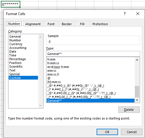
To repeat a specific character in your custom Excel format so that it fills the column width, type an asterisk (*) before the character.
For example, to include enough equality signs after a number to fill the cell, use this number format: #*=
Or, you can include leading zeros by adding *0 before any number format, e.g. *0# 
This formatting technique is commonly used to change cell alignment as demonstrated in the next formatting tip.
How to change alignment in Excel with custom number format
A usual way to change alignment in Excel is using the Alignment tab on the ribbon. However, you can «hardcode» cell alignment in a custom number format if needed.
For example, to align numbers left in a cell, type an asterisk and a space after the number code, for example: «#,###* » (double quotes are used only to show that an asterisk is followed by a space, you don’t need them in a real format code).
Making a step further, you could have numbers aligned left and text entries aligned right using this custom format:
#,###* ; -#,###* ; 0* ;* @ 
This method is used in the built-in Excel Accounting format . If you apply the Accounting format to some cell, then open the Format Cells dialog, switch to the Custom category and look at the Type box, you will see this format code:
The asterisk that follows the currency sign tells Excel to repeat the subsequent space character until the width of a cell is filled. This is why the Accounting number format aligns the currency symbol to the left, number to the right, and adds as many spaces as necessary in between.
Apply custom number formats based on conditions
To have your custom Excel format applied only if a number meets a certain condition, type the condition consisting of a comparison operator and a value, and enclose it in square brackets [].
For example, to displays numbers that are less than 10 in a red font color, and numbers that are greater than or equal to 10 in a green color, use this format code:
Additionally, you can specify the desired number format, e.g. show 2 decimal places:
[Red][ =10]0.00 
And here is another extremely useful, though rarely used formatting tip. If a cell displays both numbers and text, you can make a conditional format to show a noun in a singular or plural form depending on the number. For example:
The above format code works as follows:
- If a cell value is equal to 1, it will display as «1 mile«.
- If a cell value is greater than 1, the plural form «miles» will show up. Say, the number 3.5 will display as «3.5 miles«.
Taking the example further, you can display fractions instead of decimals:
In this case, the value 3.5 will appear as «3 1/2 miles«. 
Tip. To apply more sophisticated conditions, use Excel’s Conditional Formatting feature, which is specially designed to handle the task.
Dates and times formats in Excel
Excel date and times formats are a very specific case, and they have their own format codes. For the detailed information and examples, please check out the following tutorials:
Well, this is how you can change number format in Excel and create your own formatting. Finally, here’s a couple of tips to quickly apply your custom formats to other cells and workbooks:
- A custom Excel format is stored in the workbook in which it is created and is not available in any other workbook. To use a custom format in a new workbook, you can save the current file as a template, and then use it as the basis for a new workbook.
- To apply a custom format to other cells in a click, save it as an Excel style — just select any cell with the required format, go to the Home tab >Styles group, and click New Cell Style….
To explore the formatting tips further, you can download a copy of the Excel Custom Number Format workbook we used in this tutorial. I thank you for reading and hope to see you again next week!
Источник
In this article, we will learn How to custom format cell in Excel.
What is the Format cell option ?
Custom format option lets you change the format of the number inside the cell. This is required because excel reads date and Time as General numbers. Format cell option allows you to change in any of the given formats.
- General
- Number
- Currency
- Accounting
- Date
- Time
- Percentage
- Fraction
- Scientific
- Text
- Special
- Custom
Under the custom option you can use the type of format required.
You can access the Format cell option in the Home tab to change the format as shown below.
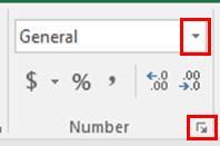
Just drop down from arrow and select from the view option or click the right most red box button as shown in the above image to open More number formats
There are some shortcuts to convert a number into different formats.
| Format | Shortcut key |
| General number | Ctrl + Shift + ~ |
| Currency format | Ctrl Shift $ |
| Percentage format | Ctrl Shift % |
| Scientific format | Ctrl + Shift + ^ |
| Date format | Ctrl + Shift + # |
| Time format | Ctrl + Shift + @ |
| Custom formats | Ctrl + 1 |
Example :
All of these might be confusing to understand. Let’s understand how to use the function using an example. Here we will see how one number can be seen many different formats.
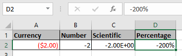
These are some of the format options of the number -2 in different formats.
Now there’s one more thing. Numbers represent so many values in a text as Date, Time and currency. So Sometimes you need to change the format cell type to required field type using Format cell option.

Use the format cell option shown below or Ctrl + 1 shortcut keyboard key that will open a full Format cell dialog box

Changing the format you will get
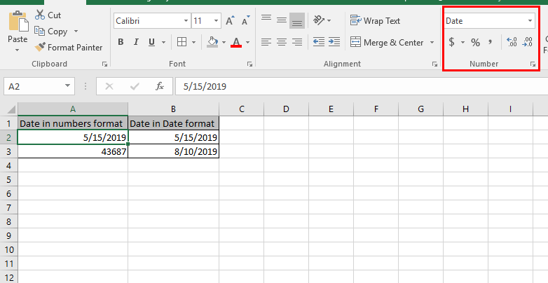
As you can see from the above snapshot that the number in general representation is converted to date format.
Here are all the observational notes using the custom format option in Excel
Notes :
- Use number formatting to convert the value into another format. The value remains the same.
- Use percentage format when using percentage rate values in Excel.
- Formula starts with ( = ) sign.
- Sometimes there exist a curly braces in the start of formula, which is an array formula and called using the Ctrl + Shift + Enter. Do not put curly braces manually.
- Text values and characters are always given using quotes or using cell reference
- Numerical values can be given directly or using the cell reference.
- Array can be given using the array reference or using named ranges.
Hope this article about How to custom format cell in Excel is explanatory. Find more articles on calculating values and related Excel formulas here. If you liked our blogs, share it with your friends on Facebook. And also you can follow us on Twitter and Facebook. We would love to hear from you, do let us know how we can improve, complement or innovate our work and make it better for you. Write to us at info@exceltip.com.
Related Articles :
How to use the Shortcut To Toggle Between Absolute and Relative References in Excel : F4 shortcut to convert absolute to relative reference and same shortcut use for vice versa in Excel.
How to use Shortcut Keys for Merge and Center in Excel : Use Alt and then follow h, m and c to Merge and centre cells in Excel.
How to Select Entire Column and Row Using Keyboard Shortcuts in Excel : Use Ctrl + Space to select whole column and Shift + Space to select whole row using keyboard shortcut in Excel
Paste Special Shortcut in Mac and Windows : In windows, the keyboard shortcut for paste special is Ctrl + Alt + V. Whereas in Mac, use Ctrl + COMMAND + V key combination to open the paste special dialog in Excel.
How to Insert Row Shortcut in Excel : Use Ctrl + Shift + = to open the Insert dialog box where you can insert row, column or cells in Excel.
50 Excel Shortcuts to Increase Your Productivity : Get faster at your tasks in Excel. These shortcuts will help you increase your work efficiency in Excel.
Excel REPLACE vs SUBSTITUTE function: The REPLACE and SUBSTITUTE functions are the most misunderstood functions. To find and replace a given text we use the SUBSTITUTE function. Where REPLACE is used to replace a number of characters in string…
Popular Articles :
How to use the IF Function in Excel : The IF statement in Excel checks the condition and returns a specific value if the condition is TRUE or returns another specific value if FALSE.
How to use the VLOOKUP Function in Excel : This is one of the most used and popular functions of excel that is used to lookup value from different ranges and sheets.
How to use the SUMIF Function in Excel : This is another dashboard essential function. This helps you sum up values on specific conditions.
How to use the COUNTIF Function in Excel : Count values with conditions using this amazing function. You don’t need to filter your data to count specific values. Countif function is essential to prepare your dashboard.
The other day I had to make an excel sheet for tracking all errors across one of the applications we are doing for our customer. The format was something like this,
![]()
We wanted to use a consistent message id format [4 digits: 0001, 0002, … , 1000 etc.]. Now I do not want to type “0001” in excel, instead I wanted to type 1 and I want excel to convert that to 0001 for me. So I started looking for a custom cell format and dug a little deeper to understand those. I thought it would be nice to share them to you all.
First take a look at how the cell formatting dialog box – number tab looks like:

Now apart from the built in types General (leave excel to guess the data format), number, currency, accounting (uses the separators, () notation etc.), date, time, percentage, fraction, scientific, text there are 2 interesting types of formating.
Special: Used for phone number, zipcode, social security number formats depending on the locale you select. For eg. for US they would be phone number [xxx-xxx-xxxx], ssn [xxx-xx-xxxx], zipcode[xxxxx, xxxxx-xxxx].
Custom: Used for creating your own cell formatting structure. This is a bit like regular expressions but in entire microsoftish way. Any cell custom format code will be divided in to 4 parts : positive numbers ; negative numbers ; zeros ; text. If your formatting codes have less number of parts (say 1 or 2 or 3) excel will use some common sense to find out which ones are for what.
Ok, without further confusion, this is probably how you can use the custom cell formatting feature in Microsoft excel.

Some explanation that you can skip if you already get it
- For formatting a number [eg. 1] to fixed number of digits [eg. 0001] you have to use 0000 as the custom formatting code
- For formatting a phone number [eg. 18003333333] to a standard phone number format [eg. 1 800-333-3333] you have to use 0 000-000-0000 as the custom formatting code
- To fill rest of the cell with a character of your choice [eg. *] you have to use @**(this applies for text inputs)
What are your favorite data formatting tricks? [Also read : Creating cool dashboards in excel using conditional cell formatting]
Share this tip with your colleagues

Get FREE Excel + Power BI Tips
Simple, fun and useful emails, once per week.
Learn & be awesome.
-
212 Comments -
Ask a question or say something… -
Tagged under
cell, formatting, hacks, how to, information, Learn Excel, microsoft, spreadsheet, technology, tips, tricks
-
Category:
Charts and Graphs, Featured, hacks, Learn Excel

Welcome to Chandoo.org
Thank you so much for visiting. My aim is to make you awesome in Excel & Power BI. I do this by sharing videos, tips, examples and downloads on this website. There are more than 1,000 pages with all things Excel, Power BI, Dashboards & VBA here. Go ahead and spend few minutes to be AWESOME.
Read my story • FREE Excel tips book


Excel School made me great at work.
5/5

From simple to complex, there is a formula for every occasion. Check out the list now.

Calendars, invoices, trackers and much more. All free, fun and fantastic.

Power Query, Data model, DAX, Filters, Slicers, Conditional formats and beautiful charts. It’s all here.

Still on fence about Power BI? In this getting started guide, learn what is Power BI, how to get it and how to create your first report from scratch.

- Excel for beginners
- Advanced Excel Skills
- Excel Dashboards
- Complete guide to Pivot Tables
- Top 10 Excel Formulas
- Excel Shortcuts
- #Awesome Budget vs. Actual Chart
- 40+ VBA Examples
Related Tips
212 Responses to “Custom Cell Formatting in Excel – Few Tips & Tricks”
-
[…] Krunker | Technology Around the World wrote an interesting post today onHere’s a quick excerpt The other day I had to make an excel sheet for tracking all errors across one of the applications we are doing for our customer. The format was something like this, We wanted to use a consistent message id format [4 digits: 0001, 0002, … , 1000 etc.]. Now I do not want to type “0001? in excel, instead I wanted to type 1 and I want excel to convert that to 0001 for me. So I started looking for a custom cell format and dug a little deeper to understand those. I thought it would be nice to shar […]
-
 Swati says:
 Many Thanks. This is really informative. I want to know how a program can read»contents» of a Custom cell. WRT the eg. above, if the Value After is 0001, when a program reads the value, it reads it as 1 instead of 0001.
-
@Swati — you are welcome. Yeah, you are right, the cell format changes the value at UI level alone, when you access the value from formulas / vba / scripts the value is still what you have entered (ie 1 in your case)
Welcome to PHD, enjoy 🙂
-
Swati says:
Thanks. So in case, I want my program to pick the value the way it appears on the UI, how can that be done?
-
@Swati … wow, thats a tricky one.
You can use the following function:
Function fetchValue(incell As Range) As String
fetchValue = incell.Text
End FunctionJust add it to your workbook’s VBA code in a module and start accessing it from code. I havent tested it extensively, but it seem to be working fine.
Just curious, why would you need the value of the cell as it is formatted against its actual value in code? Chalo, let me know if this is working for you 🙂
-
Ahtesham says:
I HAVE USED CUSTOM FORMATTING AND ADDED PREFIX AND SUFFIX TO A NUMBER IN WHOLE ROW. BUT NOW WHEN I COPY IT, IT SHOWS THE ORIGINAL NOT THE FORMATTED NUMBER. KINDLY HELP.
-
-
I found your blog via Google while searching for free personal finance tips and your post regarding use custom cell formats in Microsoft Excel — tips | Pointy Haired Dilbert — Chandoo.org looks very interesting to me. I always enjoy coming to this site because you offer great tips and advice for people like me who can always use a few good pointers. I will be getting my friends to pop around fairly soon.
-
[…] read Using Custom Cell Formats in Excel — Tips & Tricks to findout how to format dates, currencies, special formats etc. Tags: excel, formatting, howto, […]
-
JITENDER says:
Dear Sir,
I also have some problem in excel, can you solve my problem. I gave you my email ID .Thanking you
-
sandeep says:
I want to sort/filter data by their different custom format is it possible to do so. ex.
5.660/Pcs
0.258/Sqm
5.213/Rmts
5/nosthese kind of custom formatted details are downloaded from Tally ERP -9 I want to sort data by Sqm/Pcs/Rmts and other UOM . all data are in custom number format
-
-
@Jitender … surething, you are welcome to write a comment explaining the problem, that way, even if I dont know the solution, there will be one of our excellent readers who would know how to solve it for you, and they may come forward and post it in replies. Otherwise, feel free to write me an email… 🙂
-
kc says:
I’ve been browsing this thread for awhile and there is one format I can’t seem to create a custom format for. If I want to go from 1234-5678 to 12345678 how can I do that?
Thanks! -
@ Kc… thanks,
I dont know any format that can 12345678 from 1234-5678, you can use substitute(«-«,»»,1234-5678) though… let me know if you findout how to do this.. I will sponsor you a donut 2.0 😀
-
[…] thus making the 01001 as 1001. Worry not, you can use rept() the extra needed zeros. You can also custom format cell contents to display zip codes, phone numbers, ssn etc. Example: Use zipcode & REPT(«0»,5-LEN(zipcode)) to convert zipcode 1001 to […]
-
[…] Try these other date formats as well. Learn more about custom cell formatting. […]
-
[…] How to use custom cell formats in Microsoft Excel — tips | Pointy Haired Dilbert — Chandoo.org Custom Cell Formatting in Excel — Few Tips & Tricks […]
-
asghar says:
i want to calculate formula for example: 500PCS X 12 = 6000. but when i mention PCS or doz or set after any digit as above, formula says #VALUE. It can not give result.
suppose 500PCS IN A CELL x 12 IS IN B CELL FORMULA IS =SUM(A1*B1). kindly help me abt.-
@Asghar: Welcome to Chandoo.org.
You can correct the formula in the following ways:
(Simple) do not enter PCS, Doz etc in the cell A1, but use another cell like A2 maintain the units.
(slightly complex) use custom formats to display «PCS» or «Doz» next to the value so that formulas still work while you can maintain the desired look. You can do this by defining a custom formatting code like 0 «PCS» or 0 «doz»See this image.
Let us know if you still have any trouble. 🙂
-
AnnaK says:
Asghar, I have another way to fix your solution
Select the cells you want to put the number, Go to Number formatting/ Customer and type ####»PCS»
This will add PCS to the cells you choose, you just only type 500 or any number you want. Then do your calculations, hope that helps. Now choose the easiest way you want
-
-
Somnath says:
Asghar,
You can try using the left function. Using your example:
=(LEFT(A1,3)*B1) ought to give you 6000.Thus said, you need to customize this formula in case the number of units run into thousands. 🙂
-
Somnath says:
Chandoo,
I am enjoying my first visit to your site. Looking at the thread posted by KC, you are absolutely right. Substitute function is the way to go about it.Considering 1234-5678 is in cell A1, the substitute function will be:
=SUBSTITUTE(A1,»-«,»»,1)Lots of good stuff in here!!! Makes me feel nostalgic about my good old college days. 🙂
-
@Somnath: thank you, I am very happy you liked the site and actively contributing to it. I have learned so much from readers like you and I really enjoy interacting with new people through this site. Keep visiting and share your knowledge with all of us. 🙂
-
HOW ABOUT THIS …12345-12 => 12345-13 ( THE LAST DIGIT )
12345-19=> 12345-20 ( PO WITH RUNNING NO.)
Any tips.
-
Suril says:
@Din: Assuming the value 12345-12 is in cell A1, using the formula =LEFT(A1,6)&RIGHT(A1,2)+1 will give you the desired result. A more refined formula is =LEFT(A1,SEARCH(«-«,A1,1))&RIGHT(A1,LEN(A1)-SEARCH(«-«,A1,1))+1 which will work will any number of digits.
-
Suril says:
assuming the value to be changed is in cell A1, ‘=LEFT(A1,SEARCH(«-«,A1,1))&RIGHT(A1,LEN(A1)-SEARCH(«-«,A1,1))+1’ should work:-)
-
2581-14 #NAME? A1, ‘=LEFT(A1,SEARCH(“-”,A1,1))&RIGHT(A1,LEN(A1)-SEARCH(“-”,A1,1))+1
I TRY RESULT SHOWN . CAN YOU HELP !
-
-
-
-
James says:
I have a problem when formatting a cell that has 16 or more digits, using the Custom format. We are working with Credit Card numbers and want to be able to enter them as a 16 digit number like this: 1234123412341234 but want them to look like this: 1234 1234 1234 1234
The problem we’re having is that the last digit always turns into a 0 (zero) and the number ends up looking like this: 1234 1234 1234 1230
The custom format type we created is: 0000 0000 0000 0000 but we’ve also tried: #### #### #### #### with the same results.
This only happens when using 16 or more digits. If we use 15 or less digits, the Custom format works fine. Unfortunately, credit cards have 16 digits so we’re stuck with the problem.
We’ve tried this on Excel 2007 with service pack 1 and on Excel 2000 with service pack 3 with the same results. The Operating Systems we’ve tried it on are Windows XP with Service Pack 3 (and all other Microsoft Updates installed) and on Windows 2000 with Service Pack 4.
Any help would be greatly appreciated. -
[…] asks in Custom Cell Formatting in Excel Post, I have a problem when formatting a cell that has 16 or more digits … We are working […]
-
SReid says:
Hi Chandoo —
Awesome suggestions…. big question for ya! We have P.O. numbers that come from a system with the standard format of XX-XXXXX. The first 2 XX are the year — the very last X could be there or not be there depending on whether we are at the beginning of the year or the end of the year. When we dump data from this system into excel, 95% of the PO numbers format correctly in the column: 09-1234 or 09-12345 for example.The other 5% show as a date in the field: Sep-67. If you place your cursor in the formula bar it says 9/1/8267. The REAL PO number for that one is 09-8267. I’ve tried a ton of different ways to try and make a custom format for the user and am coming up blank every time.
Any help would be of tremendous help! Thanks!
SReid-
@SReid: welcome to PHD. I will try this and get back to you. But I guess the custom code 00″-«00000 should work?
-
-
SReid says:
Hi Chandoo — Sorry no luck on that format. The correct PO number is 08-8979. When dumped into Excel, and reviewing it the cell — it changed to a date format of Aug-79. If looking at it in the formula bar, it is 8/1/8979. If I apply the custom format you suggested, it changes the PO number in the cell to 25-85766 and in the formula bar to 2585766 (without the dash). Crazy I tell you! Crazy!
Thanks! SReid
-
@SReid: when you dump data, excel assumes the formats of the data it is pasting. so even before pasting the data, you need to set the cell formats. Also, I see that your data comes with hyphen (-), in which case, you need not use any format codes, but just set the cell formats to TEXT from GENERAL. If you paste a lot of data, select the entire sheet and press ctrl+1 and set the formats to text.
Let me know if you have some problems
-
cybpsych says:
hi chandoo,
hope you can help me with this problem; it’s something about number formatting and «Creating dash boards using excel conditional formatting» @ http://snipurl.com/g2rwb
consider these data:
set 1: 2851/3.00 = 0.001052262…… = 0.11% (% with 2 decimal)
set 2: 2851/3.01 = 0.00105576….. = 0.11% (% with 2 decimal)when i do a IF comparison for both 0.11%, it’s NOT EQUAL. This creates a little problem with the dashboard formula whereby it will show icon ? instead of ?.
The only way to ‘solve’ this is to force format each cell with this: =text(2851/3.00,»0.00%») and =text(2851/3.01,»0.00%»). Only then that bot sets are EQUAL.
As there a simpler way to TRULY HARD FIX the decimal numbers in a percentage format? 0.11% == 0.11% 🙂
Thanks!
-
cybpsych says:
rewrite:
This creates a little problem with the dashboard formula whereby it will show icon «^» instead of «o».
-
cybpsych,
use ROUND(2851/3.00,4) and ROUND(2851/3.01,4) instead and the two values will be equal.
-
SReid says:
Hi CHandoo….
I am dumping the data from SQL. It is a varchar field. I have tried setting the column to TEXT. This does not work. SQL has the field (correctly) as 08-8979. When dumped to Excel, it changes it to: Aug-79. If I try to change the format to TEXT, the data then CHANGES to: 25-85766.The crazy part of this is that it only happens on about 5% of the data in that column. All of the rest of the data comes over in the correct XX-XXXXX format.
Any other ideas?
Thanks!
-
@SReid: Hmm… do you have some automated program that is dumping the data from SQL? What do you mean when you say you have set the column to text? Is it in excel or sql. You should set it in excel. Another thing that comes to my mind is to use text import wizard and select the column type as text in the wizard. I know this could take more time, but if you import once in a blue moon it might be worth the effort.
In the worst case, you may need to get some vba that would take the sql data and properly dump it.
-
Also, when I try to paste the value 08-8979 in to excel, even though cell format is «TEXT» it is still displayed as Aug-79, but when I select the little paste icon beneath the pasted cell and say «match destination format» it is correctly displayed as 08-8979. May be excel is forcing itself to use source formatting (weird how it decided that source format is in date…?).
-
LINDSEY says:
I know this was posted 3 years ago but maybe someone else will have a similar issue so here is the answer: I’m not sure why exactly but if you use 00″-«0000 it works. When you put in the 5th 0 it changes it to 00-88979? Strange! But it worked. 🙂
-
-
-
-
cybpsych says:
hi chandoo, i’m curious on the following:
how to custom format this number: 883509615 —> 883.509615 Million or 0.883509615 Billion?
don’t bother on the decimal numbers; I can round them up as per Robert’s suggestion above 😉
thanks!
-
@Cybpsych: hmm, I am not aware of custom format codes that can do this. I can suggest a formula version though, but I guess it should be obvious. Let me know if you come across any custom codes that can do this. btw, if you use the numbers in charts, excel has a facility to show them in millions, billions etc. but when they are used in cells… I am not sure which option would convert them to million etc. at format level while keeping the value intact…
-
-
cybpsych,
use the thousand operator in custom number format:
Assumed you have the cell value 12345678.
Custom format #,###.00, will display 12,345.68
Custom format #,###.00,, will display 12.35
Custom format #,###.00,,, will display 0.01-
Ramesh says:
this format is very good but my problem is not resolved i am entering cell s value is 1,10,000 this value covet to 1.10 Plz help and send me the anwer to my id
-
-
cybpsych says:
thanks robert for your help 😉
-
JohnM says:
Hey Chandoo,
I’ve tried relentlessly to figure this one out, but I’ve given up at this point. I have a sheet full of millions of entries that I input onto a worksheet, which are then pulled into a more intricate report using vlookup. Within one of the columns is a UPC code that i’m trying to transfer, and it should contain 12 digits (000000000000 custom number format). I have changed the columns format to suit that, so that some of the columns that had 11 digits will now have 12. However, even though I have changed the format, the 11 digit numbers remain unchanged until i open the formula cell and click into another cell. I obviously can not do this to the 100’s of entries every week….do you have any suggestions?! thanks!
-
@Robert: Very cool tip, I didnt know we can do that…
@JohnM: Welcome to PHD. I have tried to replicate your problem in excel by entering dummy values in 10000 odd rows. The values had a mix of 11 digits and 12 digits among them. But when format them using the custom format code 000000000000, they are instantly changed. So I assume it should work the same way for you. May be because there are a million values, excel is choking under the pressure and not running the formats until someone navigates to the cell. But I would imagine the formats working perfectly if you ever need to print them.
-
cybpsych says:
hi chandoo/john,
i believe this is happening because the data is imported from other sources?
if so, Excel doesn’t treat the «numbers» as numbers. You will need to convert them into proper numbers in Excel.
If AutoCorrect is on, select the range and hover aroudn the GREEN corner arrow. Select the «Covert to Number».
-
[…] to the data label. It is one of my favorite tricks in excel and I have written about it in introduction to custom cell formatting in excel, number formatting in excel using custom codes, showing decimal values only when needed […]
-
[…] when you do this, you need to enable wrap-text feature for that cell from cell formatting dailog (ctrl+1) to ensure proper […]
-
[…] lines in a cell | Learn Excel | Pointy Haired Dilbert: Charting & Excel Tips — Chandoo.org on Custom Cell Formatting in Excel — Few Tips & TricksHow to Get Colors in Excel Chart Data Lables — Formatting Trick | Charts & Graphs | Pointy […]
-
[…] use the custom cell formatting (more here) code […]
-
Wes Gibbs says:
If I wanted all cells within column A to only have 7 digit numbers how can this be done? If a user wanted to enter 12, that 12 would be converted to: 0000012. I basically only want values: 0, 1, 2, 3, 4, 5, 6, 7, 8, and 9 and locations 1, 2, 3, 4, 5, 6, and 7 of the 7 digit string. I’ve been fooling with some time with no lock. I first converted the entire column A to text and gave it a format of 0000000 so that it got preceding zeros when values that are less than 7 digits are given. Then I started fooling with the Data Validaion putting: =LEN($A$1)=7
but it doesn’t seem to work quite right.
-
Messam says:
Hello !! I am facing a problem in displaying value in this format «1/1» (Without inverted commas).
Currently I have information in this form 1 / 1. When I remove spaces from the cell, the value is automatically converted to Date Format as 1-Jan. Can anyone of you help me getting the required format after removing spaces.
Many Thanks in advance !
-
Messam says:
Making the problem more clear !
Current Value of the cell: 1 / 1
After removal of space from the cell
New Value of the cell: 1-Jan
Required Format: 1/1 (without space)
An urgent response will be highly appreciated !! Thanks !!
-
Aires says:
@Messam there’s a method that comes from Lotus 1-2-3. When you’re typing the value, start with a ‘ (apostrophe). So, in your example, typing ‘1/1 should work properly.
Hope that helps.
-
Messam says:
Many Thanks !!
I got a solution myself as well.
The same can be done using a function in excel called «SUBSTITUTE».
-
Messam says:
Aires: I could not understand the solution you provided. Can you please explain?!?!
-
@Messam.. you can also force excel to consider a cell’s contents as text by setting the formatting type to «text» from «general» this will leave 1/1 as 1/1 instead of making it jan-1
-
[…] and “n”, user should type “1″ and “0″. Then we can use custom number formatting to conditionally display the tick mark […]
-
Elisha says:
re: John M
I am having the exact same problem as you! Did anyone ever find a solution??
-
Elisha says:
I had tried everything I could think of for the problem John described that I was also having.
I had this issue with phone numbers and zip codes.
I decided to use text to columns to split up my zip+4 column and accidentally clicked finish on the first step (with delimited selected) and magically my entire column of data updated to display the correct format. I repeated my «mistake» on the phone number column, which was also not updating to the correct format, and it worked there too!
It’s a silly way to have to do it, but hey, whatever works…!
I would love to know what is causing this issue though. -
@Elisha… welcome to PHD and thanks for your comments.
Did you try using the TEXT formula. It forces the formats by changing the values to text. For eg. =text(a1,»00000-0000″) would force the value A1 to appear as zip+4 format.
-
Kim says:
I have a spreadsheet of X’s and I want to add the number of Xs in each column. I’d like to custom fomat X so that it reads as 1 and then I can add all the 1s. How would I do that?
-
JAY says:
Hi chandoo
i want to convert to figures to text . how can do it
it means 5000/- :- Five Thousand Only. -
Prashant says:
Hi chandoo
Custom Cell Formatting in Excel-
Select column — RAM CHANDRA
Value before- RAM CHANDRA
Costume Format- «MR.» @
Value After- MR. RAM CHANDRA -
Jay says:
Hi
chanduI want to no. tricks but in below this format
****12,345.00 this format .
please send me some tricks for this format -
Hui… says:
Jay, try
«****»#,###.00 -
[…] custom number format […]
-
plz help me says:
dear sir.
i have two problems that are :1) in a work sheet, list of names, automatically added the email domain [eg: snarif @honda.com,munni@honda.com; tazman@honda.com]
2) few numbers are available, i want those numbers in words [5000 will show Five thousand, 100 will show One Hundrate] -
jay says:
hi chandoo
make a telephone directory in excel using visual basic and create the derectory
please give me idia’s -
Leo says:
Dear Chandoo,
I want to display codes of 5 digits, but sometimes it has 3 decimal places after those 5 digits. I don’t want to show the decimal unless it is followed by the 3 decimal places. If I use ?????.??? or #####.### it always shows the decimal after the 5 digit numbers without any decimals following them. For example 12345 would show up as 12345., and 12345.678 would show as that. The latter is fine, but the first example needs to drop the decimal point. Any ideas will be appreciated. Thank you. -
Ensav says:
Dear Chandoo,
I used the following custom format (found in a forum) to display a hyphen instead of zero… But the problem is that after changing to this, I can not align the content to center or left.
_(* #,##0_);_(* (#,##0);_(* «-«_);_(@_). Could you please check and advise. Thanks -
Hui… says:
@Ensav
try
_(* #,##0_);_(* (#,##0);_( -_);_(@_)
No need for the quotes around the — unless you want them -
Ensav says:
I tried. It works only with the cells of ‘zero’ values and not with the remaining cells having other values. Normally the format applies to all sheets / area. Any other way…. Thanks
-
Fortunate says:
Hi Chandu,
I need to format the values as follows and have no idea how to do it.
00:17:42 —> 00d 17h 42m
Please help.
-
@Fortunate
Use the Custon Number Format
Ctrl 1, Custom
d»d» [h]»h» mm»m»
Make sure all the «‘s are «, retype if necessary -
Fortunate says:
Hi Hui…,
Thanks for your quick reply..
It is not working 🙁 It is giving the same output 00:17:42I think we need something to remove the colons. Please help!
-
ltg says:
Someone asked me about this today…
Enter 1-2 and have it convert to 1′-02″. 1-10 goes to 1′-10″, etc. Actually, it might be more important to have 1-6 convert to 1.5, 1-2 convert to 2.1666667, etc because what it really needs to do is multiply/add correctly. So maybe the solution is not so much in the formatting, as much as it is in the formula? I guess the user could use TEXT for input so it would stay as 1-10, then have the formula parse the «-«, and convert it to 1 + xx/12? Or any better ideas?
-
amol says:
send me excel notes
-
Sam says:
Thanks for this great tip, was really helpful
-
Raj Kiran says:
Hi Chandoo,
I have always been a frequent visitor and reader of your posts. Inspired by the same, I have done a project performance dashboard for my organization.
Currently am revisiting the dashboard to be more dynamic. In the process I am facing a slight problem. I am trying extract data from the database to a single cell using vlookup. Now the data is of different types like dates, percentages, numbers and text. But I am unable to make the cell receiving these data to have multiple formats. Can you please suggest on how to make a cell recieve different data types.
This will be of real great help.
Thank you in advance
Raj Kiran -
naveen says:
Hi chandu,
this is my first visit to your site. Can you tell me that if I have the data with comma as seperators and decimal 2 places , how to convert it to general format. -
Lisa says:
Hello all and please help!
One unit is six minutes which I need to display as 00:06. Ten units is one hour which needs to be displayed as 01:00 and so on.
Then there is an hourly rate, say £60 per hour. The final column needs to show the total amount.
How do I show the time in minutes but multiply by the number of units??
TIA
Lisa -
@Lisa
If cell F1 has your units
In G1 put =F1*(6/(24*60))
Apply Custom Format as hh:mm
in H1 =F1*60
Apply £ format to H1 -
Brian says:
Is there a way to have a cell value always show a «+» if it is a positive number, and an «-» if the value is negative?
Example: 0.6% would show as +0.6%.
-0.8% would show as is.-
venu says:
Brian,
Ctrl+1
Choose Custom
Type +0:-0
That will do the trick
-
-
Sam says:
Hi..
I was trying to format numbers in the Indian format of Lakhs & crores..
I went to custom and typed the following 00,00,000
But excel keeps showing the default of millions & billions 000,000,000
Pls help
-
Sam says:
Dear Naveen (#65),
you can try this shortcut Ctrl+Shift+~
-
zemane says:
On the -12 and 12 example, where did the Rs. came from?
-
Roopa says:
Hi,
I am trying to custom format a particular cell in excel to display the figure in lakhs
Original number is 11111111. This should convert to 111 lakhs and the cell value should be shown as 111
Can you please let me know if it is possible in custom format. I tried
0″.»0,, which returns in crores (1.1) and 0″.»0, which returns 1111-
@Roopa
It is only possible to divide numbers by 10^3, 10^6, 10^9 etc
This is done by adding a comma to the custom format code
so
123456 displayed as «#,.000» will display 123.456
123456789 displayed as «#,,.000» will display 123.457
.
The only other small modification you could use is to use a helper cell with
=TEXT(10*B4,»0,,»)
so that 11111111
will display as 111, except that internally it will hold 111111110-
Roopa says:
Hi Hui,
Thanks for your quick reply although I do have to admit that the solution cannot be adopted since this particular cell is only a format template cell and does not accept any links or formulas. Also the internal value of the cell cannot change since the same base has to be used for all the conversions( thousands, millions, crores etc)
I needed some expert confirmation before calling quits 🙂Thanks a lot
Roopa
-
-
@Roopa
Thanx to Kyle below, You can use a Custom Format of
#,,," Lakhs" %%
To display what you want
Use the above Custom Format and insert a Ctrl J before the first %
Then set your cell to word wrap and top/centre alignment
-
-
A.Mac says:
Hello,
I’m wondering if there is a way to have Excel display a value 1000 times greater than its actual value using custom number formats.
For example, if I give a cell the value 0.00943 how can I get it to display as 9.43 mA, but still have the value 0.00943 V so I can perform other operations on it. I realize that I can simply multiply the cell value by 1000, but then if I want to use that value in another calculation I need to divide by 1000 to get it back to its original value
-
Kyle McGhee says:
Hi A.Mac,
Select the cells you want to format and enter this in the custom format:
.# «mA»%%before you press enter, put the cursor between the » and the % and press ctrl+j which will insert a carriage return.
And then on the Alignment tab of the Format Cells dialog, select word wrap. .000943 becomes 94.3 mA.
The rows have to be normal height, if they are larger you will see the two %% symbols. Change the number of # after the decimal if you want to increase/decrease the number of digits after the decimal
Kyle
-
Kyle McGhee says:
sorry just realized that mine was 10,000 and gave 94.3 and you wanted 9.43, so same deal except
.##, «mA»%%% — this is multiplying by 1,000,000 with the three % and also dividing by 1,000 with the commaplus the ctrl+j between » and % and word wrap will give 9.43
-
-
Neat trick Kyle
But to get from 0.00943 to 9.43 mA you need the following format
0.#, "mA"%%%
The , divides it my 1000 and the 3 %’s multiply by 100 eachAlso the cell needs to be Top Aligned as well as have word wrap
-
Kyle McGhee says:
Thanks Hui. I noticed that, as you can probably see now. Are you sure about the top alignment? I just tried it with all vertical and horizontal alignment combinations and the %% symbols stayed out of sight. Row height is the 15 (20 pixels).
-
-
A.Mac says:
Thanks for your help gentlemen.
It’s too bad there wasn’t a more elegant solution, but that did the trick.
-
-
Wayne says:
How to use my own text wording in a cell from the results from another cell in excel 2010. Example When H17 is a negative dollar value I would like the word in E17 to read Disqualified in the colour red. When H17 is a positive dollar value I would like to have the word in E17 to read QUALIFIED in the colour blue.
Thank you -
[…] thanks to a tip I picked up from Kyle who responded to a post here at Chandoo.org they are all […]
-
Veena says:
Hi Chandoo,
I have a scenraio here, where the cell needs to hold leading zero’s for example Cell A1 will have the 0123456, cells A2 can have the data as 0012345, Cell A3 can have the data as 1234567.
I am unable to fix this issue with custome format. Can this issue be fixed with custom format.
Thank You.
-
venu says:
Hi Veena,
In Custom format type zero seven times i.e. 0000000
It worked for me
-
-
[…] in the new box, and towards the bottom are some more time formats to choose from. There are some tips here on how to use the custom […]
-
Amit Gogna says:
Hi,
I too am stuck with a peculiar issue.
I have a sheet with seconds (from 0 to 10,000) against each person stating how much they used the phone on each day, I have converted the seconds to time by using <>, where c2 is the cell (column) for seconds. I wanted to display this as <>. So I tried using the custom formatting of the cell by putting <>. Worked fine till the usage goes over 30 days. If the person uses the phone for (lets say) 35 days, 2 hours and 31 minutes, it displays <>. Is there ant setting to get the absolute number of days stated?
Thanks.
-
Scott says:
Chandoo,
I am trying to custom format a cell in Microsoft Excel. I want to set up a custom format that will add a specified % to any number I input into a cell. What type of format/formula must be included for this to work?…………
Thanks-
@Scott
any code just add an % to the end
eg:
#.00%
0.0%
etc-
Scott says:
I did not explain myself well. Sorry.
I want to add 2% to any number I input into the cell by using a custom format.
For example in the cell: when I input 3, I want the cell to multiply it by 2%, giving me the output of 3.06.
I am not sure this is even possible.
Thank you.
Scott-
@Scott
As you suspected, Excel can’t do that with Custom Formatting
You can do it to a cell using VBA if required.
-
-
-
-
Debbie M says:
Thank you for your help!! 🙂
Can you format cells to always have a negative number no matter what you type in. I need like 15 cells in one column and 35 cells in another column?
Thank you!
Debbie-
@Debbie
Just put a negative sign in front of your favorite Custom Format style
eg:
-#,##0;-#,##0
-
-
Hiren says:
can someone tell me how to write number 1234567 as 1,234,567.00
Thanks
-
Hiren says:
can someone tell me how to write number 1234567 as 1,234,567.00
in Excel 2010
Thanks -
Prasad says:
Hi,
Can anyone help me with the below issue,
I have a report in excel in which all the amounts are in custom format. I wanted to paste the same in Text format. (For e.g. amount in custom format is shown as 100 Dr however when we formula bar we could see only 100; I want 100 Dr to be shownn on formula bar) Could you help me on this.
Thanks,
Prasad-
@Prasad
Custom Formats only change the displayed format of the cells contents in the Cell itself
In your case the cell contains the number 100
but the cell displays it as 100 Dr
The Formula Bar always displays the cells contents wether it is Text, a Value or a Formula
-
-
Kevin says:
Need some help I have a group of numbers that have a letter in it and I am trying to get the format to match but coming up with nothing.
Example: 24A102
This is what I am wanting to get: 24-A1-02
-
@Kevin
Using a helper cell:
=LEFT(A2,2)&"-"&MID(A2,3,2)&"-"&RIGHT(A2,2)
-
-
hello can any one tell me how to use formula for this particular format in custom
Format — first 5 character, then 4 digit, then one character
eg. AAAA12345A
if user doeas not follow above formate error should display.I just want how to put formula
-
HP says:
Hi Chandoo,
I am trying to format the following number in Excel -10 can you tell me how can i do it. Example is below, when i import the data it comes with 1,25M and so on, how can i convert them with 1,250,000 etc.1,25M = 1,250,000
5,00M = 5,000,000-
@HP
Try:
=LEFT(SUBSTITUTE(A1,",",".",1),LEN(A1)-1)*1000000
Then use a Custom number format as #,###,###
-
-
Ravi says:
dear sir
how to split date month ,year time in one word example :20120621121201-
Ravi says:
Actual :2012/06/21 12:12:01
-
You can use this formula to convert that number to a real date/time value…
=1*TEXT(A2,»0000-00-00 00:00:00″)
and then format the cell to display it the way you want. I am guessing you would want this Custom Format type pattern…
yyyy/mm/dd hh:mm:ss
-
Ravi says:
Dear sir
yyyy/mm/dd hh:mm:ss how to apply in excel sheet
-
@Ravi
Select the cells
Ctrl 1 or Right Click, Format Cells
On the Number Tab, select Custom
In the Type: Box type:yyyy/mm/dd hh:mm:ss
Ok
-
-
Ravi says:
Dear sir
Thank you very much for our instant support we happy with solution.
happy week end
Regards
Ravi
-
-
-
-
Cat says:
Hey, i have been having a problem formatting a cell. Since everyone here seems like experts compared to me, i hope you can help me solve this.
In a cell the data is input as «abc00120120101001» where I need it to be formatted into «abc001-20120101-001» and then in a different cell I need «abc001».
Any suggestions would be wonderful. -
MaxiM says:
Chandoo,
Kindly assist how to format/customize the Arrow, the arrow pointing up is color Red while the arrow pointing down is Color Green.
Tnx alot in advance
mxm
-
Lasapa says:
Hi!
Is there a simple way to customise a cell with units that I have specified in another cell (or more)?
e.g.
I have two cells:
A1 — where I specify a unit.
A2 — where I enter a value.I would like cell A2 to have as units the one specified in A1.
So if A1 contains «m» and I enter «25» in A2,
A2 should display «25 m».
(I do not want to use an ‘if’ formulation here because I would like to allow for A1 to take any possible value … It could be ‘Apples’, in which case A2 should display «25 Apples» … etc).Thanks,
LS.-
Lasapa says:
And if possible, I would like to avoid having to define a name for A1 values.
Thanks,
LS. -
Hi LS.. are you still looking for help on this.
Since you just want 25 m or 25 apples for display (but in background the value remains 25, why not readjust the columns so that you enter value first, then pick the unit in next cell. Then you can remove grid lines, adjust alignment so that it looks natural.
-
-
Marg says:
I need to format a cell that would take health card number, sometimes there is a alpha verison code (not always).
Example> 1234 567 890
Example> 1234 567 890 nm or 1234 567 890 ab
I have tried several different ways to custom format a cell but I was unsuccessful.
-
The formatting codes work very well for numbers, not so much for text values like above. So I suggest this:
Select the cell(s) and format them as TEXT.
Now you can enter whatever you want.
When displaying you can easily add a space after 4th and 7th characters like this:
=LEFT(A1,4)&» «&MID(A1,5,3)&» «&MID(A1,8,3)
& IF(LEN(A1)>10,» «&RIGHT(A1,2),»»)
-
-
bilynoz says:
Hello, I received a file with prices in txt format and after opening with Excel 2010 some cells have ‘general’ format and show prices e.g. 114.00 but others have ‘custom’ format and when I click on them, they actually show date in the formula bar, e.g. when I click on price 2.23 it shows 1.2.2023 in the formula bar….I need 2.23 to be the contents of that cell and in a number format, please help!
-
Solomon says:
Hi ,
thanks a lot for your excel formating content. i have a phone field some time it will have 10 digit value (e.g.7877988334) some time it may have phone field with the country code ( e.g. (+91) 7877988334 ). how to create the format to support both of them.
waiting for your reply,
— Solomon -
s9y says:
Hi,
I want to know that how can i force a user to enter this particular number in the sheet. 000-000-000 is the format and number will vary. In addition if there are any alphabets in the entry a typo maybe then they should highlight with some color. Please let me know it its possible.
Thanks in advance.
Sunny-
Suril says:
@Sunny: Assuming that the value is in cell A1.
Go to data — data validation — data validation — allow (custom) and formula should be:
AND(CODE(MID(A1,{1,2,3,4,5,6,7,8,9},1))>=48,CODE(MID(A1,{1,2,3,4,5,6,7,8,9},1))<=57,LEN(A1)=9)
the above formula should be without an «=» sign at the start.
Now under format cells, keep the formatting as 000-000-000. Doing the above will restrict the user from typing anything other than numbers and that too of 9 digits. Now simply copy+paste cell A1 to all the cells wherein this criteria is to be followed. You may delete the data in the cells but the data validation will remain.
Hope this solves it. Let me know.
Regards,
Suril
-
-
TARUN KUMAR says:
hey
I’ve a prblm,
tarunkumar
anilsingh
here are different range names, I want to separate them,
i couldn’t find the way to separate them(text to column is not working in this because it doesn’t have any space,commas,etc.)guys do u have some for this….-
Suril says:
@Tarun, if I understand your question right, you want to tarunkumar to appear as tarun kumar. If so, then there cant be any solution to this! If I got the question wrong then do let me know..
-
-
PO WITH RUNNING NO.
EG 12345- 01( CELL A1 ) . I WANT TO CHANGE B1 TO 12345-02.
ANY FORMULA WITHOUT USING DRAG FILL.
MANY THANKS -
How to set Default character against input character
eg:
I input Vijay but cell shows Mr. Vijay
How to prefix against text-
Suril says:
@vijay you can use «Mr. «@ format under the format cells option.
-
-
YOGESHWAR says:
Hi everyone. Please help with this. I have been tried to find this entirely on Net. Bt i did not fine that.
Actually i have a spreadsheet attched with other sheet.. and i enter value in 1st sheet and its bring the result in 2nd sheet. bt something results are negative number. in cell let say in Cell a1 has some formula and some time result will be change in negative numbers. Once the results automatic change. i want pop-up message instantly. please help me wtih that. Mr. chandoo. please..
Thank you-
Suril says:
@YOGESHWAR
Lets say value you enter is in A1 (Sheet1) and result in A1 (Sheet2). Goto A1 (Sheet1), data — data validation — settings — allow custom and formula should be Sheet2!(A1)<0; goto error message, style — warning and write your warning. Done!-
YOGESHWAR says:
Suril. Thank you very much to reply me back.
actually i have formula in Cell A1 has formula and after entering anything A1 result automatic goes up and down and sometime its in Negative numbers. So once Forumla cells goes in Negative i want to have pop-up error message. instantly.please help me with that.
Thanks again -
YOGESHWAR says:
@ Suril. Dear. i tried with that.. its not working.. its now alowing me to enter any value.on there. please help me with that..
-
Suril says:
can u let me know what error is coming? If you have changed the style to ‘warning’ then only a warming message should be displayed. If you still are unable to enter any value then you may mail me the sheet on suril88@gmail.com.
-
YOGESHWAR says:
Dear Suril. Please accept my invitation that. i just send you on Gtalk.
Thank you very much for you kind help .
-
-
-
-
-
Luke says:
Is there anyway to force a cell to take a certain format and give an error otherwise? I know it can be done in Access, but I can’t figure it out for excell. I have an ID that should be in the format ‘A1234.’ Any ideas?
-
Suril says:
Assuming that the value is in cell A1, you can use the below formula:
=IFERROR(AND(LEN(A1)=5,CODE(MID(A1,{2,3,4,5},2))=0)),»»)You can use the above formula for different formats by modifying it appropriately. To ensure adherance to the format, «validation» should be used.
-
Presto says:
This is truly an awesome site. I have used your thought process(es) to come up with many Excel solutions. I’m stumped on this one, even though it seems simple enough.
I have many rows and columns of data, but for this example, I’ll talk about the first three rows and first two columns. In Column A I have numbers, and in Column B there may or may not be a letter. I am trying to use Custom Format to put the letter (if any) from Column B into Column A (after the number), but have had no success. I realize that since I’m referencing the cell next to it, I’ll probably need to use offset, but perhaps VBA is the only answer. I also have data in Column D/E, F/G, etc. with each series of two columns having a number and then the following column that may or may not have a letter for the formatting.
The reason for this is that I want to still be able to add/calculate Column A for charts and graphs, so if I just concatenate it, I lose that ability.
I’ve tried code that includes (where fullRng is Col B):
For Each curCell In fullRng.Cells
If curCell.Value = «» Then
cfStr = «#%»
Else
cfStr = «#%»»/» & curCell.Value & «»»»
End If
curCell.Offset(0, -1).NumberFormat = cfStr
Next curCellI’m stuck. 🙁
-
@Presto
It looks like your trying to setup Custom number formats
But there is no need to include the Cell’s value in a Number FormatCan you tell us what your trying to achieve ?
-
Presto says:
Thank you so much for responding. Trying to get the letter in the cell to the right (Col B) to show up at the end of the number in Col A without losing the ability to calculate Col A. So if I have 20% in Col A and ‘C’ in Col B, I want Col A to show 20%C but still be able to calc and chart the 20%. Bearing in mind I have hundreds of rows and about 20 columns of data with odd colums (A,C,E,etc) housing percentage and even columns (B,D,F,etc) either blank or housing a letter that I want to show in the same cell as the number. I currently do it manually, cell by cell, but it takes forever, and i keep getting this request from other departments.
-
-
Presto says:
Of course. Thank you.
https://docs.google.com/file/d/0B0o-dyb6UCKkRXh4d0RpTG1JdlU/edit?usp=sharing
Notice that even though the letter appears in the cell when I manually set custom formatting, I can still do calculations on the cell.
My thought would be that in the actual document, the cells with the letters on them would be hidden, and the cells with the % would just use the hidden cells as part of their custom format. I’ve done this before with conditional formatting (colors, etc.), but it has a place to reference other cells. I’m struggling with how to reference a cells contents in Custom Number Format if it is possible. I’ll use VBA if needed…either way, if I can get it to work, it’ll save me from having to do it manually for every letter.
-
-
@Presto
Try this code:
You may need to retype the » marks as WordPress seems to scramble them
Dim fullRng As Range

Dim curCell As Range
Set fullRng = Range("B2:G4")
For Each curCell In fullRng

  If curCell.Value = "" Then

    cfStr = "#%"

  ElseIf curCell.Value >= 0 And curCell.Value <= 1 Then

    cfStr = "#%" & curCell.Offset(0, 1)

  Else

    cfStr = "General"

  End If

  curCell.NumberFormat = cfStr

Next
-
Presto says:
Thank you very much! Closer to the goal. I’m getting an error that says I’m unable to set the NumberFormat property of the range class.
After some testing, it rolls through the sequence, but when it hits an empty cell it throws the error. I’m investigating how to have it ignore that…probably just more if…then. If I get final code that works through the error, I will post it, or if you have an idea (and time to share it), I’m open.
Either way, you’ve given me some great code and a direction…thank you!
-
Presto says:
Aha!
Getting rid of the «» seemed to do the trick. I updated the code to check the cell’s format rather than content, but kudos to you in putting me on the trail of the solution!!
Code that worked…
‘Dim fullRng As Range
‘Dim curCell As Range
‘Dim acf As String‘Set fullRng = Range(«B2:G4»)
‘For Each curCell In fullRng
‘acf = curCell.NumberFormat
‘If acf = «0%» Then
‘ If curCell.Offset(0, 1).Value = «» Then
‘ cfStr = «#%»
‘ Else
‘ cfStr = «#%» & Chr(34) & curCell.Offset(0, 1) & Chr(34)
‘ End If
‘Else
‘cfStr = «General»
‘End If
‘If curCell.Value = «» Then
‘ cfStr = «General»
‘End If
‘curCell.NumberFormat = cfStr
‘Next
-
-
-
-
-
Gayla says:
Once you have entered a Custom choice in the Formatting, is there a way to save it as a permanent choice for any Excel spreads I do in the future?
-
Diann Buckland says:
It is rare to find somone who really knows their stuff. Good job.
-
Alok says:
my problem is that ,i have to keep cell as text but the format shoud be DD/MM/YYYY. Means i need custom format for the cell.
please help.Regards
Alok-
@Alok
Dates are always numbers, but they can be displayed as Text
You can use a Custom Number format of dd/mm/yyyyWhat do you want to do with it as text ?
-
-
Sandeep says:
Hi Chandoo,
I want to remove below character. I have around 50k rows data which belong some of one character is there. I want remove those.
> ? / {} [] | # @ $ % ^ & * ( ) _- = + and so on.
So I used
=TRIM(A2)
=TRIM(SUBSTITUTE(B2,CHAR(160),CHAR(32)))but after using these function also all characters are not removing.
Please suggest. (? & *) these are the critical character to remove. -
Bill says:
can a number 1234567 or12345678 always be displayed as either 12-34567 or 12-345678 so that there are always 2 digits to the left of the «-» and the remaining digits to the right of the «-» regardless of how long the number is by using custom formatting only without the use of a helper cell?
-
Bill says:
Thanks anyway, I got it.
-
Don Jones says:
When using excel and performing calculations, when the calculation results in -, 0, #DIV0 is there a way to format the cell to not show that? I want it to show nothing.
-
@Don Jones
Put the formula in an
=Iferror(Existing formula, Value if error)
function
-
-
Donny says:
can you help me for this?
i have value (text) in cell :
190050300000i want that value be :
1.90.05.03.0.0.000what i must be do?
-
If it is text, I don’t think there is much you can do
If it is a Number you can use a Custom Number format of
#».»##».»##».»##».»#».»#».»###
-
-
Robin says:
I’m curious if it is possible for a single cell to show a dollar amount (ie. $5,000) or a percentage amount (ie. 5%). I’m using «if» formulas in this cell as well. Thanks in advance for your help!
-
@Robin
You can use a Custom Number Format
Like [<1.1]0.00%;$ #,###.00
Which will work for numbers under 110%
Adjust to suit
-
-
Que says:
I would like to format a column to not put hyphens or dashes in. For example, if I want to type say a phone number 123-456-7890, I want the result to be 1234567890 or a social security number 123-45-6789 to become 123456789. I know how to do Find & replace, or write formula to remove/substitute. What I’m looking for is a way to format that column so that when user enter a number with dash or hyphen, the end result is still in the same column but without the dash or hyphen.
-
@Que
Try a custom number formatSelect the cells
Ctrl 1
Number, Custom
In the Type use: 0″,»000″,»000
ApplyYou may have to re-type the » manually as the Blog software sometimes stuffs them up
-
-
Dear Chandoo,
I am creating an excel invoicing worksheet. The total amount cell i want format in Lakh/crore format (ex.1,23,45.678.90) Also i want that cell should be blank if calculated value is 0. right now i am having 0.00 value in that cell. I have applied the following string in custom format:-
[>=10000000]##,##,##,##0.00;[>=100000]##,##,##0.00;##,##0.00Kindly help me which string i need to add after that so i can have blank cell in case of zero value.
Regards,
aknsms -
Dear Chandoo,
I have a cell formatted as DATE and whenever i type 31/12/2012 it becomes 12/31/2012. I have selected English (UK) format and changed it to required format.
But
What i want is if i input 31-12, it should aouto complete to 31/12/13 or 31/12/2013
Can it be possible?
Regards -
I would like to format .256482454864 to show 256482454. Basically the number converts to nanomolar.
Thanks.
-
Jean Louis says:
Hey guys ,
i need to convert the following :
Example: 4P9874 to 4P-9874Thank your in advance
-
ruhhan says:
hi, i want to format the number with two digits and 100 separator only once
e.g.1) 1234,56.00
2) 123,45.00
3) 12,34.00
4) 1,23.00
5) 12.00I am using following custom format «##»,»##.00;(##»,»##.00);-«
The problem i m facing is in case of 5th example above where I get displayed number as «,12.00». i.e. comma is displayed before number which i dont want. Please help. Its urgent.
-
[…] Custom Cell Formatting in Excel – Tips, more tips, even more […]
-
Chintan says:
Hi , I have a positive numbers which are formatted as «»0.00″ Cr».
So i want excel to convert all the numbers with this formatting to Negative numbers so when i add a Debit and credit number it should give me a Net Value. Please help
Regards,
Chintan Oza-
@Chintan
Try a format like:
0.00 «Cr»;-0.00 «Dr»-
Chintan says:
@ Hui,
I am using some thing like this «»-0.00″ Cr»,
and numbers in the cell is correctly displayed as -3200.00 Cr
But the base value still remains same that is when i double click on that cell it still shows positive 3200 and hence this number stays positive.
I want base number which was inputted to be converted in negative number.
hope i am making some sense.
-
@Chintan
Correct, Excel still reads the underlying value of the cell
Do you have Cr or Dr in a seperate column ?If so you can use that to assist
Can you please past some sample data or email me directly
-
-
-
-
Chintan says:
Thank you MR Hui for your help, basically this data is exported from Tally and i have taken help from tally architech and i get this numbers in Negatives and positives..
Also i experimented with a below VBA code and its solving my problem-
‘Convert positive Cr numbers to negative
Sub cr()
Dim cell As Range
For Each cell In Selection
If ActiveSheet.cell.NumberFormat = «»0.00″ Cr» Then
cell.Value = «0» — cell
End IfNext
End Sub
-
VSM says:
Hi,
I am trying to achieve this
100000 as 1.0
1000000 as 10.0
10000000 as 100.0
100000000 as 1,000.0
and so forth..
So far have created a custom format 0″.»00, that make the last value looks as 1000.00
Still to add comma and remove the last decimal
Any help..-
VSM says:
Plz help me with a require custom format……
-
@VSM
Try using: #,,Ctrl+J%%Select the cells
Ctrl 1
Number, Custom
in the Type box use #,,,Ctrl+J%%
ApplyNow with the cells selected
Ctrl 1
Alignment
Tick Wrap textAdjust the column Width to suit
Note: Remember that the cell still has the base value for use in other calculations,it is simp0ly displayed as being divided by 100,000
You may want to refer to this page:
http://chandoo.org/wp/2012/01/31/custom-number-formats-multiply-divide-by-any-power-of-10/-
VSM says:
Thanks HUi…
It was helpful, Thanks 🙂
I have created a custom format 0.0,,, ctrl+J%% which is giving me this :
Type display
10000 0.1
100000 1.0
1000000 10.0
10000000 100.0
100000000 1000.0However i want to insert Indian style comma seprater also… like if i type 100000000 should dislay as 1,000.0
By Indian style comma seprater i meant first comma after three decimal then after every two decimal from left like
1,000
10,000
1,00,000
10,00,000
1,00,00,000 so forthPlese advice..
I have also tried #,#.0,,,ctrl+J%% but it is not giving the desire result
Thanks
-
-
-
-
vijay ranwa says:
sir
i want input pan no in excel so i like a formula jo first 5 text & mid 4 number and last text. plz elp me tell costum formula -
jacky says:
Hi sir
I wan to ask if I want maintain first letter and the rest of letter should be like ‘xxxxx’
For example
Michael Jackson and I would like to create like
Mxxxxxx JxxxxxxHow is it?
Thank you
Regard
Jacky-
@Jacky
Unfortunatly there is no way to do that with a Custom Number FormatYou can use a Formula win another cell like:
=LEFT(A1,1)&REPT(«x»,FIND(» «,A1)-2)&» «&MID(A1,FIND(» «,A1)+1,1)&REPT(«x»,LEN(A1)-FIND(» «,A1)-1)
If you copy/paste this re-type all the » characters as they are not what they look likeor use some VBA to change the cell it as soon as you enter in it
If you describe the usage It will be a big help
-
-
Once I have custom changed the cell to hide the text (with ;;;) how can I get the Excel filter to recognize it? OR how would I get the filter to list all the rows associated with a merged cell?
Can you help by send reply to my email? -
Raz Gupta says:
How can I reset MS Excel
-
Vinod says:
Dear Sir,
I want Hide Formulas and display values in formula bar -
specific tree says:
Awesome post.
-
Araav says:
Hi, I have been a regular reader of your blog. You are so simple & genuine and that’s what makes me connect with your writing. I had problems with Excel. But now no.
-
VIKAS SHANKAR BURTE says:
I am preparing one data file. I have employees PAN details with me but in XX format and at other side i have entire employee master as well. Dont understand how to vlookup and get the correct PAN details.
Please help
-
Abir says:
Hi All,
I am looking for a custom format in which my data should show in Number format or Percentage format depending upon the choice through slicer.
I mean to say can someone help me with the custom format where excel cell will change number to Percentage depending upon the value.
Thanks guys.
-
K.S.Krishnan says:
when I try to enter a number on an excel cell say 12345, it comes as 123.45
-
Looks like you have the automatic decimal point setting on. Go to File > Options > Advanced > Editing options and uncheck decimal points option (should be the second one…)
-
Leave a Reply
Custom Formatting: The Basics
Custom formatting is really easy to use when you understand the rule behind it. Once it clicks, you see all the opportunities to improve the presentation of your reports.
To access Custom Formatting, right-click on any cell, click Format Cells…, and in the window that appears, in the Number tab, go to Custom.
The main logic is this – there are 4 arguments – separated by ; – defining how the following elements should be formatted:
1: positive numbers ;
2: negative numbers ;
3: zeros ;
4: text

In this case, we will just focus on the first three arguments, and ignore text.

The hashtag (#) sign and the 0 sign are basically just placeholders for numbers. The only difference is the hashtag sign is a variable placeholder and 0 is a fixed placeholder.
As an example, let’s say we want a show any positive number that is typed in, shown as ‘plus’ and then a number. The first argument should be as follows:
"plus "#;;;The second argument – formatting the negative number –
"plus "#;"neg "(#);;Negative numbers should be shown in brackets.
Next, how zero values should be formatted.
"plus "#;"neg "(#);"hide";Zero values will be hidden.
Leave the final – text argument – empty.

Press OK.
Now when I put in a positive number, 2, it shows it as ‘plus 2’.
-2 shows as ‘neg (2)’
0 appears as ‘hide’

Hiding the zero values
Press Ctrl-1, and edit the arguments to say this:
"plus "#;"neg "(#);;Keep the last argument empty.
Now, even though the cell value is 0, it’s not showing anything.
That’s the basics.
NOTE: If you want to add color, they should be added to arguments in this way:
[Red]Up/Down Arrows for Deviations

To add up and down arrows, go to Insert > Symbol.
Find them under Font: Arial, Subset: Geometric Shapes.
Insert the Down and Up Arrow out of the way in an unused cell. You will use them later for custom formatting.
Essentially, Custom Formatting is about making numbers appear as whatever you want.
This is why it works incredibly well for showing deviations.
Make the values appear as arrow symbols
To start, you need numbers, so do the calculation: Actual – PY.
Cell D6 =B6-C6
Highlight Cell D6 to D17, press F2, and Ctrl+Enter.
Copy the arrow symbols you previously inserted.
Select Cells D6-D17 – where you want to apply the custom formatting – and press Ctrl-1.
Go to Custom, and in General, for the first argument – how positive numbers are formatted – paste the arrow symbols.
“▲”; “▼”;Positive values will appear as ▲, negative as ▼, and zero values as nothing.
Press OK, and the values will appear as arrow symbols.

Giving the symbols color
With the values selected, press Ctrl-1, and edit the arguments to say this:
[green]“▲”; [red]“▼”;Excel’s colors are language-sensitive, so you’ll have to translate [green], [red], etc. to your language.
Press OK, and the arrows now appear like this:

However, I find the green used here too bright.
The colors available are listed here.

10 is gentler on the eye.
Highlight D6-D17 once more, and press Ctrl+1.
Edit the arguments to say:
[color10]“▲”; [red]“▼”;Press OK. Remember it’s language sensitive, so translate ‘color’ to your language.
The positive arrows have now changed to the new green.
Up/Down Arrows & Percentage Deviations
In addition to showing the deviation as arrows (as in the previous chapter), now we’re going to show percentages too.

To get the percentages, use Actual divided by PY:
L6 =J6/K6-1Format this as a Percentage. Drag L6 down to L17.
While they are highlighted, press Ctrl-1.
Edit the arguments to say this:
[color10]0%“▲”; [red]-0%“▼”;Press OK.
Now we have deviations shown as arrows and percentages.

Add breathing space between % and arrow symbol
Highlight Cell L6 to L17, press Ctrl+1.
Edit the arguments, inserting two spaces before each arrow symbol.
[color10]0%“ ▲”; [red]-0%“ ▼”;Press OK.
This has added two spaces between% and the arrow symbol.
However, if you want this space to expand as you increase the width of the cell, edit the arguments to say this:
[color10]0%“* ▲”; [red]-0%“* ▼”;We’ve added a *, followed by a space.
The *, or asterisk, is syntax to repeat whatever follows it until it reaches the edge of the cell.
So this *, followed by a space, repeats the space as the cell’s width increases, so the breathing space is proportional to the width of the cell.

Feel free to Download the Workbook HERE.

Next in Part 2 of this guide, I will show you how to use any symbol of your choice for deviations, and up/down arrows for higher variances.
Check out THIS ARTICLE form Michael. He goes in a lot more detail on how custom formatting works. Make sure you download the file at the bottom of the post.
In addition, the VIDEO for THIS ARTICLE takes you through specific scenarios on how you can apply custom formatting to your Excel Reports.
Published on: August 30, 2017
Last modified: March 11, 2023


Leila Gharani
I’m a 5x Microsoft MVP with over 15 years of experience implementing and professionals on Management Information Systems of different sizes and nature.
My background is Masters in Economics, Economist, Consultant, Oracle HFM Accounting Systems Expert, SAP BW Project Manager. My passion is teaching, experimenting and sharing. I am also addicted to learning and enjoy taking online courses on a variety of topics.