Excel format for accounting - Word и Excel - помощь в работе с программами

What is the Accounting Number Format Excel?

The Accounting number format is also known as the Currency format in Excel. But there is a difference between those two. Also, the Currency format is the only general currency format. Still, the Accounting number format is the proper Currency format with the option to have decimal values, which are two by default.

For example, spreadsheets that contain currency, like a balance sheet and an income statement, are tricky to create. Sometimes, decimals, dollar signs, and numbers are not aligned, creating confusion. Hence, the accounting format is much preferable for this purpose.

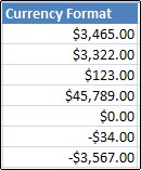
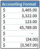
The Accounting number format in Excel is like the Currency format and can be connected to numbers wherever required. The contrast between the Accounting number format and the Currency format is that the Accounting format inserts the dollar sign. For instance, the extreme left end of the cell showcases zero as a dash. However, the format numbers are the same as the currency.

You can show a number with the default currency symbol by choosing the cell or the scope of cells. After that, click on Excel.
It has several contrasts that make it less demanding to do accounting. For example, demonstrating zero values as dashes, adjusting all the currency symbols and decimal places, and showing negative sums in enclosures.
Excel’s standard Accounting number format contains two decimal points and a thousand separators and locks the dollar sign to the extreme left half of the cell. Negative numbers are shown in enclosures.
To apply the Excel Accounting number format in a spreadsheet program, feature every cell and click “Accounting Number Format” under formatting choices.

What is the Accounting Number Format Excel?
- How to Apply Accounting Number Format in Excel?
- Shortcut Keys to Use Accounting Number Format in Excel
- Advantages of Using Accounting Number Format in Excel
- Disadvantages of Using Accounting Number Format in Excel
- Things to Remember While Using Accounting Number Format Excel
- Recommended Articles

How to Apply Accounting Number Format in Excel?

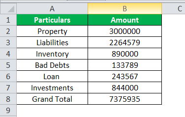
You can download this Accounting Number Format Excel Template here – Accounting Number Format Excel Template

Below are the steps for applying for the account number in Excel: –

Enter the values in Excel to use the Accounting number format.
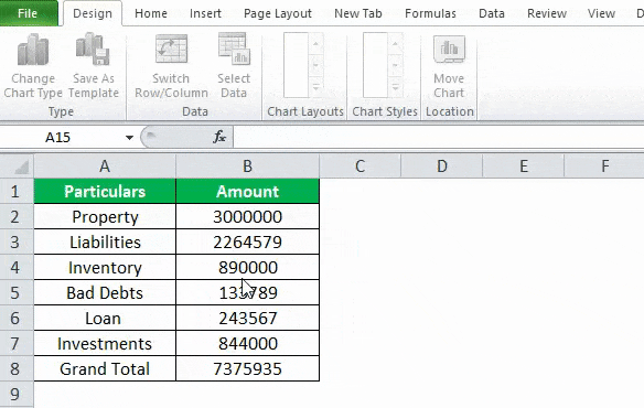
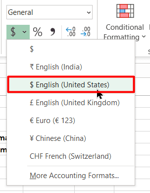
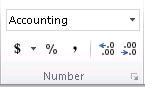
First, we can use the Accounting number format in Excel in the “Account Number Format” button on the “Home tab” of the ribbon. Select the cells, click on the “Home” tab, and select “Accounting” from the Number Format drop-down.
On clicking on “Accounting”, it may give us the accounting format value.
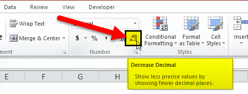
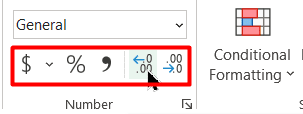
If you want to remove the decimal, click on the ‘Decrease Decimal’ option.
We can see the value without decimals by removing the decimal below.
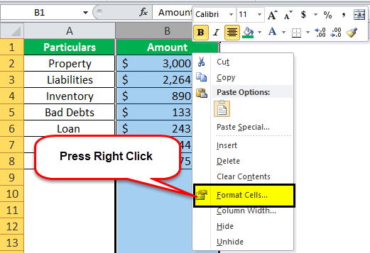
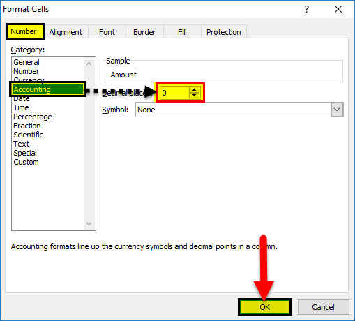
We can also remove the dollar or currency symbol from a value. To do that, press right-click and go to the “Format Cells” option in the dialog box.
Choose the “Accounting” option under the “Format Cells.” Choose the symbol. Choose “None” if the dollar sign with values is not needed. Then, click OK.
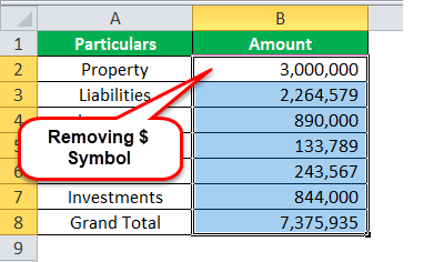
Below is the formatted data after removing symbols and decimal points.

Shortcut Keys to Use Accounting Number Format in Excel

Select the cells which need a format.
Press the Alt key that enables the commands on the ExcelVLOOKUP function, IF condition, CONCATENATE function, find MAXIMUM and MINIMUM values are the most commonly used excel commands.read more ribbon.

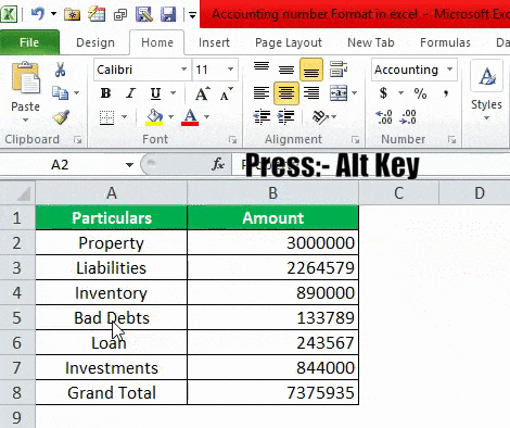
Press H to select the Home tab in the Excel ribbonThe ribbon is an element of the UI (User Interface) which is seen as a strip that consists of buttons or tabs; it is available at the top of the excel sheet. This option was first introduced in the Microsoft Excel 2007.read more enabling Excel’s Home tab.
Press 9 to decrease the decimal point in values, and press 0 to increase.
To open the format cells dialog box, press Ctrl+1.
Click ‘None’ under option format cellsFormatting cells is an important technique to master because it makes any data presentable, crisp, and in the user’s preferred format. The formatting of the cell depends upon the nature of the data present.read more to show a monetary valueMonetary value refers to the value of a product or service measured in terms of money. read more without a currency symbol.
Similar to the Currency format, the accounting group is utilized for financial qualities. In any case, this arrangement adjusts the currency symbol and decimal purposes of numbers in a section. Likewise, the accounting design shows zeros as dashes and negative numbers in brackets. Like the currency organization, we can determine the number of decimal spots needed and whether to utilize a thousand separators. We cannot change the default show of negative numbers except if we make a custom number organization.

Advantages of Using Accounting Number Format in Excel

It helps to customize it with or without the symbol.
It helps in showing the correct value with decimal points.
It is just a three-step process.
It is effortless and convenient to use.

Disadvantages of Using Accounting Number Format in Excel

This Excel function always provides the number format with a thousand separators.
It enables the default currency and decimal points while using this function.

Things to Remember While Using Accounting Number Format Excel

Instead of choosing a range of cells, likewise can be tapped on the letter over a column to select the whole column or the number next to a column to select an entire row. Again, tap the little box to one side of “A” or above “1” to choose the whole spreadsheet.
Always check to remove unnecessary symbols.
Decimal is the user’s choice to put them in values.
A custom Excel number format changes the visual representation, such as how a cell’s value is shown. The primary value put away in a cell is not changed.
A duplicate of that format is created when modifying work in Excel format. The first number format cannot be changed or erased.
Custom number formats only affect how a number is shown in the worksheet and do not affect the original value of the number.
Any cells showing in the workbook formatted with the removed custom format can be shown in the default general format in the workbook.

Transcript

In this lesson we’ll take a look at the Accounting format. Like the Currency format, the Accounting number format is designed for numbers with currency symbols. The main difference between Currency and Accounting formats is that Accounting aligns currency symbols to the left in each cell, and displays zero values with a hyphen.

Let’s take a look.

Let’s start off by copying a set of numbers in General format across our table.

Then let’s apply Accounting format to the columns C through H. The easiest way to apply Accounting is to use the Number Format menu on the ribbon.

Now let’s select cells in column D and check the options available for Accounting in the Format Cells dialog box. Like the Currency format, the Accounting format provides options for decimal places and a currency symbol, and it automatically uses a comma to separate thousandths. Unlike Currency, there are no options for negative numbers. The Accounting format places parentheses around all negative numbers by default.

Let’s set decimal places to zero. Like Number and Currency formats, we can also adjust decimal places up and down on the ribbon.

Because parentheses are automatic for negative numbers, there are no options to set in column E.

When it comes to setting the currency symbol for the Accounting format, we have some new options. There are shortcuts on the ribbon for several common currency symbols, and we can use these shortcuts for the British Pound and Euro.

Remember, using these buttons will automatically apply the Accounting number format, if it’s not already applied.

To set a currency symbol of None, or to set other currencies, use the Format Cells dialog box.

Источник

Home > Microsoft Excel > How to Apply the Accounting Number Format in Excel? (3 Best methods)

Note: This tutorial on how to apply the accounting number format in Excel is suitable for all versions of Excel including Office 365.

Excel is one of the most used spreadsheet applications cutting across industries. But it has a very special and popular status in business and accounting.

This is because it has many built-in accounting friendly features that add up to a very smooth user experience.

One such important feature is the Accounting Number Format.

Related:

How to Enable Excel Dark Mode? 3 Simple Steps

How to Add Error Bars in Excel? 7 Best Methods

How to Superscript in Excel? (9 Best Methods)

In this tutorial, I’ll show you how to use the accounting number format in the proper and easy way. I’ll cover:

What is the Accounting Number Format in Excel?
Accounting Number Format in Excel vs Currency Format
How to Apply the Accounting Number Format in Excel?
- Accounting Number Format Button
- Dropdown in the Number Group
- Accounting Format Using the Format Cells Dialogue Box
Important Note on the Accounting Number Format in Excel

You can download the practice Accounting Number Format Excel sheet here and follow along with me.

Watch this short video to learn how to apply the accounting number format in Excel

What is the Accounting Number Format in Excel?

Now, you may be wondering what is so special about this accounting number format that it demands a separate guide.

Let me explain.

Excel has built-in formatting options for various data types like numbers, texts, dates etc. For data variables dealing with money, it has the following two formatting options:

Currency Format
Accounting Number Format.

Though they may appear similar at first glance, upon closer examination, they have some important differences.

What sets the accounting number format apart is its perfect sense of alignment. That is the currency symbol and the decimal points are perfectly aligned in the whole column, making it easier to read.

Accounting Number Format in Excel vs Currency Format

Both the accounting and currency formats add a currency symbol, commas, and decimal points.

However, there are some differences that separate these two. Here is the list of differences between the currency format and the accounting number format in Excel.

Accounting Number Format Excel vs Currency Format

The currency format displays negative values as it is, whereas the accounting format displays them inside brackets. This is in accordance with the international accounting standard.

The currency format displays zero values as it is, whereas the accounting format replaces them with a ‘-’ as per the International Accounting Standards (IAS).

The currency symbol appears right next to the number in the currency format. Whereas, it appears at the extreme left end in the accounting number format.

The decimal points and comma separators are perfectly aligned in the accounting number format. That is not the case with the currency format.

Also Read:

How to Use the Excel Fill Handle Easily? (Top 3 Uses with Examples)

How to Shade Every Other Row in Excel? (5 Best Methods)

VLOOKUP for Dummies (or newbies)

How to Apply the Accounting Number Format in Excel?

There are three ways to apply the accounting format in Excel:

Accounting Number Format Button
Dropdown in the Number Group
Format cells dialogue box.

Now, let us see each of these methods one by one.

How to Apply the Accounting Number Format in Excel using the Accounting Number Format Button?

Using the accounting number format button is the easiest and most straightforward method to apply the accounting number format in Excel. Here’s how to do it:

Step 1 – Select the Range of Cells

Select the cells you want to format. You can select more than one range and even the entire sheet.

Step 2 – Use the Accounting Number Format Button

Locate and click on the Accounting Number Format button in the Number group under the Home tab. This will apply your regional currency to the format. The keyboard shortcut is Alt+H+AN.

Step 3 – Set the Accounting Currency

If you need some other currency to be applied, click on the dropdown button next to the Accounting Number Format button and click on the suitable currency.

Step 4 – Increase or Decrease the Decimals

Now, increase or decrease the decimal values as per your requirements. Please note that you cannot change the appearance of the comma separators. Keyboard shortcuts are Alt+H+0 or Alt+H+9 to increase or decrease the decimal values respectively.

Dropdown in the Number Group

Another way to access the accounting format option is to use the dropdown menu in the number group.

Select the cells you want to format.

Locate and click on the Dropdown menu button in the Number group under the Home tab.

Now, select Accounting from the list of formats appearing in the Dropdown menu. This will apply your regional currency to the format. The keyboard shortcut is Alt+H+N+A, followed by an Enter.

Accounting Number Format in Excel using the Dropdown menu

If you want to change the currency, click on the dropdown button next to the Accounting Number Format button and click on the suitable currency. g

Now, increase or decrease the decimal values as per your requirements. Please note that you cannot change the appearance of the comma separators.

Accounting Format Using the Format Cells Dialogue Box

The format cells dialogue box is another effective way to apply the accounting format in Excel.

To do this, just follow these steps:

Select the cells you want to format.

Right-click on the selection and click on the Format cells options in the right-click menu. Alternatively, you can use the keyboard shortcut Ctrl+1.

Select Format Cells from the right-click context menu

In the Format Cells dialogue box, select the Number tab.

Select ‘Accounting’ under ‘Category’.

Choose currency symbol and number of decimal places in the Format Cells dialogue box

Choose your currency symbol and the number of decimal places and click OK.

Important Note on the Accounting Number Format in Excel

The accounting format is applicable only to numerical values.
Applying the accounting format to a blank cell will convert any future values of the cell to the accounting format.
The accounting format has no effect on the original cell values. It simply changes the appearance of the values.

Suggested Reads:

How to Group Worksheets in Excel? (In 3 Simple Steps)

Easily Make a Bullet Chart in Excel—2 Examples

Closing Thoughts

That’s all folks. These are the different methods to apply the accounting number format in Excel. If you have any questions regarding this or any other Excel feature, please let us know in the comments. We are always happy to help.

If you need more high-quality Excel guides, please check out our free Excel resources centre.

Ready to dive deep into Excel? Simon Sez IT has been teaching Excel for over ten years. For a low, monthly fee you can get access to 100+ IT training courses. Click here for advanced Excel courses with in-depth training modules.

Simon Calder

Chris “Simon” Calder was working as a Project Manager in IT for one of Los Angeles’ most prestigious cultural institutions, LACMA.He taught himself to use Microsoft Project from a giant textbook and hated every moment of it. Online learning was in its infancy then, but he spotted an opportunity and made an online MS Project course — the rest, as they say, is history!

Источник

Содержание

Format numbers as currency
In this article
Format numbers as currency
Remove currency formatting
What’s the difference between the Currency and Accounting formats?
Create a workbook template with specific currency formatting settings
Save the workbook as a template
Create a workbook based on the template
Top Excel Templates for Accounting
Accounting Journal Template
Accounts Payable Template
Accounts Receivable Template
Bill To Invoice Template
Bill of Lading Template
Billing Statement Template
Cash Flow Statement Template
Cash Flow Forecast Template
Expense Report Template
Income Statement Template
Payment Schedule Template
Simple Balance Sheet Template
Travel Itinerary Template
Save Hours of Manual Work with Smartsheet

Format numbers as currency

If you want to display numbers as monetary values, you must format those numbers as currency. To do this, you apply either the Currency or Accounting number format to the cells that you want to format. The number formatting options are available on the Home tab, in the Number group.

Format numbers as currency

You can display a number with the default currency symbol by selecting the cell or range of cells, and then clicking Accounting Number Format in the Number group on the Home tab. (If you want to apply the Currency format instead, select the cells, and press Ctrl+Shift+$.)

If you want more control over either format, or you want to change other aspects of formatting for your selection, you can follow these steps.

Select the cells you want to format

On the Home tab, click the Dialog Box Launcher next to Number.

Tip: You can also press Ctrl+1 to open the Format Cells dialog box.

In the Format Cells dialog box, in the Category list, click Currency or Accounting.

In the Symbol box, click the currency symbol that you want.

Note: If you want to display a monetary value without a currency symbol, you can click None.

In the Decimal places box, enter the number of decimal places that you want for the number. For example, to display $138,691 instead of $138,690.63 in the cell, enter 0 in the Decimal places box.

As you make changes, watch the number in the Sample box. It shows you how changing the decimal places will affect the display of a number.

In the Negative numbers box, select the display style you want to use for negative numbers. If you don’t want the existing options for displaying negative numbers, you can create your own number format. For more information about creating custom formats, see Create or delete a custom number format.

Note: The Negative numbers box is not available for the Accounting number format. That’s because it is standard accounting practice to show negative numbers in parentheses.

To close the Format Cells dialog box, click OK.

If Excel displays ##### in a cell after you apply currency formatting to your data, the cell probably isn’t wide enough to display the data. To expand the column width, double-click the right boundary of the column that contains the cells with the ##### error. This automatically resizes the column to fit the number. You can also drag the right boundary until the columns are the size that you want.

Remove currency formatting

If you want to remove the currency formatting, you can follow these steps to reset the number format.

Select the cells that have currency formatting.

On the Home tab, in the Number group, click General.

Cells that are formatted with the General format do not have a specific number format.

What’s the difference between the Currency and Accounting formats?

Both the Currency and Accounting formats are used to display monetary values. The difference between the two formats is explained in the following table.

When you apply the Currency format to a number, the currency symbol appears right next to the first digit in the cell. You can specify the number of decimal places that you want to use, whether you want to use a thousands separator, and how you want to display negative numbers.

Tip: To quickly apply the Currency format, select the cell or range of cells that you want to format, and then press Ctrl+Shift+$.

Like the Currency format, the Accounting format is used for monetary values. But, this format aligns the currency symbols and decimal points of numbers in a column. In addition, the Accounting format displays zeros as dashes and negative numbers in parentheses. Like the Currency format, you can specify how many decimal places you want and whether to use a thousands separator. You can’t change the default display of negative numbers unless you create a custom number format.

Tip: To quickly apply the Accounting format, select the cell or range of cells that you want to format. On the Home tab, in the Number group, click Accounting Number Format . If you want to show a currency symbol other than the default, click the arrow next to the Accounting Number Format button and then select another currency symbol.

Create a workbook template with specific currency formatting settings

If you often use currency formatting in your workbooks, you can save time by creating a workbook that includes specific currency formatting settings, and then saving that workbook as a template. You can then use this template to create other workbooks.

Create a workbook.

Select the worksheet or worksheets for which you want to change the default number formatting.

How to select worksheets

Click the sheet tab.

If you don’t see the tab that you want, click the tab scrolling buttons to display the tab, and then click the tab.

Two or more adjacent sheets

Click the tab for the first sheet. Then hold down Shift while you click the tab for the last sheet that you want to select.

Two or more nonadjacent sheets

Click the tab for the first sheet. Then hold down Ctrl while you click the tabs of the other sheets that you want to select.

All sheets in a workbook

Right-click a sheet tab, and then click Select All Sheets on the shortcut menu.

Tip When multiple worksheets are selected, [Group] appears in the title bar at the top of the worksheet. To cancel a selection of multiple worksheets in a workbook, click any unselected worksheet. If no unselected sheet is visible, right-click the tab of a selected sheet, and then click Ungroup Sheets.

Select the specific cells or columns you want to format, and then apply currency formatting to them.

Make any other customizations that you like to the workbook, and then do the following to save it as a template:

Save the workbook as a template

If you’re saving a workbook to a template for the first time, start by setting the default personal templates location :

Click File, and then click Options.

Click Save, and then under Save workbooks, enter the path to the personal templates location in the Default personal templates location box.

This path is typically: C:UsersPublic DocumentsMy Templates.

Once this option is set, all custom templates you save to the My Templates folder automatically appear under Personal on the New page ( File > New).

Click File, and then click Export.

Under Export, click Change File Type.

In the Workbook File Types box, double-click Template.

In the File name box, type the name you want to use for the template.

Click Save, and then close the template.

Create a workbook based on the template

Click File, and then click New.

Double-click the template you just created.

Excel creates a new workbook that is based on your template.

Источник

Top Excel Templates for Accounting

December 29, 2015

In this article, you’ll find the most comprehensive list of free, downloadable accounting templates for a variety of use cases.

Accounting Journal Template

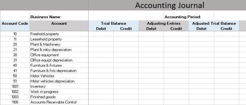
An accounting journal is an accounting worksheet that allows you to track each of the steps of the accounting process, side by side. This accounting journal template includes each step with sections for their debits and credits, and pre-built formulas to calculate the total balances for each column.

We’ve also included links to similar accounting templates in Smartsheet, a spreadsheet-inspired work management tool that makes accounting processes even easier and more collaborative than Excel.

Accounts Payable Template

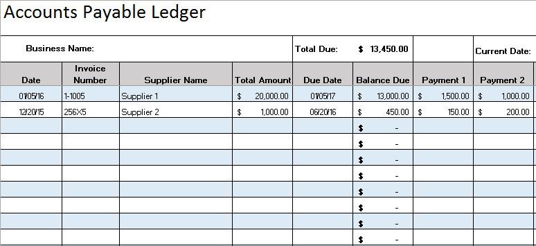
When making large purchases for items like inventory, supplies, or equipment it may be necessary to do so on credit, which could result in multiple monthly payments made to different vendors or suppliers, due on different dates. Using this accounts payable template will help to keep track of what you owe to each party, and will provide a quick look at the total outstanding balances and due dates.

Accounts Receivable Template

Every company should have a process in place to manage the outstanding balances owed to them. Using this accounts receivable template will help streamline the process by providing a place for you to track the amounts due to your company and help prioritize collection efforts.

Bill To Invoice Template

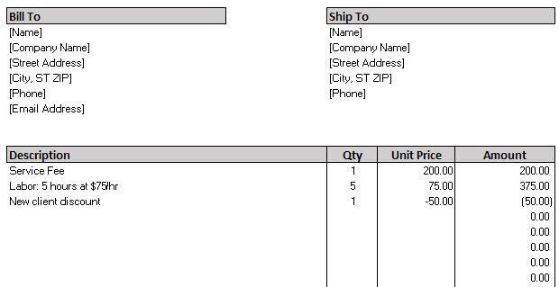
For any company providing goods or services, using an invoice that looks professional and can be customized to fit your needs, is important. This simple bill template will help you get started quickly. Add your company details and payee information, provide an itemized list of the description, quantity, and price of each item you are charging for, and include directions on how your customer may remit payment.

Bill of Lading Template

A bill of lading is a document detailing how goods are being shipped from a seller to a recipient. It includes details about the items being shipped, the quantity of items included in the shipment, and the destination address. Use a bill of lading template to ensure you complete this document for each shipping transaction. This template includes a signature section that should be signed by you, then the shipping company, and finally the recipient, so that if the shipment is lost, the signature detail will help identify at what point it was lost and who was liable.

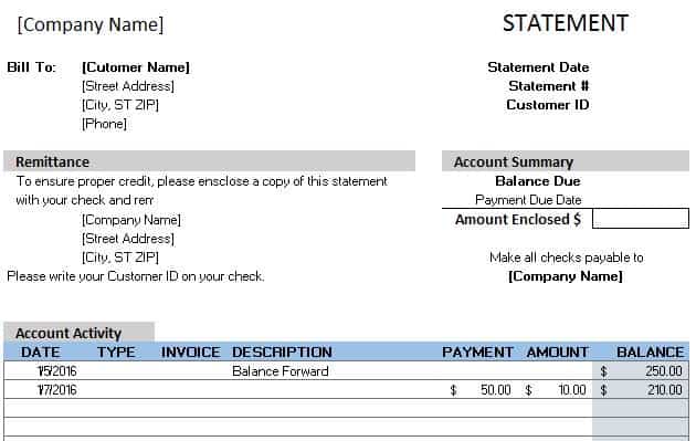
Billing Statement Template

A billing statement is helpful if you receive regular bi-monthly or monthly payments from your customers. Use this billing statement template to track customer invoices, account details, and billing status, all in one location. Additionally, this template looks professional and is customizable to match your needs.

Cash Flow Statement Template

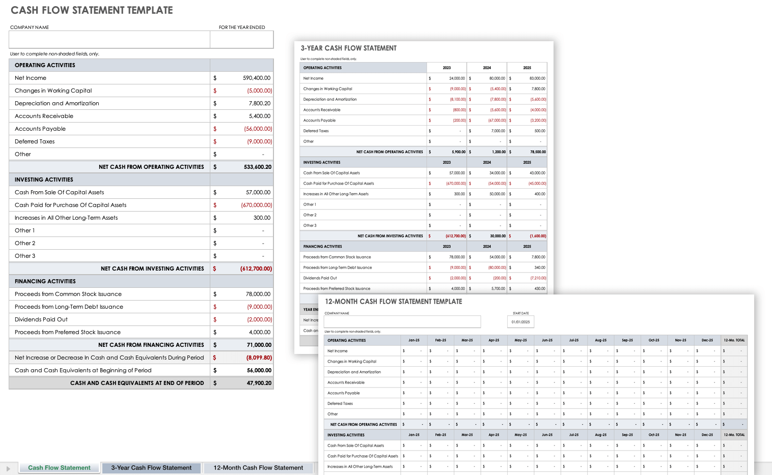
A cash flow statement is important to provide a good picture of the inflow and outflow of cash within your company. It shows where the money came from (cash receipts) and where the money went to (cash paid). Use a cash flow statement template, in conjunction with your balance sheet and income statement, to provide a comprehensive look into the financial status of your company. This cash flow template includes two additional worksheets to track month-to-month and year-to-year cash flow.

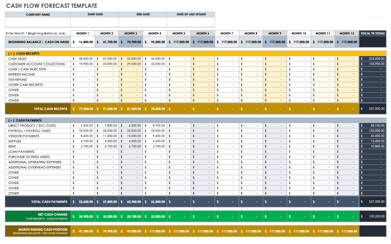
Cash Flow Forecast Template

Creating a cash flow forecast can be helpful for managing your business’ finances. It enables you to estimate how much money your business will make and spend at any given point, and will allow you to take the appropriate steps to ensure that your cash outflow is not more than your inflow. Use a simple cash flow forecast template to get started quickly. Be sure you include all income including revenue and investments, and account for all expenses including fixed costs.

Expense Report Template

A simple expense report is helpful to keep track of business expenses for an individual, department, project, or company, and provides a quick way to document and track expense details. You can require that your team submit monthly expense reports or as the expenses are accrued. Use this expense report template to quickly input specific expense details and obtain approvals as needed.

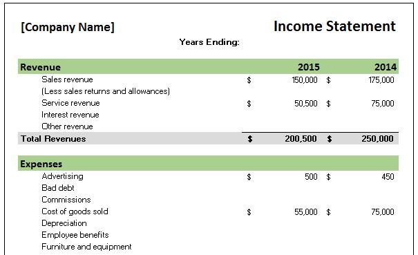
Income Statement Template

An income statement, or profit and loss statement, provides a look into the financial performance of a company over a period of time. The statement provides a summary of the company’s revenue and expenses, along with the net income. Use this income statement template to create a single-step statement that groups all revenue and expenses, and is helpful for businesses of all sizes.

Payment Schedule Template

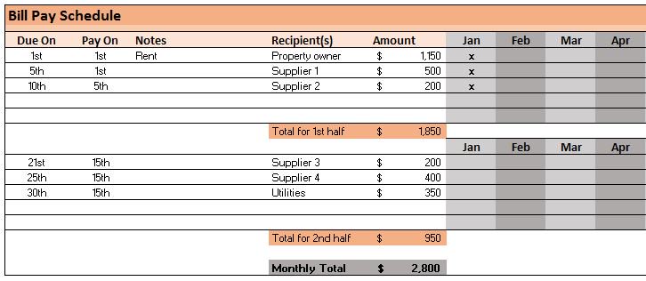
You will likely have multiple bills to pay in a month, to different companies and on different dates. It is important to have a way to track when specific bills are due, the amount that is due, and to whom. Use a simple payment schedule template to track these details. This payment schedule template will help you remember when each bill is due and be able to budget accordingly.

Simple Balance Sheet Template

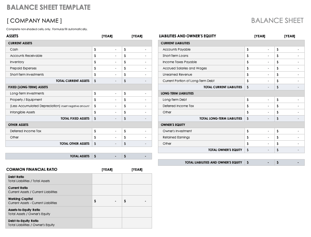
A simple balance sheet template provides a quick snapshot of a company’s financial position, at a given moment. Use this balance sheet template to summarize the company’s assets, liabilities, and equity, and give investors an idea of the health of the company.

Travel Itinerary Template

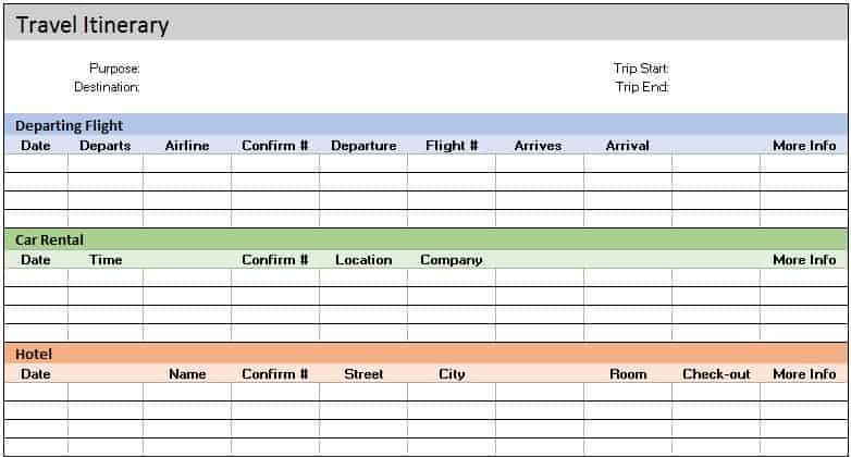
Whenever you or your team are scheduled for business trips, it’s helpful to have a travel itinerary that lists the details for transportation, lodging, car rentals, meetings and more. Use a simple business travel itinerary template to keep all of these details in one location, and be able to share the details with important stakeholders.

Save Hours of Manual Work with Smartsheet

Empower your people to go above and beyond with a flexible platform designed to match the needs of your team — and adapt as those needs change.

The Smartsheet platform makes it easy to plan, capture, manage, and report on work from anywhere, helping your team be more effective and get more done. Report on key metrics and get real-time visibility into work as it happens with roll-up reports, dashboards, and automated workflows built to keep your team connected and informed.

When teams have clarity into the work getting done, there’s no telling how much more they can accomplish in the same amount of time. Try Smartsheet for free, today.

Источник

Do you work in finance and need to apply the accounting number format to your data?

This post is going to show you how to add the accounting format to your numbers in Excel!

Excel offers users a variety of number formatting options. This is because there are many types of numbers such as dates, percentages, or currencies. Different number formatting allows you to present the data appropriately.

The accounting format is appropriate to use with currency values and has several great features that make comparing numbers super easy.

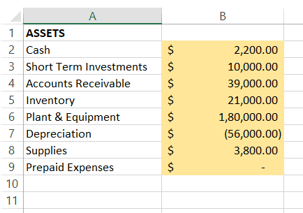
Zeros are shown as a dash. This makes 0 value very easy to spot.
A currency symbol such as $ is added.
The currency symbol is aligned to the left of the cell.
The numbers are aligned to the right of the cell.
The currency symbol and decimal are aligned across a column.

Get your copy of the example workbook used in this post to follow along.

Add Accounting Format from the Home Tab

The accounting number format is a very commonly used format. Because of this, it is made easily accessible from the ribbon commands. You can find this in the Home tab.

You can follow these steps to apply the accounting number format from the Home tab.

Select the range of values to which you want to apply the accounting format.

Go to the Home tab.
Click on the format dropdown menu found in the Number section of the ribbon.

Choose the Accounting option.

Your selected numbers will now appear in the accounting format!

Add Accounting Format from Format Cells Menu

If you are applying any sort of format in Excel, you should familiarize yourself with the Format Cell menu.

This is where you will be able to access any type of cell format such as borders, fill color, font color, etc. You will also find all the available number formatting options here.

Follow these steps to apply the accounting format with the Format Cells menu.

Select the range of numbers in your sheet.
Open the Format Cells menu. There are a couple of ways to do this.
- Right-click and choose Formal Cells.
- Press the Ctrl + 1 keyboard shortcut.
- Go to the Home tab and click on the Launch icon in the lower right corner of the Numbers section.
Go to the Numbers tab in the Format Cells menu.
Select the Accounting option in the Category list.
Choose the number of Decimal places to include and the currency Symbol to display.
Press the OK button.

Your numbers are now formatted with the accounting format!

📝 Note: Using the Format Cells menu gives you the option to select other currency symbols that aren’t available in the Home tab.

Add Accounting Format from the Quick Access Toolbar

If you work in the accounting or financial industry, then you might be using the accounting format constantly.

Having this easily accessible will save you some significant time!

You can add the format drop-down selector to the Quick Access Toolbar, and this way it will be available wherever you are in the ribbon.

Right-click on the dropdown button and select Add to Quick Access Toolbar from the options.

This will add a small dropdown list into the Quick Access Toolbar area and you will be able to use this anytime!

Add Accounting Format with a Keyboard Shortcut

There is no dedicated keyboard shortcut for applying the accounting format in Excel.

But you can use the Alt hotkeys to access the format from the Home tab ribbon.

Press the sequence Alt, H, N, A. This will select the Accounting format from the dropdown in the Home tab. Then you will need to press the Enter key to accept the selection.

Add Accounting Format with a Custom Format

Another option you can use is a Custom Format to create your own accounting format.

Why create a custom format when there is already an accounting format?

The accounting format doesn’t allow you to show negative numbers with a red font or inside parentheses. Since there is only a small dash character before the currency symbol, negative numbers can be easy to miss.

Follow these steps to create a custom accounting format with red negative numbers inside parentheses.

Select the numbers to format.
Press the Ctrl + 1 keyboard shortcut to open the Format Cells menu.
Go to the Numbers tab.
Select the Custom option in the Category list.

_ $* #,##0.00 _ ;[Red] $* (#,##0.00)_ ;_ $* "-"?? _ ;_ @_

Paste the above format string into the Type input.
Press the OK button.

⚠️ Warning: The custom format string has a space character at the end and this needs to be included!

positive;negative;zero;text

The format syntax consists of 4 parts separated by a ; character. They determine what the positive, negative, zero, and any text values will look like.

Each part contains an asterisks character followed by a space $* . The asterisk is a repeater character and it means the space after it will be repeated to fill the cell.

You’ll also notice the [red] prefix has been added to the negative section. This will result in any negative values displaying in red font.

The ?? in the zero section ensures the dash character - will line up with any decimals in other cells.

This results in a custom accounting format where the negative numbers are immediately obvious!

If you look very closely at the results, you will see the decimal points don’t line up exactly across the column though.

This is because the positive part of the format string uses a space as a placeholder while the negative part uses a closing parentheses ). These characters are slightly different sizes and result in misalignment!

This can be fixed by using a monospaced font such as Courier New. This ensures each character is the same width and everything will line up nicely across the column.

Select the numbers and go to the Home tab and select Courier New from the dropdown in the Font section.

Add Accounting Format with the TEXT Function

Suppose you want to cast your numbers to text values and include the accounting format. This is possible using the TEXT function.

The TEXT function uses the same format string syntax to convert a number to a formatted text value.

The process will be more complicated than the custom format though as the TEXT function doesn’t allow the use of the asterisks * to repeat characters. This means you will have to calculate how many spaces to insert for each number to format!

=LET(
    maxlength, 15,
    text, TEXT(D3," $ #,##0.00__ ; $ (#,##0.00)_ ; $ ""-    """),
    length, LEN(text),
    diff, MAX(0,maxlength-length),
    newtext, SUBSTITUTE(text,"$ ","$"&REPT(" ",diff)),
    newtext
)

The above formula will convert the number in cell D3 to a text value in accounting format where the negative numbers are in parentheses.

This will also require that you change to a monospaced font such as Courier New to get the decimal points to line up across the column.

This formula will calculate the length of the formatted number with a single space and then determine how many extra spaces to insert to make sure there are a total of 15 characters.

You will need to update the maxlength, 15, section of the formula to accommodate formatting larger numbers.

📝 Note: Using the [red] prefix in the format syntax is not possible in the TEXT function. But you could use conditional formatting to achieve this same effect.

Conclusions

Account format is a common number format used across the financial industry to help make the numbers easier to read.

There are several ways to add the accounting format to your selected numbers. The Home tab or Format Cells menu will be the most straightforward way.

But if you need to use the accounting format with negative values in parentheses, then you will need to create a Custom Fformat or use the TEXT function.

Do you use the accounting format for your numbers? Do you know any other ways to apply this format? Let me know in the comments below!

About the Author

John MacDougall

John is a Microsoft MVP and qualified actuary with over 15 years of experience. He has worked in a variety of industries, including insurance, ad tech, and most recently Power Platform consulting. He is a keen problem solver and has a passion for using technology to make businesses more efficient.

Источник

What is the Accounting Number Format Excel?

Table of contents

How to Apply Accounting Number Format in Excel?

Shortcut Keys to Use Accounting Number Format in Excel

Advantages of Using Accounting Number Format in Excel

Disadvantages of Using Accounting Number Format in Excel

Things to Remember While Using Accounting Number Format Excel

Recommended Articles

Transcript

What is the Accounting Number Format in Excel?

Accounting Number Format in Excel vs Currency Format

How to Apply the Accounting Number Format in Excel?

How to Apply the Accounting Number Format in Excel using the Accounting Number Format Button?

Step 1 – Select the Range of Cells

Step 2 – Use the Accounting Number Format Button

Step 3 – Set the Accounting Currency

Step 4 – Increase or Decrease the Decimals

Dropdown in the Number Group

Accounting Format Using the Format Cells Dialogue Box

Important Note on the Accounting Number Format in Excel

Closing Thoughts

Simon Calder

Format numbers as currency

In this article

Format numbers as currency

Remove currency formatting

What’s the difference between the Currency and Accounting formats?

Create a workbook template with specific currency formatting settings

Save the workbook as a template

Create a workbook based on the template

Top Excel Templates for Accounting

Accounting Journal Template

Accounts Payable Template

Accounts Receivable Template

Bill To Invoice Template

Bill of Lading Template

Billing Statement Template

Cash Flow Statement Template

Cash Flow Forecast Template

Expense Report Template

Income Statement Template

Payment Schedule Template

Simple Balance Sheet Template

Travel Itinerary Template

Save Hours of Manual Work with Smartsheet

Add Accounting Format from the Home Tab

Add Accounting Format from Format Cells Menu

Add Accounting Format from the Quick Access Toolbar

Add Accounting Format with a Keyboard Shortcut

Add Accounting Format with a Custom Format

Add Accounting Format with the TEXT Function

Conclusions

About the Author