
In this article we will learn how to format the cells which is containing the formulas in Microsoft Excel.
To format the cells which contain formulas, we use the Conditional Formatting feature along with the ISFORMULA function in Microsoft Excel.
Conditional Formatting: —Conditional Formatting is used to highlight the important points with color in a report based on certain conditions.
ISFORMULA-This function is used to check whether a cell reference contains a formula and it returns a True or False.
For Example — We have this Excel data as shown below —
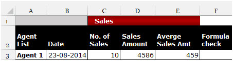
We need to check whether cell E3 containsa formula or not.
To check, follow the below given steps:-
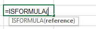
- Select the cell F3 and write the formula.
- =ISFORMULA(E3), press Enter on the keyboard.
- The function will return true.
- It means cell E3 contains a formula.
Let’s take an example to understand how we can highlight the cells which contain formulas.
We have data in range C2:G7, in which column C contains Agents name, column D contains No. of sales, column E contains sales amount and column F contains Average sales amount. We need to highlight the cells which contain the formula.
Follow the below given steps:-
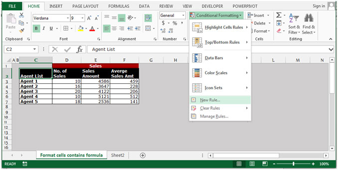
- Select the data range C3:F7.
- Go to the Home Tab.
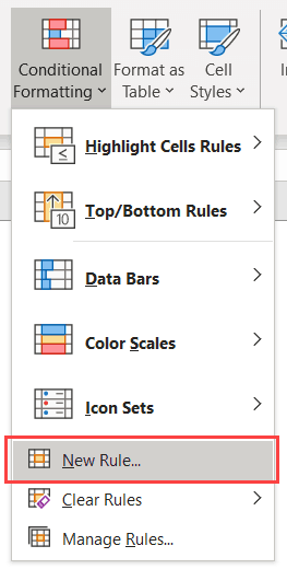
- Select Conditional Formatting from the Styles group.
- From the Conditional formatting drop down menu, select New Rule.
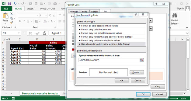
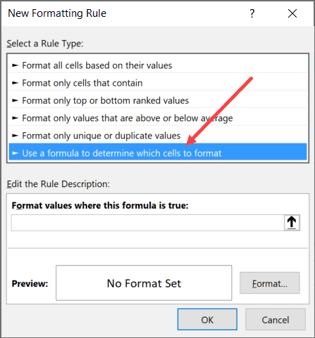
- The New Formatting Rule dialog box will appear.
- Click on “Use a formula to determine which cells to format” from Select a Rule type.
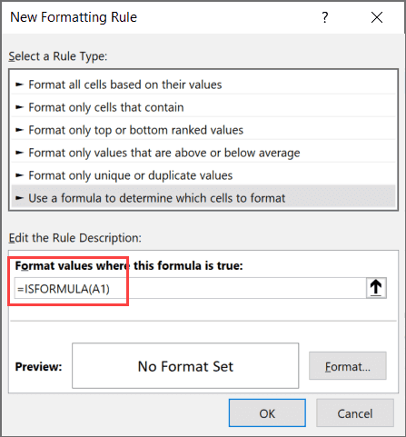
- Write the formula in Formula tab.
- =ISFORMULA(C3:F7)
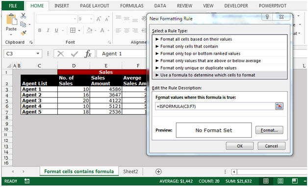
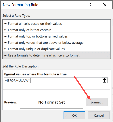
- Click on Format button.
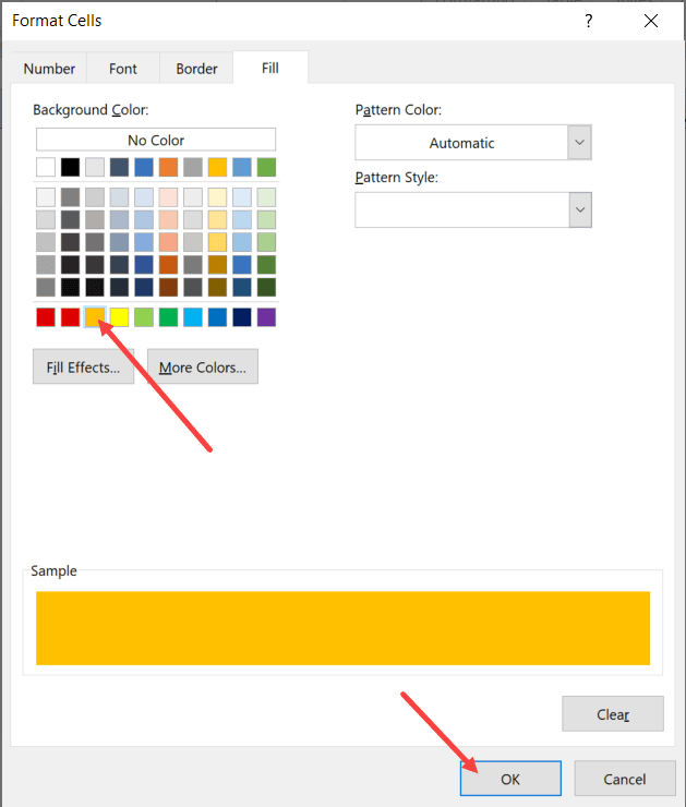
- The Format Cells dialog box will appear.
- In the Fill tab, choose the color as per the requirement.
- Click on OK on the New Formatting Rule dialog box.
- Click on OK on the Format Cells dialog box.
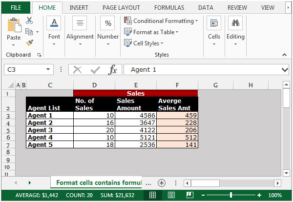
All cells which contain formulas will get highlighted with the chosen color. This is the way we can highlight the cells containing formulas in an Excel sheet by using the Conditional Formatting option along with the ISFORMULA function.
![]()
If you liked our blogs, share it with your friends on Facebook. And also you can follow us on Twitter and Facebook.
We would love to hear from you, do let us know how we can improve, complement or innovate our work and make it better for you. Write us at info@exceltip.com
To control more precisely what cells will be formatted, you can use formulas to apply conditional formatting.
Want more?
Use conditional formatting
Manage conditional formatting rule precedence
To control more precisely what cells will be formatted, you can use formulas to apply conditional formatting.
In this example, I am going to format the cells in the Product column if the corresponding cell in the In stock column is greater than 300.
I select the cells I want to conditionally format.
When you select a range of cells, the first cell you select is the active cell.
In this example, I selected from B2 through B10, so B2 is the active cell. We’ll need to know that shortly.
Create a new rule, select Use a formula to determine which cells to format. Since B2 is the active cell, I type =E2>300.
Note that in the formula, I used the relative cell reference E2 to make sure the formula adjusts to correctly format the other cells in column B.
I click the Format button and choose how I want to format the cells. I am going to use a blue fill.
Click OK to accept the color; click OK again to apply the format.
And the cells in the Product column, where the corresponding cell in column E is greater than 300, are conditionally formatted.
When I change a value in column E to greater than 300, the conditional formatting in the Product column automatically applies.
You can create multiple rules that apply to the same cells.
In this example, I want different fill colors for different ranges of scores.
I select the cells I want to apply a rule to, create a new rule that uses the rule type Use a formula to determine which cells to format.
I want to format a cell if its value is greater than or equal to 90.
The active cell is B2, so I enter the formula =B2>=90.
And configure the rule to apply a green fill when the formula is true for a cell. The cell that has a value greater than or equal to 90 is filled with green.
I create another rule for the same cells, but this time, I want to format a cell if its value is greater than or equal to 80 and less than 90.
The formula is =AND(B2>=80,B2<90).
And I choose a different fill color.
I create similar rules for 70 and 60. The last rule is for values less than 60.
The cells are now a rainbow of colors, and these are the rules we just created to enable this.
Up next, Manage conditional formatting.
When working with formulas, there is always a possibility that someone (or even you) may delete a cell (or clear the contents of a cell/range) that has formulas in it.
Wouldn’t it be better if these cells with formulas are highlighted or formatted in a way that makes these stand out? This would help ensure you don’t end up deleting these cells by mistake.
In this tutorial, I will show you how to auto-format formulas in Excel (i.e., highlight the cells with formulas).
So let’s get started!
Autoformat Formulas using Conditional Formatting
The easiest way to autoformat cells with formulas is to use conditional formatting.
If you can somehow identify cells that have formulas, you can easily format these differently using conditional formatting.
And this is where you can use the ISFORMULA function, a function that was introduced in Excel 2013.
The ISFORMULA function checks whether a cell has a formula in it or not, and if it has a formula, then it returns TRUE (else FALSE).
Below are the steps to use this function in Conditional Formatting to autoformat formulas in Excel:
- Select the dataset in which you want to format the cells with formulas
- Click the Home tab

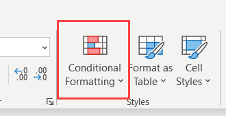
- In the Styles group, click on Conditional Formatting

- Click on New Rule

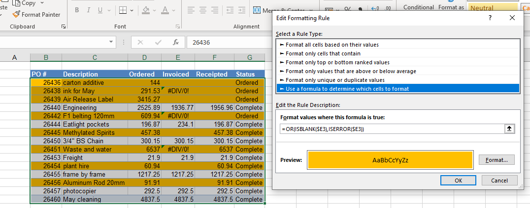
- In the New Formatting Rule dialog box that opens, select ‘Use a formula to determine which cells to format’

- In the formula field, enter the formula =ISFORMULA(A1)
- Click on the Format button
- In the Format Cells dialog box that opens, specify the formatting that you want to apply to the cells with formulas. In my case, I am using the orange cell fill color

- Click OK
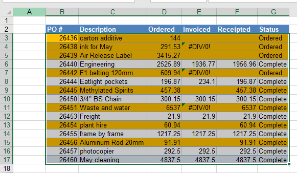
The above steps would instantly autoformat all the cells that have a formula in it.
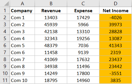
Not only this, in case you change any of the cells and add a formula to it, the color would automatically change. Since conditional formatting is dynamic and checks for each cell every time there is a change in the worksheet, the above steps make sure cells are automatically highlighted.
While this is my preferred method to autoformat formulas in Excel, there is another way as well.
Also read: How to Strikethrough in Excel (5 Ways + Shortcuts)
Autoformat Formulas using Go To Special
Unlike the Conditional formatting method, this one is not dynamic.
So when you do this once, it will select all the cells with formulas and you can format them at one go. But if now you change any cell and add a formula, that cell will not get highlighted.
Below are the steps to use Go To Special to select all cells with Formulas and then format these:
- Select the dataset in which you want to format the cells with formulas
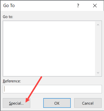
- Hit the F5 key – this will open the Go To dialog box
- Click on the Special button

- In the Go To Special dialog box, Click on Formulas

- Click OK
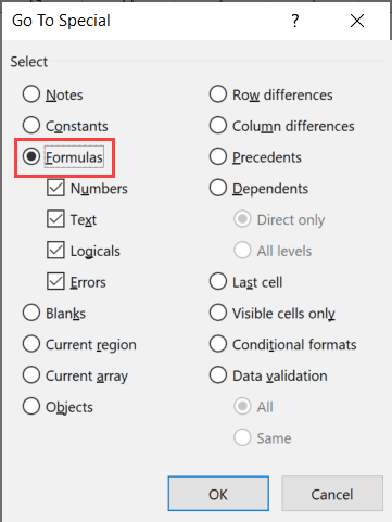
The above steps would select all the cells that have formulas in it. Once these cells are selected, you can apply whatever formatting you want. For example, you can apply a cell color or can change the font to bold.
As I mentioned, now if you add a new formula to the range, it will not get autoformatted. You will have to repeat the same process again.
Format Formulas using VBA
Another quick method to quickly format cells with formulas is by using VBA.
This method does exactly the same thing as the one the previous one (using Go To Special), but with a single line of code.
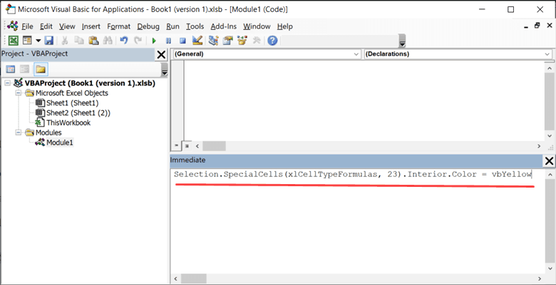
Below is the VBA code that will instantly highlight all the cells that have formulas in it in yellow color:
Selection.SpecialCells(xlCellTypeFormulas, 23).Interior.Color = vbYellow
This code first selects all the cells that have formulas and then applies the yellow color (specified by vbYellow).
Here are the steps to use this VBA macro code:
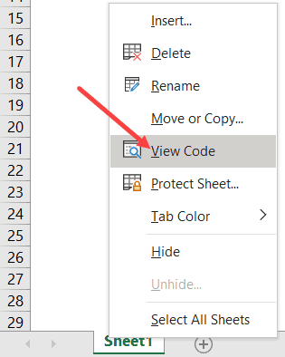
- Right-click on the active sheet tab name (the one where you have the data with formulas that you want to format).
- Click on View Code

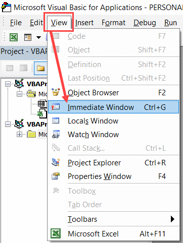
- If you don’t see the ‘Immediate window’ in the VB Editor already, click on the ‘View’ option in the menu and then click on ‘Immediate Window’

- Copy and paste the above VBA code in the ‘Immediate Window’

- Place the cursor at the end of the line
- Hit the Enter key
The above code first identifies all the cells with formulas and then applies the yellow color. You can modify the code in case you want to apply some other type of formatting.
So these are two simple ways to quickly autoformat formulas in Excel.
Hope you found this tutorial useful!
You may also like the following Excel tutorials:
- How to Format Phone Numbers in Excel
- How to Clear Contents in Excel without Deleting Formulas
- How to Delete a Comment in Excel (or Delete ALL Comments)
- Excel Showing Formula Instead of Result
- SUMPRODUCT vs SUMIFS Function in Excel
- How to Convert Decimal to Fraction in Excel
- How to Shade Every Other Row in Excel
- How to Autofill Dates in Excel (Autofill Months/Years)
- How to Apply Comma Style in Excel
- How to Increase/Decrease Indent in Excel? (Easy Shortcut)
This tutorial about cell format types in Excel is an essential part of your learning of Excel and will definitely do a lot of good to you in your future use of this software, as a lot of tasks in Excel sheets are based on cells format, as well as several errors are due to a bad implementation of it.
A good comprehension of the cell format types will build your knowledge on a solid basis to master Excel basics and will considerably save you time and effort when any related issue occurs.
A- Introduction
Excel software formats the cells depending on what type of information they contain.
To update the format of the highlighted cell, go to the “Home” tab of the ribbon and click, in the “Number” group of commands on the “Number Format” drop-down list.
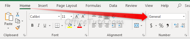
The drop-down list allows the selection to be changed.
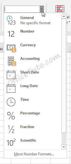
Cell formatting options in the “Number Format” drop-down list are:
- General
- Number
- Currency
- Accounting
- Short Date
- Long Date
- Time
- Percentage
- Fraction
- Scientific
- Text
- And the “More Number Formats” option.
Clicking the “More Number Formats” option brings up additional options for formatting cells, including the ability to do special and custom formatting options.
These options are discussed in detail in the below sections.
Cell format types in Excel are: General, Number, Currency, Accounting, Date, Time, Percentage, Fraction, Scientific, Text, Special (Zip Code, Zip Code + 4, Phone Number, Social Security Number), and Custom. You can get them from the “Number Format” drop-down list in the “Home” tab, or from the launcher arrow below it.
I will detail each one of them in the following sections:
1- General format
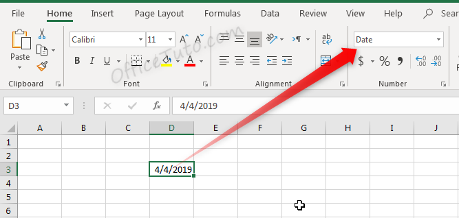
By default, cells are formatted as “General”, which could store any type of information. The General format means that no specific format is applied to the selected cell.
When information is typed into a cell, the cell format may change automatically. For example, if I enter “4/4/19” into a cell and press enter, then highlight the cell to view details about it, the cell format will be listed as “Date” instead of “General”.
Similarly, we can update a cell’s format before or after entering data to adjust the way the data appears. Changing the format of a cell to “Currency” will make it so information entered is displayed as a dollar amount.
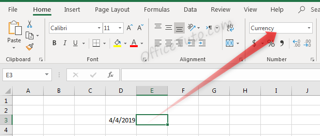
Typing a number into this cell and pressing enter will not just show that number, but will instead format it accordingly.
Before pressing enter, Excel shows the value which was typed: “4”.
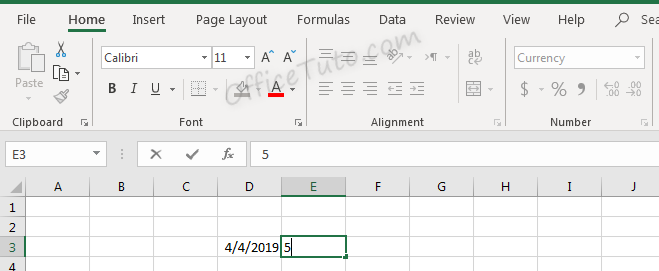
After pressing enter, the value is updated based on the formatting type selected.
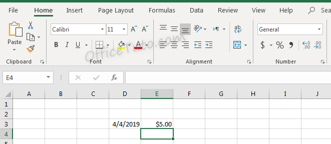
Don’t let the format type showed in the illustration at the drop-down list confusing you; it is reflecting the cell below (i.e. E4), since we validated by an Enter.
2- Number format
Cells formatted as numbers behave differently than general formatted cells. By default, when a number is entered, or when a cell is formatted as a number already, the alignment of the information within the cell will be on the right instead of on the left. This makes it easier to read a list of numbers such as the below.
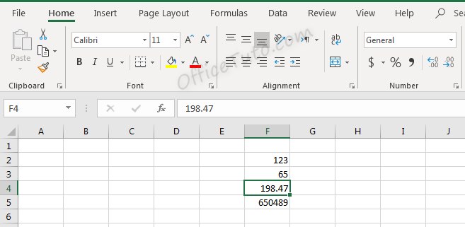
Note in the above screenshot that since we didn’t choose the “Number” format for our cells, they still have a “General” one. They are numbers for Excel (meaning, we can do calculations on them), but they didn’t have yet the number format and its formatting aspects:
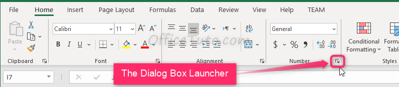
You can set the formatting options for Excel numbers in the “Format Cells” dialog box.
To do that, select the cell or the range of cells you want to set the formatting options for their numbers, and go to the “Home” tab of the ribbon, then in the “Number” group of commands, click on the launcher of the dialog box (the arrow on the right-down side of the group).
Excel opens the “Format Cells” dialog box in its “Number” tab. Click in the “Category” pane on “Number”.
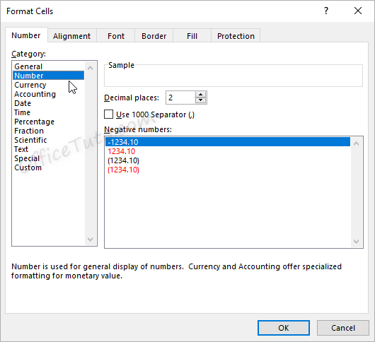
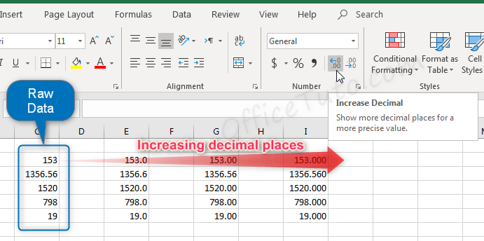
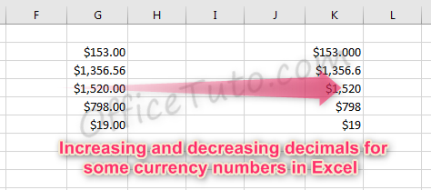
- In this dialog box, you can decide how many decimal places to display by updating options in the “Decimal places” field.
Note that this feature is also available in the “Home” tab of the ribbon where you can go to the “Number” group of commands and click the Increase Decimal ![]() or Decrease Decimal
or Decrease Decimal ![]() buttons.
buttons.
Here is the result of consecutive increasing of decimal places on our example of data (1 decimal; 2 decimals; and 3 decimals):
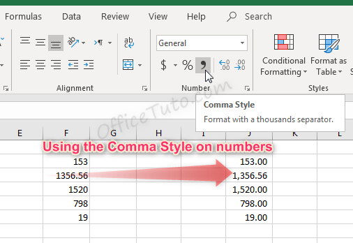
- You can also decide if commas should be shown in the display as a thousand separator, by updating the “Use 1000 Separator (,)” option in the “Format Cells” dialog box.
This feature is also available in the “Home” tab of the ribbon by clicking the “Comma Style” button ![]() in the “Number” group of commands.
in the “Number” group of commands.
Note that using the Comma Style button will automatically set the format to Accounting.
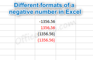
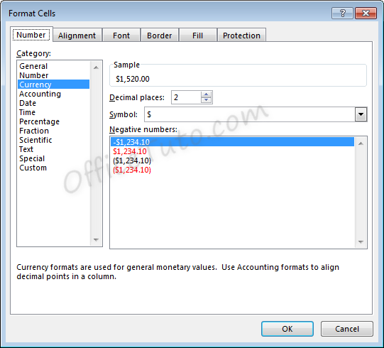
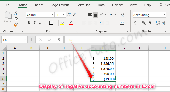
- Another option from the Format Cells dialog box is to decide how negative numbers should display by using the “Negative numbers” field.
There are four options for displaying negative
numbers.
- Display
negative numbers with a negative sign before the number. - Display
negative numbers in red. - Display
negative numbers in parentheses. - Display
negative numbers in red and in parentheses.
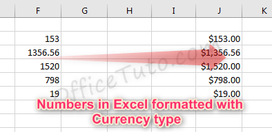
3- Currency format
Cells formatted as currency have a currency symbol such as a dollar sign $ immediately to the left of the number in the cell, and contain two numbers after the decimal by default.
The alignment of numbers in currency formatted cells will be on the right for readability.
Currency formatting options are similar to
number formatting options, apart from the currency symbol display.
- As with regular number formatting, you can decide, in the “Format Cells” dialog box, how many decimal places to display by updating the field “Decimal places”.
You can also find this feature in the “Home” tab of the ribbon, by going to the “Number” group of commands and clicking the Increase Decimal ![]() or Decrease Decimal
or Decrease Decimal ![]() .
.
- You can also decide what currency symbol should be shown in the display by updating the “Symbol” field in the “Format Cells” dialog box.
- As with regular number formatting, you can also decide how negative numbers should display by updating the “Negative numbers” field in the “Format Cells” dialog box.
There are four
options for displaying negative numbers.
- Display
negative numbers with a negative sign before the number. - Display
negative numbers in red. - Display
negative numbers in parentheses. - Display
negative numbers in red and in parentheses.
4- Accounting format
Like with the currency format, cells formatted as accounting have a currency symbol such as a dollar sign $; however, this symbol is to the far left of the cell, while the alignment of numbers in the cell is on the right. Accounting numbers contain two numbers after the decimal by default.
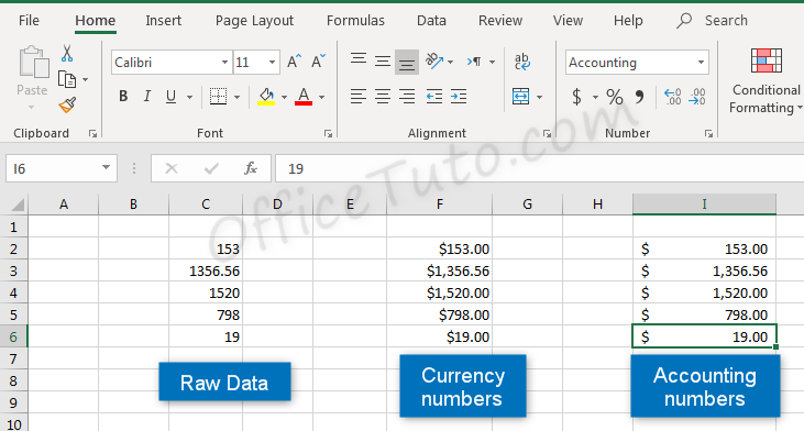
Clicking the “Accounting Number Format” button ![]() in the “Number” group of commands of the “Home” tab, will quickly format a cell or cells as Accounting.
in the “Number” group of commands of the “Home” tab, will quickly format a cell or cells as Accounting.
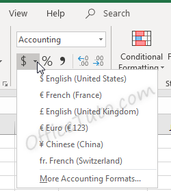
The down arrow to the right of the Accounting Number Format button allows selection between common symbols used for accounting, including English (dollar sign), English (pound), Euro, Chinese, and French symbols.
Accounting formatting options in the “Format Cells” dialog box (“Home” tab of the ribbon, in the “Number” group of commands, click on the launcher of the “Number Format” dialog box), are similar to number and currency formatting options.
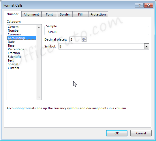
- You can decide how many decimal places to display by updating its option in the “Format Cells” dialog box.
As mentioned before in this tutorial, this feature is also available directly in the “Home” tab of the ribbon by clicking the Increase Decimal ![]() or Decrease Decimal
or Decrease Decimal ![]() buttons in the “Number” group of commands.
buttons in the “Number” group of commands.
- You can also decide in the “Format Cells” dialog box, what currency symbol should be shown in the display by using the “Symbol” drop-down list.
This dropdown gives a much broader list of options than the “Accounting Number Format” option in the “Home” tab of the ribbon.
Note that with the Accounting formatting option, negative numbers display in parentheses by default. There are not options to change this.
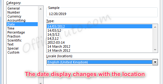
5- Date format
There are options for “Short Date” and “Long Date” in the “Number Format” dropdown list of the “Home” tab.
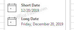
Short date shows the date with slashes separating month, day, and year. The order of the month and day may vary depending on your computer’s location settings.
Long date shows the date with the day of the week, month, day, and year separated by commas.
More options for formatting dates are available in the “Format Cells” dialog box (accessible by clicking in the “Number Format” dropdown list of the “Home” tab and choosing the “More Number Formats” option at the bottom).
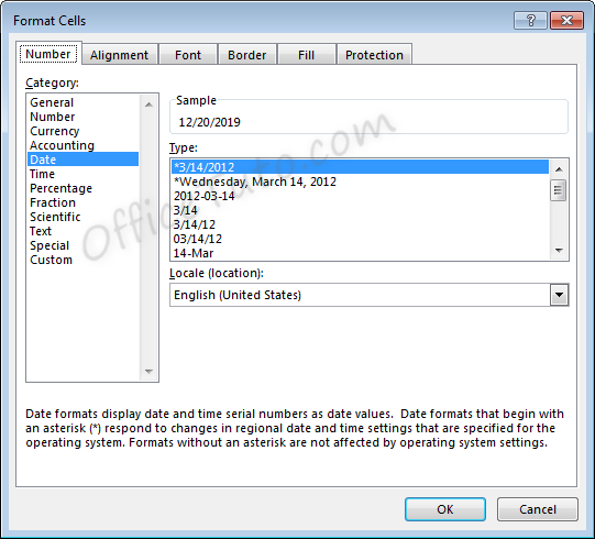
- You can choose from a long list of available date formats.
- You can update the location settings used for formatting the date. This will alter the list of format options in the above list and will adjust the display and potentially the order of the elements (day, month, year) within the date.
Note the below example when we switch from English (United States) format to English (United Kingdom) format.
6- Time format
Cells formatted as time display the time of
day. The default time display is based on your computer’s location settings.
Time formatting options are available in the “Format Cells” dialog box (accessible by choosing the “More Number Formats” option at the bottom of the “Number Format” dropdown list in the “Home” tab of the ribbon).
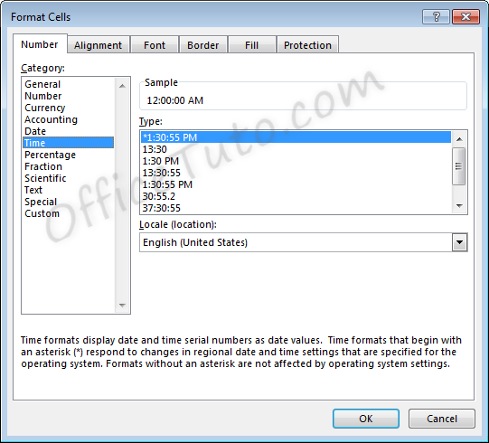
- You can choose from a long list of available time formats.
- You can update the location settings used for formatting the time. This will alter the list of format options in the above list and will adjust the display.
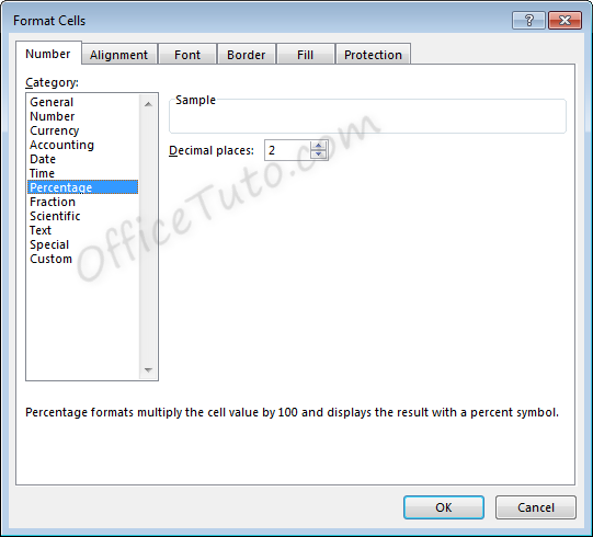
7- Percentage format
Cells formatted as percentage display a percent sign to the right of the number. You can change the format of a cell to a percentage using the “Number Format” dropdown list, or by clicking the “Percent Style” button ![]() . Both options are accessible from the “Home” tab of the ribbon, in the “Number” group of commands.
. Both options are accessible from the “Home” tab of the ribbon, in the “Number” group of commands.
Note that updating a number to a percentage
will expect that the number already contains the decimal. For example:
A cell containing the value 0.08, as a percentage, will show 8%.
A cell containing the value 8, as a percentage, will show 800%.
Percentage formatting options are available in the “Format Cells” dialog box, accessible by clicking on “More Number Formats” of the “Number Format” dropdown list in the “Home” tab of the ribbon.
8- Fraction format
Cells formatted as a fraction display with a slash
symbol separating the numerator and denominator.
Fraction formatting options are available in the “Format Cells” dialog box, accessible by clicking in the “Home” tab of the ribbon, on “More Number Formats” of the “Number Format” dropdown list.
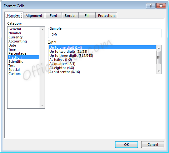
- Note that
when selecting the format to use for a fraction, Excel will round to the
nearest fraction where the formatting criteria can be met.
As an example, if the
formatting option selected is “Up to one digit”, entering a fraction with two
digits will cause rounding to occur. For example, with the setting of “Up to
one digit”,
If we enter a value of 7/16, the value displayed will be 4/9, as converting to 9ths was the option with only one digit which required the least amount of rounding.
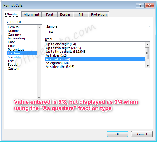
For another example, if the formatting option selected is “As quarters”, entering a fraction that cannot be expressed in quarters (divisible by four) will also cause rounding to occur.
If we enter a value of 5/8, the value displayed will be 3/4. Excel rounded up to 6/8, or 3/4, which was the closest option divisible by four.
- Also note
that for the formatting options with “Up to x digits”, Excel will always round
down to the lowest exact equivalent fraction when possible.
For example, if we enter a value of 2/4 with one of these formatting options active, the value displayed will be 1/2, as this is the mathematical equivalent. This behavior will not take place for formatting options “As…”, since these specifically determine what the denominator should be.
- Fractions listed as more than a whole (meaning the numerator is a higher number than the denominator), such as 7/4 will automatically be adjusted into a whole number and a fraction 13/4, where the fraction follows the formatting rules selected.
9- Scientific format
Scientific format, otherwise known as
Exponential Notation, allows very large and small numbers to be accurately
represented within a cell, even when the size of the cell cannot accommodate
the size of the numbers.
The way exponential notation works is to theoretically place a decimal in a spot that would make the number shorter, then describe where to move that decimal to return to the original number.
Examples with large numbers, where the decimal is moved to the left:
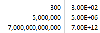
For the number 300 to be expressed in
exponential notation, Excel moves the decimal from after the whole number
300.00 to between the 3 and the 00. This is typed out as E+02 since the decimal
was moved two places to the left. The other examples are similar, where the
decimal was moved 6 and 12 places to the left.
Examples with small numbers, where the decimal is moved to the right:
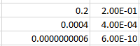
For the number 0.2 to be expressed in
exponential notation, Excel moves the decimal to create a whole number 2. This
is typed out as E-01 since the decimal was moved one place to the right. The
other examples are similar, where the decimal was moved 4 and 10 places to the
right.
Scientific formatting options are listed in the “Format Cells” dialog box, accessible by going to the “Home” tab of the ribbon, and clicking the “More Number Formats” option of the “Number Format” dropdown list.
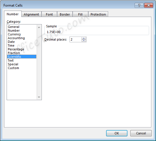
The only option available is to alter the
number of decimal places shown in the number prior to the scientific notation.
For example, for the value 11.43 formatted with the scientific format, if we change the Decimal places from 2 to 1, the display will change as follows.
Two decimals: 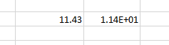
One decimal: 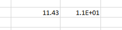
10- Text format
Cells can be formatted as Text through the
“Number Format” dropdown list, in the “Number” group of commands of the “Home”
tab.
Using the Text format in Excel allows values to be entered as they are, without Excel changing them per the above formatting rules.
In general, when entering a text in a cell, you won’t need to set its type to “Text”, as the default format type “General” is sufficient in most cases.
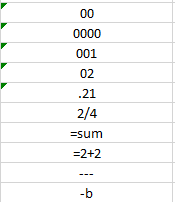
This may be useful when you want to display numbers with leading zeros, want to have spaces before or after numbers or letters, or when you want to display symbols that Excel normally uses for formulas.
Below are examples of some fields formatted as Text.
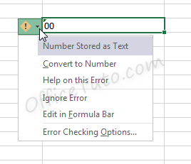
Note that when a number is formatted as Text, Excel will display a symbol showing that there could be a possible error ![]() .
.
Clicking the cell, then clicking the pop-up icon will show what the error may be and offer suggestions for resolution.
11- Special format
Special format offers four options in the “Format Cells” dialog box, accessible by going to the “Home” tab of the ribbon, and clicking the launcher arrow in the “Number” group of commands.
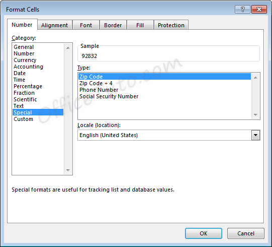
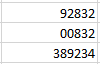
- Zip Code
When less than five numbers are entered in Zip
Code format, leading zeros will be added to bring the total to five numbers.
When more than five numbers are entered in Zip Code format, all numbers will be displayed, even though this does not meet the format criteria.
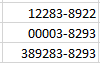
- Zip Code + 4
Zip Code + 4 format automatically creates a
dash symbol – before the last four numbers in the zip code.
When less than nine numbers are entered in Zip
Code + 4 format, leading zeros will be added to bring the total to nine
numbers.
When more than nine numbers are entered in Zip Code + 4 format, extra numbers are displayed prior to the dash symbol –.
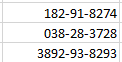
- Phone Number
Phone Number format automatically creates a
dash –
before the last four numbers in the phone number. This format also adds
parentheses ( ) around the area code when an area code is entered.
When less than the expected number of digits
are entered in Phone Number format, only the entered digits will be displayed,
starting from the end of the phone number, as shown on the third and fourth
lines, below.
When more than the expected number of digits
are entered in Phone Number format, extra numbers are displayed within the area
code parentheses.
Note that Phone Number format in Excel does not handle the number 1 before an area code. This entry would be treated like any other extra number.

- Social Security Number
Social Security Number format automatically
creates a dash – before the last four numbers in the social security number
and a dash before the last six numbers in the social security number.
When less than nine numbers are entered in
Social Security Number format, leading zeros will be added to bring the total
to nine numbers.
When more than nine numbers are entered in Social Security Number format, extra numbers are displayed prior to the first dash –.
12- Custom format
Custom formats can be used or added through the
“Format Cells” dialog box, accessible from the “Number” group of commands in
the “Home” tab of the ribbon by clicking the “Number Format” launcher arrow.
This can be useful if the above formatting options do not work for your needs. Custom number formats can be created or updated by typing into the “Type” field of the “Format Cells” dialog box.
When creating a new custom format, be sure to use an existing custom format that you are okay with changing.
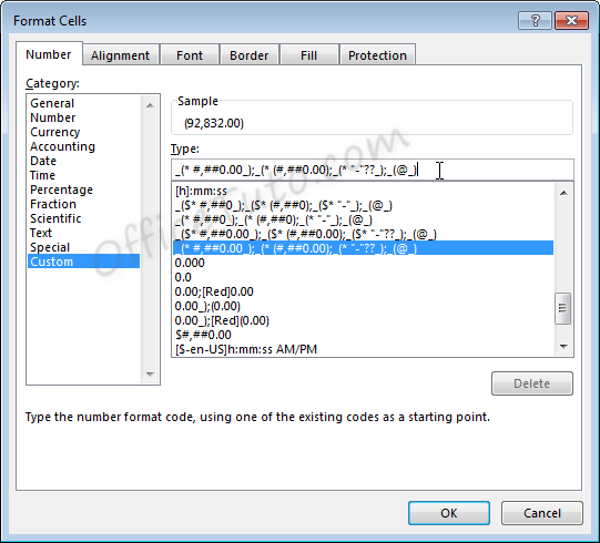
Custom number formats are separated, at
maximum, into four parts separated by semicolons ; .
- Part 1: How
to handle positive number values - Part 2: How
to handle negative number values - Part 3: How
to handle zero number values - Part 4: How
to handle text values
Note that if fewer parts are included in the custom format coding, Excel will determine how best to merge the above options: As an example, if two parts are listed, positive and zero values will be grouped.
Note that Excel may update the formatting of some fields to Custom automatically depending on what actions are taken on the field.
C- Common issues caused by wrong cell format types in Excel
1- Common issues due to wrong cell format types in Excel
The most common problems you may encounter with a wrong cell format type in Excel are of 3 types:
– Getting a wrong value.
– Getting an error.
– Formula displayed as-is and not calculated.
Let’s illustrate these 3 cases with some examples:
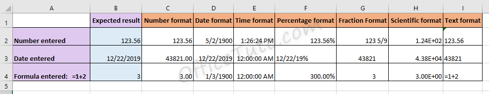
- Getting a wrong value
This may occur when you enter a value in an already formatted cell with an inappropriate format type, or when you apply a different format to a cell already containing a value.
The following table details some examples:
- Getting an error
This occurs when you enter a text preceded with a symbol of a dash, or plus, or equal, as an element of a list.
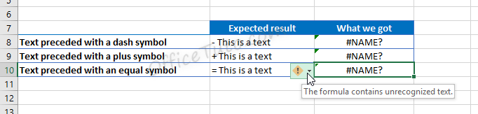
Excel wrongly interprets the text as a formula and show the error “The formula contains unrecognized text”.
- Formula displayed as-is and not calculated
In the following example, we tried to calculate the total of prices from cell B2 to B6 using the Excel SUM function, but Excel doesn’t calculate our formula and just displayed it as-is.
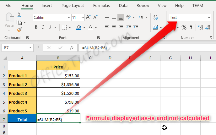
The source of the problem is that the result cell, B7, was previously formatted as text before entering the formula.
2- How to correct wrong cell format type issues in Excel
To correct cell format type issues in Excel, apply the right format in the “Number Format” drop-down list, and sometimes, you’ll also need to re-enter the content of the cell. For cells with formulas displayed as text, choose the “General” format, then double click in the cell and press Enter.

Jeff Golden is an experienced IT specialist and web publisher that has worked in the IT industry since 2010, with a focus on Office applications.
On this website, Jeff shares his insights and expertise on the different Office applications, especially Word and Excel.

In this lesson we discuss cell references, how to copy or move a formula, and format cells. To begin, let’s clarify what we mean by cell references, which underpin much of the power and versatility of formulas and functions. A concrete grasp on how cell references work will allow you to get the most out of your Excel spreadsheets!
Note: we’re just going to assume that you already know that a cell is one of the squares in the spreadsheet, arranged into columns and rows which are referenced by letters and numbers running horizontally and vertically.
What is a Cell Reference?
A “cell reference” means the cell to which another cell refers. For example, if in cell A1 you have =A2. Then A1 refers to A2.

Let’s review what we said in Lesson 2 about rows and columns so that we can explore cell references further.
Cells in the spreadsheet are referred to by rows and columns. Columns are vertical and labeled with letters. Rows are horizontal and labeled with numbers.
The first cell in the spreadsheet is A1, which means column A, row 1, B3 refers to the cell located on the second column, third row, and so on.
For learning purposes about cell references, we will at times write them as row, column, this is not valid notation in the spreadsheet and is simply meant to make things clearer.
Types of cell references
There are three types of cell references.
Absolute – This means the cell reference stays the same if you copy or move the cell to any other cell. This is done by anchoring the row and column, so it does not change when copied or moved.
Relative – Relative referencing means that the cell address changes as you copy or move it; i.e. the cell reference is relative to its location.
Mixed – This means you can choose to anchor either the row or the column when you copy or move the cell, so that one changes and the other does not. For example, you could anchor the row reference then move a cell down two rows and across four columns and the row reference stays the same. We will explain this further below.
Relative References
Let’s refer to that earlier example – suppose in cell A1 we have a formula that simply says =A2. That means Excel output in cell A1 whatever is inputted into cell A2. In cell A2 we have typed “A2” so Excel displays the value “A2” in cell A1.
Now, suppose we need to make room in our spreadsheet for more data. We need to add columns above and rows to the left, so we have to move the cell down and to the right to make room.
As you move the cell to the right, the column number increases. As you move it down, the row number increases. The cell that it points to, the cell reference, changes as well. This is illustrated below:
Continuing with our example, and looking at the graphic below, if you copy the contents of cell A1 two to the right and four down you have moved it to cell C5.
We copied the cell two columns to the right and four down. This means we have changed the cell it refers two across and four down. A1=A2 now is C5=C6. Instead of referring to A2, now cell C5 refers to cell C6.
The value shown is 0 because cell C6 is empty. In cell C6 we type “I am C6” and now C5 displays “I am C6.”
Example: Text Formula
Let’s try another example. Remember from Lesson 2 where we had to split a full name into first and last name? What happens when we copy this formula?
Write the formula =RIGHT(A3,LEN(A3) – FIND(“,”,A3) – 1) or copy the text to cell C3. Do not copy the actual cell, only the text, copy the text, otherwise it will update the reference.
You can edit the contents of a cell at the top of a spreadsheet in the box next to where is says “fx.” That box is longer than a cell is wide, so it is easier to edit.
Now we have:
Nothing complicated, we have just written a new formula into cell C3. Now copy C3 to cells C2 and C4. Observe the results below:
Now we have Alexander Hamilton and Thomas Jefferson’s first names.
Use the cursor to highlight cells C2, C3, and C4. Point the cursor to cell B2 and paste the contents. Look at what happened – we get an error: “#REF.” Why is this?
When we copied the cells from column C to column B it updated the reference one column to the left =RIGHT(A2,LEN(A2) – FIND(“,”,A2) – 1).
It changed every reference to A2 to the column to the left of A, but there is no column to the left of column A. So the computer does not know what you mean.
The new formula in B2 for example, is =RIGHT(#REF!,LEN(#REF!) – FIND(“,”,#REF!) – 1) and the result is #REF:
Copying a Formula to a Range of Cells
Copying cells is very handy because you can write one formula and copy it to a large area and the reference is updated. This avoids having to edit each cell to ensure it points to the correct place.
By “range” we mean more than one cell. For example, (C1:C10) means all the cells from cell C1 to cell C10. So it is a column of cells. Another example (A1:AZ1) is the top row from column A to column AZ.
If a range cross five columns and ten rows, then you indicate the range by writing the top-left cell and bottom right one, e.g., A1:E10. This is a square area that cross rows and columns and not just part of a column or part of a row.
Here is an example that illustrates how to copy one cell to multiple locations. Suppose we want to show our projected expenses for the month in a spreadsheet so we can make a budget. We make a spreadsheet like this:
Now copy the formula in cell C3 (=B3+C2) to the rest of the column to give a running balance for our budget. Excel updates the cell reference as you copy it. The result is shown below:
As you can see, each new cell updates relative to the new location, so cell C4 updates its formula to =B4 + C3:
Cell C5 updates to =B5 + C4, and so on:
Absolute References
An absolute reference does not change when you move or copy a cell. We use the $ sign to make an absolute reference – to remember that, think of a dollar sign as an anchor.
For example, enter the formula =$A$1 in any cell. The $ in front of the column A means do not change the column, the $ in front of the row 1 means do not change the column when you copy or move the cell to any other cell.
As you can see in the example below, in cell B1 we have a relative reference =A1.When we copy B1 to the four cells below it, the relative reference =A1 changes to the cell to the left, so B2 become A2, B3 become A3, etc. Those cells obviously have no value inputted, so the output is zero.
However, if we use =$A1$1, such as in C1 and we copy it to the four cells below it, the reference is absolute, thus it never changes and the output is always equal to the value in cell A1.
Suppose you are keeping track of your interest, such as in the example below. The formula in C4 = B4 * B1 is the “interest rate” * “balance” = “interest per year.”
Now, you have changed your budget and have saved an additional $2,000 to buy a mutual fund. Suppose it is a fixed rate fund and it pays the same interest rate. Enter the new account and balance into the spreadsheet and then copy the formula = B4 * B1 from cell C4 to cell C5.
The new budget looks like this:
The new mutual fund earns $0 in interest per year, which can’t be right since the interest rate is clearly 5 percent.
Excel highlights the cells to which a formula references. You can see above that the reference to the interest rate (B1) is moved to the empty cell B2. We should have made the reference to B1 absolute by writing $B$1 using the dollars sign to anchor the row and column reference.
Rewrite the first calculation in C4 to read =B4 * $B$1 as shown below:
Then copy that formula from C4 to C5. The spreadsheet now looks like this:
Since we copied the formula one cell down, i.e. increased the row by one, the new formula is =B5*$B$1. The mutual fund interest rate is calculated correctly now, because the interest rate is anchored to cell B1.
This is a good example of when you could use a “name” to refer to a cell. A name is an absolute reference. For example, to assign the name “interest rate” to cell B1, right-click the cell and then select “define name.”
Names can refer to one cell or a range, and you can use a name in a formula, for example =interest_rate * 8 is the same thing as writing =$B$1 * 8.
Mixed References
Mixed references are when either the row or column is anchored.
For example, suppose you are a farmer making a budget. You also own a feed store and sell seeds. You are going to plant corn, soybeans, and alfalfa. The spreadsheet below shows the cost per acre. The “cost per acre” = “price per pound” * “pounds of seeds per acre” – that’s what it will cost you to plant an acre.
Enter the cost per acre as =$B2 * C2 in cell D2. You are saying you want to anchor the price per pound column. Then copy that formula to the other rows in the same column:
Now you want to know the value of your inventory of seeds. You need the price per pound and the number of pounds in inventory to know the value of the inventory.
We add two columns: “pound of seed in inventory” and then “value of inventory.” Now, copy the cell D2 to F4 and note that the row reference in the first part of the original formula ($B2) is updated to row 4 but the column remains fixed because the $ anchors it to “B.”
This is a mixed reference because the column is absolute and the row is relative.
Circular References
A circular reference is when a formula refers to itself.
For example, you cannot write c3 = c3 + 1. This kind of calculation is called “iteration” meaning it repeats itself. Excel does not support iteration because it calculates everything only one time.
If you try do this by typing SUM(B1:B5) in cell B5:
A warning screen pops up:
Excel only tells you that you have a circular reference at the bottom of the screen so you might not notice it. If you do have a circular reference and close a spreadsheet and open it again, Excel will tell you in a pop-up window that you have a circular reference.
If you do have a circular reference, every time you open the spreadsheet, Excel will tell you with that pop-up window that you have a circular reference.
References to Other Worksheets
A “workbook” is a collection of “worksheets.” Simply put, this means you can have multiple spreadsheets (worksheets) in the same Excel file (workbook). As you can see in the example below, our example workbook has many worksheets (in red).
Worksheets by default are named Sheet1, Sheet2, and so forth. You create a new one by clicking the “+” at the bottom of the Excel screen.
You can change the worksheet name to something useful like “loan” or “budget” by right-clicking on the worksheet tab shown at the bottom of the Excel program screen, selecting rename, and typing in a new name.
Or you can simply double-click on the tab and rename it.
The syntax for a worksheet reference is =worksheet!cell. You can use this kind of reference when the same value is used in two worksheets, examples of that might be:
- Today’s date
- Currency conversion rate from Dollars to Euros
- Anything that is relevant to all the worksheets in the workbook
Below is an example of worksheet “interest” making reference to worksheet “loan,” cell B1.
If we look at the “loan” worksheet, we can see the reference to the loan amount:
Coming up Next …
We hope you now have a firm grasp of cell references including relative, absolute, and mixed. There’s certainly a lot.
That’s it for today’s lesson, in Lesson 4, we will discuss some useful functions you may wish to know for daily Excel use.
READ NEXT
- › How to Adjust and Change Discord Fonts
- › This New Google TV Streaming Device Costs Just $20
- › Google Chrome Is Getting Faster
- › HoloLens Now Has Windows 11 and Incredible 3D Ink Features
- › The New NVIDIA GeForce RTX 4070 Is Like an RTX 3080 for $599
- › BLUETTI Slashed Hundreds off Its Best Power Stations for Easter Sale
There are several ways to color format cells in Excel, but not all of them accomplish the same thing. If you want to fill a cell with color based on a condition, you will need to use the Conditional Formatting feature.
Fill a cell with color based on a condition
Before learning to conditionally format cells with color, here is how you can add color to any cell in Excel.
Cell static format for colors
You can change the color of cells by going into the formatting of the cell and then go into the Fill section and then select the intended color to fill the cell.

In the above example, the color of cell E3 has been changed from No Fill to Blue color, and notice that the value in cell E3 is 6 and if we change the value in this cell from 6 to any other value the cell color will not change and it will always remain blue. What does this mean?
This means that cell color is independent of cell value, so no matter what value will be in E3 the cell color will always be blue. We can refer to this as static formatting of the cell E3.
Conditional formatting cell color based on cell value
Now, what if we want to change the cell color based on cell value? Suppose we want the color of cell E3 to change with the change of the value in it. Say, we want to color code the cell E3 as follows:
- 0-10 : We want the cell color to be Blue
- 11-20 : We want the cell color to be Red
- 21-30 : We want the cell color to be Yellow
- Any other value or Blank : No color or No Fill.
We can achieve this with the help of Conditional Formatting. On the Home tab, in the Style subgroup, click on Conditional Formatting→New Rule.
Note: Make sure the cell on which you want to apply conditional formatting is selected

Then select “Format only cells that contain,” then in the first drop down select “Cell Value” and in the second drop-down select “between” :

Then, on the first box, enter 0 and in the second box, enter 10, then click on the Format button and go to Fill Tab, select the blue color, click Ok and again click Ok. Now enter a value between 0 and 10 in cell E3 and you will see that cell color changes to blue and if there is any other value or no value then cell color revert to transparent.

Repeat the same process for 11-20 and 21-30 and you’ll see that number changes as per the value of the cell.
Conditional formatting with text
Similarly, we can do the same process for text values as well instead of numerical values by using the “Specific Text” in the first drop down and in the second drop-down select either of 4 values containing, not containing, beginning with, ending with and then enter the specific text in the text box.
For Example:
First, select the cell on which you want to apply conditional format, here we need to select cell B1. On the home tab, in the Styles subgroup, click on Conditional Formatting→New Rule.
Now select Format only cells that contain the option, then in the first drop down select “Specific Text” and in the second drop-down select either of the 4 options: containing, not containing, beginning with, ending with. In the example below, we use beginning with “J” and then select Format button to select Blue as the fill color.

Conditional format based on another cell value
In the example above, we are changing the cell color based on that cell value only, we can also change the cell color based on other cells value as well. Suppose we want to change the color of cell E3 based on the value in D3, to do that we have to use a formula in conditional formatting.
Now suppose if we want to change cell E3 color to blue if the D3 value is greater than 3 and to green if the D3 value is greater than 5 and to red, if D3’s value is greater than 10, we can do that with the conditional format using a formula.
Again follow the same procedure.
First, select the cell on which you want to apply conditional format, here we need to select cell E3. On the home tab, in the Styles subgroup, click on Conditional Formatting→New Rule.
Now select Use a formula to determine which cells to format option, and in the box type the formula: D3>5; then select Format button to select green as the fill color.

Keep in mind that we are changing the format of cell E3 based on cell D3 value, note that the cursor now is pointing at E3, which is the cell we use to set conditional format. The formula “=D3>5” means if D3 is greater than 5 then the value of E3 will change to green. Click ok and see the color of cell E3 changes to green as D3 right now contains 6.

Now let’s apply the conditional formatting to E3 if D3 is greater than 3. This means if D3>3 then cell color should become “Blue” and if D3>5 then cell color should remain green as we did it in the previous step.
Now, if you follow the above steps as we did for Green color, you will see that even if the cell value is 6, it is showing blue color and not green, because it takes the latest conditional formatting we set for that cell, and as 6 is also greater than 3 hence it is showing blue color but it should show green color.
So, we have to arrange the rules we have applied for any particular cells, we can do that by going into Manage Rules option of conditional formatting.

You can see all the rules applied to that cell and then we can arrange the rules or set their priority by using the arrow buttons. A number greater than 5 will also be greater than 3, hence greater than 5 rule will take higher priority and we can move it upward using the arrow buttons.


Now when you enter 6 in D3, the cell color of E3 will become green and when you enter 4, the cell color will become blue.
If you are tired of reading too many articles without finding your answer or need a real Expert to help you save hours of struggle, click on this link to enter your problem and get connected to a qualified Excel expert in a few seconds. You can share your file and an expert will create a solution for you on the spot during a 1:1 live chat session. Each session last less than 1 hour and the first session is free.
Are you still looking for help with Conditional Formatting? View our comprehensive round-up of Conditional Formatting tutorials here.
The best part of conditional formatting is you can use formulas in it. And, it has a very simple sense to work with formulas.
Your formula should be a logical formula and the result should be TRUE or FALSE. If the formula returns TRUE, you’ll get the formatting, and if FALSE then nothing. The point is, by using formulas you can make the best out of conditional formatting.
Yes, that’s right. In the below example, we have used a formula in CF to check whether the value in the cell is smaller than 1000 or not.

And if that value is smaller than 1000 it will apply the formatting which we have specified, otherwise not. So today in this post, I’d like to share with you simple steps to apply conditional formatting using a formula. And some of the useful examples that you can use in your daily work.
Steps to Apply Conditional Formatting with Formulas
The steps to apply CF with formulas are quite simple:
- Select the range to apply Conditional Formatting.
- Add a formula to text a condition.
- Specify a format to apply when the condition is met.

To learn this in a proper way make sure to download this sample file from here and follow the below-detailed steps.
- First of all, select the range where you want to apply conditional formatting.

- After that, go to Home Tab ➜ Styles ➜ Conditional Formatting ➜ New Rule ➜ Use a formula to determine which cell to format.

- Now, in the “Format values where formula is true” enter the below formula.
=E5<1000

- The next thing is to specify the format to apply and for this, click on the format button and select the format.

- In the end, click OK.
While entering a formula in the CF dialog box you can’t see its result or whether that formula is valid or not. So, the best practice is to check that formula before using it in CF by entering it in a cell.
1. Use a Formula that is Based on Another Cell
Yes, you can apply conditional formatting based on another cell’s value. If you look at the below example, we have added a simple formula that is based on another cell. And if the value of that linked cell meets the condition specified, you’ll get conditional formatting.

When achievement will be below 75%, it will highlight in red color.

2. Conditional Formatting using IF
Whenever I think about conditions, the first thing that comes to my mind is using the IF function. And the best part of this function is, that it fits perfectly in conditional formatting. Let me show you an example:

Here, we have used the IF to create a condition and the condition is when the count of “Done” in range B3:B9 is equal to the count of tasks in the range A3:A9, then the final status will appear.
2. Conditional Formatting with Multiple Conditions
You can create multiple checks in conditions to apply to the format. Once all the conditions or one of the conditions will meet, conditional formatting will apply to the cell. Look at the below example where we have used the average temperature of my town.
And we have used a simply combined IF-AND to highlight the months when the temperature is pretty pleasant. Months where the temperature is between 15 Celsius to 35 Celsius, will get colored.
Just like this, you can also use if with or function.
4. Highlight Alternate Rows with Conditional Formatting
To highlight every alternate row you can use the following formula n CF.
=INT(MOD(ROW(),2))
By using this formula, every row whose number is odd will be highlighted. And, if you want to do vice versa you can use the following formula.

=INT(MOD(ROW()+1,2))
The same kind of formula can use for columns (odd and even) as well.
=INT(MOD(COLUMN(),2))
And for even columns.
=INT(MOD(COLUMN()+1,2))
5. Highlight Cells with Errors using CF
Now let’s come to another example where we will check whether a cell contains an error or not. What we need to do is just insert a formula in conditional formatting that can check the condition and return the result in TRUE or FALSE. You can even verify cells for numbers, text, or some specific values as well.

6. Create a Checklist with Conditional Formatting
Now let’s add some creativity to intelligence. You have already learned how to use a formula that is based on another cell. Here we have linked a checkbox with the B1 cell and further linked the B1 with the formula used in conditional formatting for cell A1.

Now, if you tick mark the checkbox, the value of cell B1 will turn into TRUE and cell A1 gets it conditional formatting [strikethrough].
Points to Remember
- Your formula should be a logical formula, which leads to a result as TRUE or FALSE.
- Try not to overload your data with conditional formatting.
- Always use relative and absolute references in a proper sense.
Sample File
Download this sample file from here to learn more.
More Tutorials
- AUTO FORMAT Option in Excel
- Apply Accounting Number Format in Excel
- Apply Background Color to a Cell or the Entire Sheet in Excel
- Print Excel Gridlines
- Add Page Number in Excel
- Apply Comma Style in Excel
- Apply Strikethrough in Excel
- Highlight Blank Cells in Excel
- Make Negative Numbers Red in Excel
- Cell Style (Title, Calculation, Total, Headings…) in Excel
- Change Date Format in Excel
- Highlight Alternate Rows in Excel with Color Shade
- Use Icon Sets in Excel (Conditional Formatting)
- Add Border in Excel
- Change Border Color in Excel
- Clear Formatting in Excel
- Copy Formatting in Excel
- Best Fonts for Microsoft Excel
- Hide Zero Values in Excel
⇠ Back to Advanced Excel Tutorials
This tutorial demonstrates how to apply conditional formatting based on a formula in Excel and Google Sheets.
Conditional Formatting in Excel comes with plenty of preset rules to enable you to quickly format cells according to their content. These preset rules do, however, have limitations, which is where using a formula to determine the format of a cell comes into play. This gives you much greater flexibility over your conditional formatting.
Conditional Formatting Formula Rules
Equal To
- Highlight the cells where you want to set the conditional formatting and then, in the Ribbon, select Home > Conditional Formatting > New Rule.
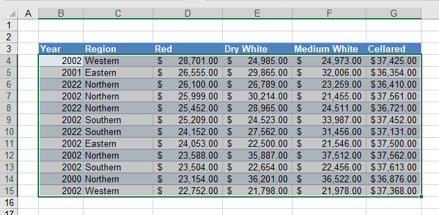
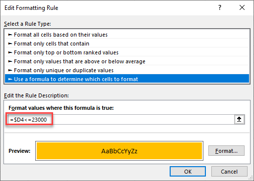
- Select Use a formula to determine which cells to format, and enter the formula:
=$C4=”Western”
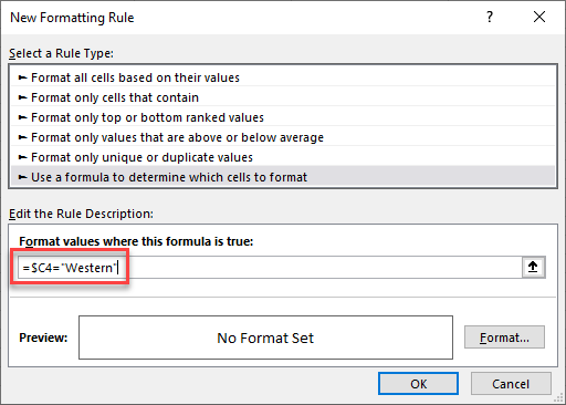
You always need to start your formula with an equal sign.
The formula tests whether the result is TRUE or FALSE much like the traditional Excel IF statement, but in the case of conditional formatting, you do not need to add the true and false conditions. If the formula returns TRUE, then formatting you set in the Format part of the rule is applied to the relevant cells.
You need to use a mixed reference in this formula ($C4) in order to lock the column (make it absolute) but make the row relative. This enables the formatting to format the entire row instead of just a single cell that meets the criteria.
When the rule is evaluated for all the cells in the range, the row changes, but the column does not. This causes the rule to ignore the values in any of the other columns and just concentrate on the values in Column C. If Column C of that row contains the word Western, the formula result is TRUE, and the formatting is applied for the whole row.
- Click Format… and select your desired formatting.
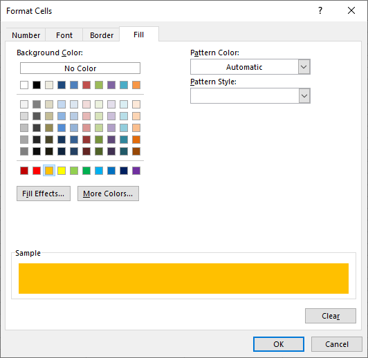
- Click OK and then OK again to view the result.
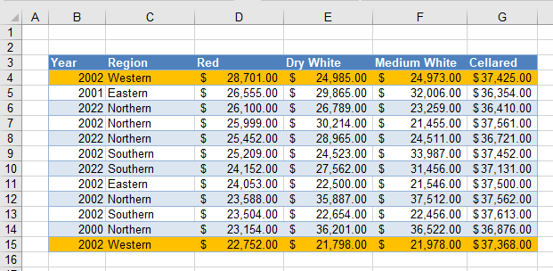
The rows where Column C is Western are highlighted, while other rows are not. In the example above, just two rows end up highlighted.
Not Equal
If you want to create an opposite rule, you can use the <> (not equal to) operator instead of =.
=$C4<>”Western”
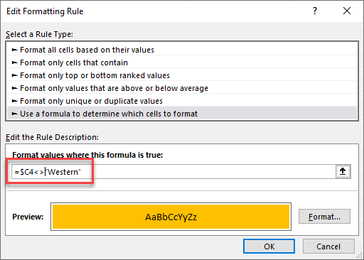
This results in the opposite: Most of the rows are now highlighted!
Greater Than
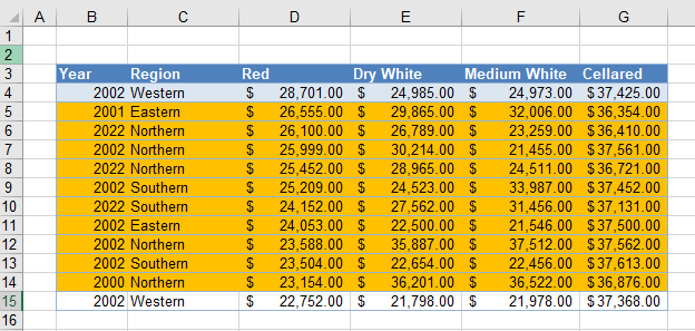
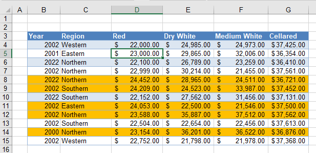
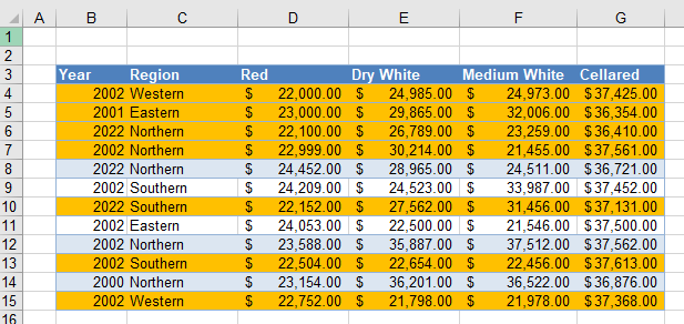
You can also test for greater than using a formula. For example, you can use a formula to check if the values in Column D are greater than $23,000.
=$D4>23000
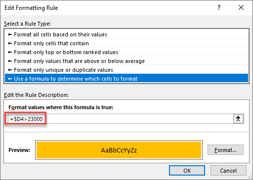
This rule highlights only rows where the value in Column D is greater than $23,000.
Greater Than or Equal To
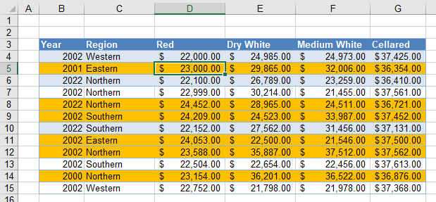
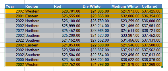
Similarly, you could highlight the rows where the value in Column D is greater than or equal to $23,000 with this formula below:
=$D4>=23000

The result for this formula would be slightly different: Rows where the Red value is exactly $23,000 are also highlighted (here, Row 5).
Less Than
Swapping the > sign for a < sign tests for values that are less than $23,000.
=$D4<23000

Now only rows where Red is less than $23,000 are highlighted.
Less Than or Equal To
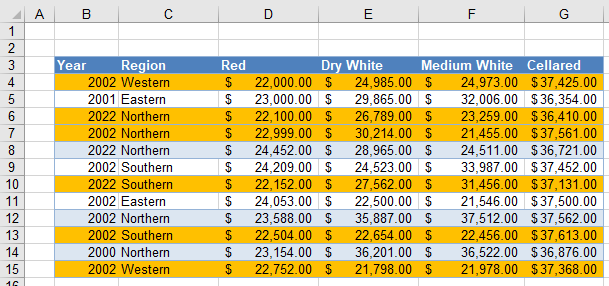
To change the test to include the target value (e.g., $23,000), use <=.
=$D4<=23000
Now, any rows in which Column D is equal to $23,000 are also highlighted.
Create Rules With OR, AND
OR Formula
You can create a more complicated rule by incorporating the Excel OR Function to expand the formula to look for two or more values.
- Enter the formula:
=OR($C4=”Western”,$C4=”Eastern”)
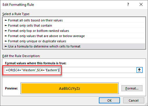
- Click on the Format… button and select your desired formatting, and then click OK to return to Excel.
This highlights all rows where the Region is Western or Eastern.
AND Formula
Similarly, you can create a rule using AND. This would mean checking the values in two or more columns.
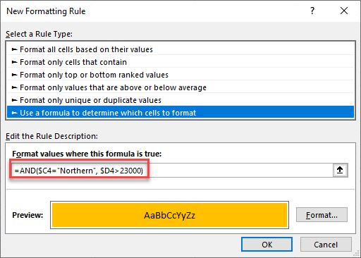
The formula above checks whether the text in Column C is Northern and the value in the corresponding row in Column D is greater than $23,000.
This conditional formatting rule highlights only the rows where both conditions are met.
IF Formula
You do not necessarily have to add an IF statement to the formula when you are creating it in a conditional formatting rule as the conditional formatting is always going to apply the rule if the formula that you have created returns a true value.
So, for example, this formula:
=IF($C4=”Western”,TRUE,FALSE)
and this formula
$C4=”Western”
both apply the same conditional formatting to your worksheet.
Built-in Excel Functions
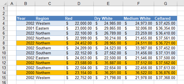
Many built-in Excel functions can be used in conditional formatting such as ISBLANK, ISERROR, ISEVEN, ISNUMBER, etc.
ISBLANK Function
You can use the ISBLANK Function to create a rule to find rows that contain blank or empty cells in the worksheet.
- Highlight the range and then, in the Ribbon, select Home > Conditional Formatting > New Rule.
- Type in the formula:
=ISBLANK($E3)
- Click on the Format… button and select your desired formatting and then click OK to return to Excel.
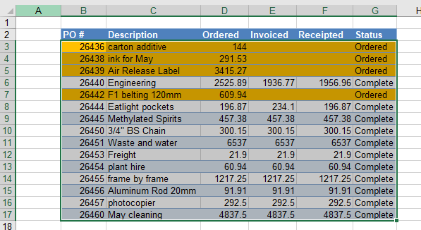
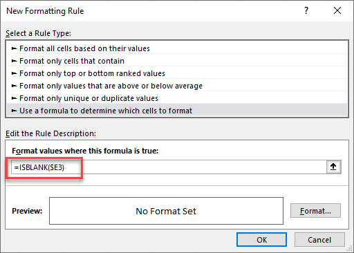
ISBLANK With OR
You can expand this to include blank cells or cells with an error in them.
- Type in the formula
=OR(ISBLANK($E3),ISERROR($E3))
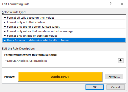
- Click on the Format… button and select your desired formatting and then click OK to return to Excel.
Other Functions in Conditional Formatting
There are a variety of other functions that can be used in creating conditional formatting formula-based rules.
- COUNTIFS – counts cells that meet a certain condition (useful for highlighting duplicates)
- LARGE – finds the kth largest value
- MAX – finds the largest number
- MIN – finds the smallest number
- MOD – returns the remainder after division (useful for highlighting every other row)
- NOT – changes TRUE to FALSE and vice versa
- NOW – returns the current date and time (useful for conditionally formatting dates and times)
- ROW – returns the number of rows in an array
- SEARCH – searches for a string of text within another string (useful for finding specific text)
- TODAY – returns the current date (useful for applying conditional formatting to dates)
- VLOOKUP – returns the result of a vertical lookup
- WEEKDAY – returns the day of the week
- XLOOKUP – a new, more powerful lookup function
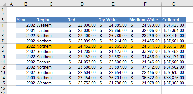
For example, you can use the MAX Function to highlight the row that contains the maximum value in a specified column.
=$D4=MAX($D:$D)
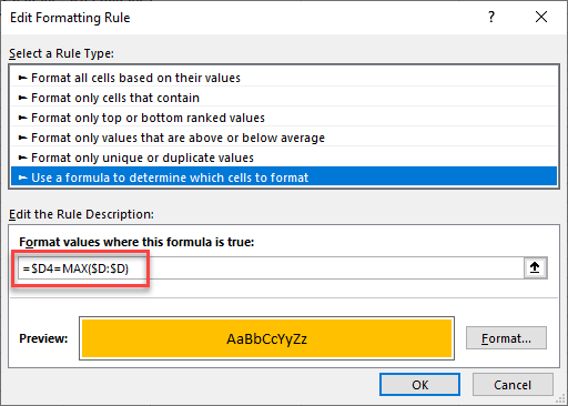
Now, only the row with the maximum value in Column D is highlighted.
If you are struggling to get a formula to work when creating a conditional formatting rule, it is a good idea to test the formula first in your Excel sheet. Once you have it right there, you can incorporate it in your rule.
Conditional Formatting Based on Formula in Google Sheets
Conditional Formatting works much the same in Google Sheets as it does in Excel.
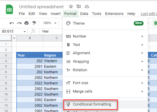
- Highlight the cells where you want to set the conditional formatting and then, in the Menu, select Format > Conditional formatting.
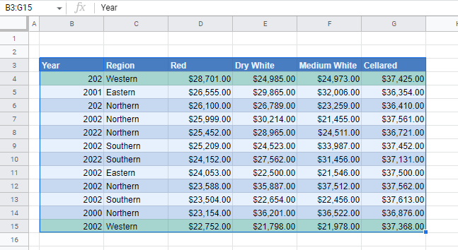
- Make sure the Apply to range is correct, and then select Custom formula is from the Format rules drop-down box. Type in the formula.
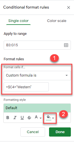
- Then, select your formatting style and click Done.
You can also use greater than, greater than or equal to, less than, and less than or equal to in Google Sheets.
AND and OR also work, as well the other functions listed above for Excel (except for XLOOKUP, which does not exist in Google Sheets).