
Excel for Microsoft 365 Excel for Microsoft 365 for Mac Excel 2021 Excel 2021 for Mac Excel 2019 Excel 2019 for Mac Excel 2016 Excel 2016 for Mac Excel 2013 Excel 2010 Excel 2007 Excel for Mac 2011 More…Less
Sometimes you need to check if a cell is blank, generally because you might not want a formula to display a result without input.

In this case we’re using IF with the ISBLANK function:
-
=IF(ISBLANK(D2),»Blank»,»Not Blank»)
Which says IF(D2 is blank, then return «Blank», otherwise return «Not Blank»). You could just as easily use your own formula for the «Not Blank» condition as well. In the next example we’re using «» instead of ISBLANK. The «» essentially means «nothing».
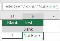
=IF(D3=»»,»Blank»,»Not Blank»)
This formula says IF(D3 is nothing, then return «Blank», otherwise «Not Blank»). Here is an example of a very common method of using «» to prevent a formula from calculating if a dependent cell is blank:
-
=IF(D3=»»,»»,YourFormula())
IF(D3 is nothing, then return nothing, otherwise calculate your formula).
Need more help?
Want more options?
Explore subscription benefits, browse training courses, learn how to secure your device, and more.
Communities help you ask and answer questions, give feedback, and hear from experts with rich knowledge.
We can use the conditional formatting approach for “cells that do not contain any value or for blank cells”. This step by step tutorial will assist all levels of Excel users on how to apply conditional formatting to blank cells.
Apply conditional formatting to blank cells
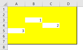
The aim of this exercise is apply formatting to the cells in Excel that are blank. For example, in Figure 1, the final result is to have all of the blank cells highlighted yellow. Here is how you can accomplish this:

Figure 1 – Final result
Setting up the Data
- First, we will set up our data by inputting the values for the items in the cells we choose.
- Our data is shown below.
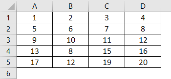
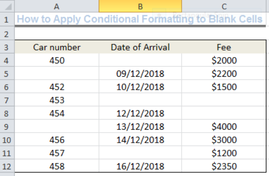 Figure 2- Setting up the Data
How to Apply Conditional Formatting To Blank Cells Only
We can see from our data in Figure 1 that the following cells are blank:
- A5 , A9, B4, B7, B11, C7 and C8
We can apply conditional formatting to all of these blank cells to show certain colors, patterns, etc. We can do this by following the simple steps outlined below.
- First, we have to select the data range of interest. The data range is from Cell A4 to Cell C12.
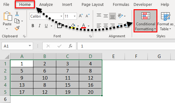
- Next, we have to click on conditional formatting as shown in figure 2 and click on the drop-down arrow.
![]() Figure 3- How to Apply Conditional Formatting for Only Blank Cells
Figure 3- How to Apply Conditional Formatting for Only Blank Cells
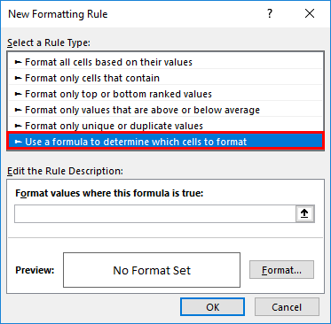
After we have clicked on the drop-down arrow, we will see a New Rule. Click on the New Rule and a dialog box called New formatting Rule will show up as shown in Figure 3.
![]() Figure 4- How to Apply Conditional Formatting for Only Blank Cells
Figure 4- How to Apply Conditional Formatting for Only Blank Cells
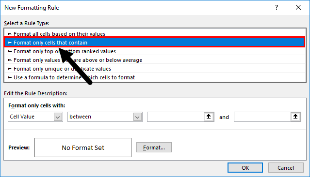
- Where you see Select a Rule Type as shown in Figure 3, click on Format only cells that contain.
- We also need to change the Rule Description to format only cells with blanks by clicking the drop-down arrow.
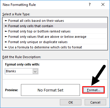
- We can use a range of conditional formatting options for the blank cells by clicking on Format adjacent to the No Format Set. For this example, let us use the Yellow color to fill cells that are blank. We will click on OK after selecting our choice.
![]() Figure 5- How to Apply Conditional Formatting for Only Blank Cells
Figure 5- How to Apply Conditional Formatting for Only Blank Cells
As we can see from Figure 5, all of the blank cells are now conditionally formatted in Yellow color.
![]() Figure 6- Output Showing the Result of Conditionally Formatted Blank Cells
Figure 6- Output Showing the Result of Conditionally Formatted Blank Cells
How to Apply Conditional Formatting Using a Custom Formula
- Syntax
=ISBLANK(VALUE)
- Syntax
=LEN(VALUE)
Explanation of formulas
A blank cell can contain a character such as space (just like the spaces we give when typing). We will type a space character into one of the blank cells (Cell A9).
The ISBLANK function returns as TRUE when a cell doesn’t contain “anything” and as FALSE when a cell contains at least one character.
The LEN function returns as TRUE for blank cells without any character and FALSE for cells with a character.
When using a custom formula for conditional formatting, it is essential that we enter the formula relative to the active cell in the selection. In this case, the cell is Cell A4. This will automatically update across the range where conditional formatting is intended to be applied.
Still applying the steps above, in figure 3, we will click on Use a formula to determine which cells to format.
 Figure 7- How to Use a Custom Formula for Conditional Formatting
We will click on OK afterward with the result being Figure 7. Remember that Cell A9 IS NO LONGER EMPTY BUT CONTAINS A SPACE CHARACTER.
Figure 8 – Output Showing the Result of Conditional Formatting with a Custom Formula
Using the same approach, we can input this string =LEN(A4)=0 into the Rule Description of figure 6 and we will arrive with the same result as figure 7.
How to Conditionally Format a Column Based on the Result from another Column
We can conditionally format the car number column based on the presence of a blank or visually empty cell (cell with at least a character). Cell A9 is visually empty because it has a space character. To do this, we can use the string below:
=$B4=””
We will select the car number column range (Cell A4 to Cell A12), follow the same procedure, and just like figure 6, we will input the string.
=$B4=””
The result in Figure 8 shows that cells in Column A have been conditionally formatted if they have corresponding cells on Column B (Date of Arrival) that are blank.
![]() Figure 9- Output of Conditional Formatting Based on the Blank Cells in Column B
Figure 9- Output of Conditional Formatting Based on the Blank Cells in Column B
If you are having any difficulty applying this, we have experts who are willing to help.
Are you still looking for help with Conditional Formatting? View our comprehensive round-up of Conditional Formatting tutorials here.
The logical expression =»» means «is empty». In the example shown, column D contains a date if a task has been completed. In column E, a formula checks for blank cells in column D. If a cell is blank, the result is a status of «Open». If the cell contains value (a date in this case, but it could be any value) the formula returns «Closed».
The effect of showing «Closed» in light gray is accomplished with a conditional formatting rule.
Display nothing if cell is blank
To display nothing if a cell is blank, you can replace the «value if false» argument in the IF function with an empty string («») like this:
=IF(D5="","","Closed")
Alternative with ISBLANK
Excel contains a function made to test for blank cells called ISBLANK. To use the ISBLANK, you can revise the formula as follows:
=IF(ISBLANK(D5),"Open","Closed")
You may want to find and highlight all blank cells in a range or sheet within your Excel® file.
You can use conditional formatting to highlight if a cell is blank. And you can also use conditional formatting to highlight any of these cell attributes:
- Is text
- Is a formula
- Is a constant
- Is an error
- The number of characters
- Is protected
If you only need to do a one-off test for blanks or the other attributes above within your range then skip down to ‘One-off cell attribute tests’. This will be quicker than adding conditional formats for this type of query.
If you’re new to using formulas with Conditional Formatting then lets cover that first.
Conditional Formatting by Formula Result
1. Highlight the range where you want conditional formats (highlight from the top-left to the bottom-right of range)

Fig(a1)
2. From the HOME RIBBON choose CONDITIONAL FORMATTING then click NEW RULE…

Fig(a2)
3. Click on ‘Use a formula to determine which cells to format’

Fig(a3)
4. Put our formula in the ‘Format values where this formula is true:’

Fig(a4)

Fig(a5)
In this case lets test for any value greater than 100.
This formula here is similar to the first part of an IF function in Excel®. I.e. it is a formula that returns either TRUE or FALSE.
So we are going to enter the following formula in the field (where B7 is the top left cell in our range):
=B7>100 [include the ‘=’ at the start of the formula]
Excel® checks each cell relative to our starting position. So this test is for cell B7, In C7 Excel® will automatically test C7>100 and so on.
Now click on the Format… button and FILL with YELLOW.
Click OK three times to accept these changes.
5. The result can be seen here

Fig(a6)
This result is probably not quite what we want. You can see the text and blank cells have been colored yellow as well as the values over 100.
6. Make changes to use COUNTIF function in test
Lets make changes to the formula trying an alternative method to identify the values over 100.
Highlight the range from B7 down to C22 again.
Then from the HOME RIBBON click CONDITIONAL FORMATTING and MANAGE RULES. Then click our rule and ‘EDIT RULE’.
We’re going to change the formula to the following (again this assumes we highlighted the cells beginning in cell B7 down to C22):
=COUNTIF(B7,“>100”)>0
The logic is to use the COUNTIF function to make sure that the single cell range has a value greater than 100. Again just focus on having this formula correct for the top-left cell and Excel® will take care of the other cells in the range.

Fig(a7)
This result is now what we’re expecting.
That said, depending on the result we want, it may be better to color the entire row of data yellow. To do this we can repeat the EDIT RULE process and make a small edit to the formula.
7. Color entire row of data using CONDITIONAL FORMAT
If we consider how Excel® is applying our formula to each cell in the range then it should be apparent that we want to amend the color of cell C7 based on the test of cell B7. I.e. if B7 is greater than 100 then color C7 yellow. As with relative/absolute references in Excel® we can do this by locking the column address with the ‘$’ dollar sign.
=COUNTIF($B7,“>100”)>0
This simple change results in the following conditional format result:

Fig(a8)
Now we have covered the basics of using formulas in CONDITIONAL FORMATS lets look at how we can color blanks.
We’ll continue working with the same table as above. The process is going to be the same but we will use a different function in our formula.
The simplest solution is to use the COUNTIF function again.
=COUNTIF($B7,“”)
More wildcard examples.
We can try this after editing our conditional format formula.

Fig(a9)
You can see this works as expected. If you clear out some of the other cells in colulmn B you will see they also turn yellow as expected.
Limitations of this method
The COUNTIF function will include all cells that appear to be blank.
There could potentially be a formula in cell B9 above that is returning “” [such as ‘=IF( C9=4, “A”, “”].
If you don’t want to highlight cells like this then we need an alternative function.
In fact there are 2 alternatives we could use.
=ISBLANK($B7)
=CELL(“type”,$B7)=”b”
The ISBLANK function is a simple test that exists in Excel® to return TRUE or FALSE. TRUE is only returned if there is no text, formula or constant in the cell.
However it is worth understanding the CELL function as this can be useful for applying conditional formatting to highlight cells with other attributes.
The CELL function has two arguments: INFO_TYPE and REFERENCE. You can select INFO_TYPE from a list of available options when you start typing the formula. INFO_TYPE is a series of attributes provided by Excel®. We need “type” for our formula. This identifies the type of contents in the reference cell.
The function will return either “b” for blank, “l” for label (text) or “v” for everything else.
Lets move on to look at conditionally formatting for other attributes:
Conditionally Formatting if Cell is Not Blank
This one is easy based on the ‘conditionally formatting if cell is BLANK’ example above.
All we need to do is replace our previous CELL function with:
=CELL(“type”,$B7)<>”b”
The change of ‘=’ to ‘<>’ is all that is needed.
Conditionally Formatting if Another Cell is Blank
It may be beneficial to use a cell at the top of a form to indicate if a cell that requires user input has been completed.
For example we may want to apply the conditional formatting to cell P1 to indicate that cell F23 is blank.
To do this we would select cell P1. Then follow the steps to create a conditional format condition.
The formula in the conditional format would be:
=CELL(“type”,$F$23)=”b”
Conditionally Formatting if Cell Contains Text
This is another condition the CELL function with “type” can resolve.
If we go back to the table in our earlier example. It is simply a case of again highlighting cells top-left to bottom-right cells B7:C22.
Edit the conditional formatting rule and change the formula to:
=CELL(“type”,$B7)=”l”
“l” represents label (or text). The result includes text that has been typed in and formulas that are returning text. Our table now looks like this:

Fig(b1)
Conditionally Formatting if Cell Contains a Formula
Unfortunately the CELL function can’t help us here. The “type” attribute returns “v” can be used for values. But ‘values’ includes constant values as well as formulas. This may be okay in some situation but if we want to identify if the cell is a formula we need something else.
In Excel® 2013 the FORMULATEXT function was introduced. This simply returns the formula as text for a given cell reference. If the reference cell is not a formula then it returns an error. We can use this feature to conditionally format cells with formulas.
In our example we will use the conditional format formula (B7:C22):
=ISERROR(FORMULATEXT($B7))=FALSE
The purpose of the ISERROR function is to tell us if FORMULATEXT has returned a formula.
So if this is not an error (FALSE) then we know the cell is a formula.
Result here (where cell B15 has a simple formula to demonstrate the criteria)

Fig(b2)
Conditionally Formatting if Cells Contain Errors
This can be useful to quickly highlight errors in your data.
To do this (or our range B7:C22) you can change your conditional format formula to:
=ISERROR(B7)
As we’ve taken out the absolute reference to column B (dollar sign $) this will check each cell individually in the range. ISERROR returns TRUE if cell B7 is an error.
One-Off Cell Attribute Tests
To avoid bogging your spreadsheet down with unnecessary conditional formatting, it is worth knowing how you can achieve similar results using GOTO SPECIAL CELLS.
Follow these steps to find and format cells with various attributes such as TEXT, FORMULA, BLANK, VISIBLE, ETC. In the example we’ll format any cell in our range that is TEXT.
We’ll keep using the same range but I’ve removed the conditional formats.
1. Start by highlighting the range.

Fig(c1)
2. From the HOME RIBBON click FIND & SELECT -> GOTO SPECIAL…

Fig(c2)
3. From the following dialog select CONSTANTS then TEXT checkbox.

Fig(c3)
4. Click OK but don’t move the cursor once you’ve been returned to the spreadsheet
5. You will see that all the TEXT entries in your range are selected.
[Note if you are dealing with a large range you may want to change the zoom level by going to the VIEW RIBBON and selecting ZOOM TO SELECTION]
While these are selected you can format the cells. In the example I’ll go the HOME RIBBON and set the FILL to blue:

Fig(c4)
Conclusion
We’ve just scratched the surface with conditional formatting possibilities when using formulas. If you have any questions related to conditional formatting please post them in the comments below.
Subscribe for exclusive tips
How to check if a cell is empty or is not empty in Excel; this tutorial shows you a couple different ways to do this.
Sections:
Check if a Cell is Empty or Not — Method 1
Check if a Cell is Empty or Not — Method 2
Notes
Check if a Cell is Empty or Not — Method 1
Use the ISBLANK() function.
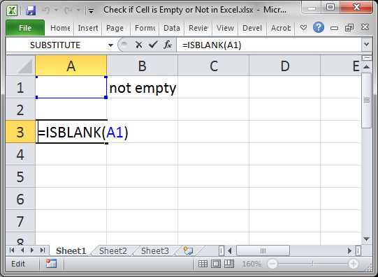
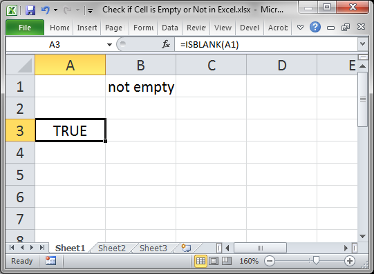
This will return TRUE if the cell is empty or FALSE if the cell is not empty.
Here, cell A1 is being checked, which is empty.
When the cell is not empty, it looks like this:
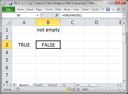
FALSE is output because cell B1 is not empty.
Reverse the True/False Output
Some formulas need to have TRUE or FALSE reversed in order to work correctly; to do this, use the NOT() function.
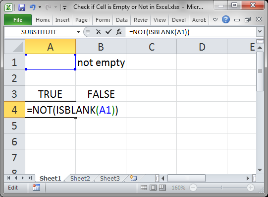
Result:
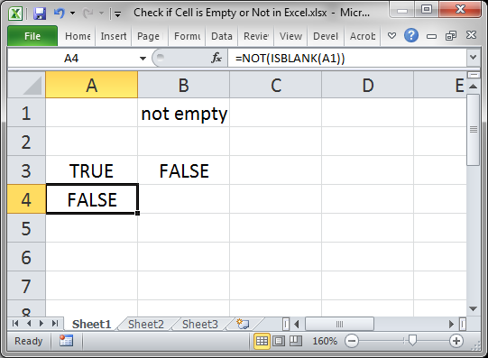
Whereas ISBLANK() output a TRUE for cell A1, the NOT() function reversed that and changed it to FALSE.
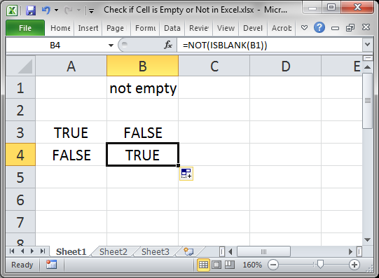
The same works for changing FALSE to TRUE.
Check if a Cell is Empty or Not — Method 2
You can also use an IF statement to check if a cell is empty.
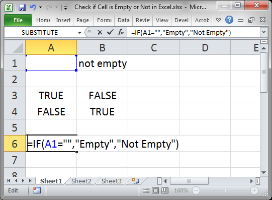
=IF(A1="","Empty","Not Empty")
Result:
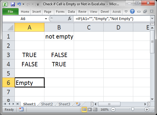
The function checks if this part is true: A1=»» which checks if A1 is equal to nothing.
When there is something in the cell, it works like this:
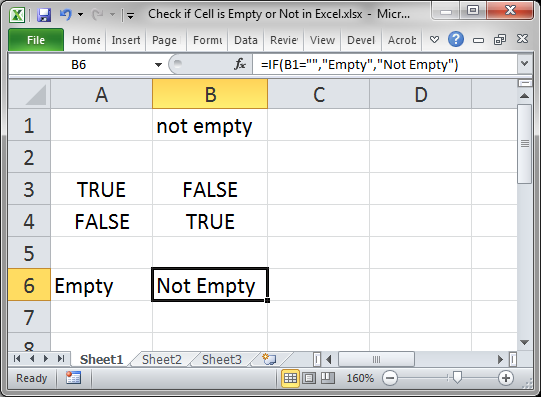
Cell B1 is not empty so we get a Not Empty result.
In this example I set the IF statement to output «Empty» or «Not Empty» but you can change it to whatever you like.
Reverse the Check
The example above checked if the cell was empty, but you can also check if the cell is not empty.
There are a few different ways to do this, but I will show you a simple and easy method here.
=IF(A1<>"","Not Empty","Empty")
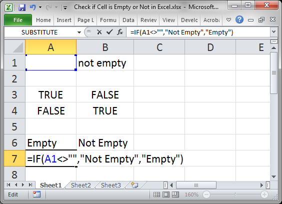
Notice the check this time is A1<>»» and that says «is cell A1 not equal to nothing.» It sounds confusing but just remember that <> is basically the reverse of =.
I also had to switch the «Empty» and «Not Empty» in order to get the correct result since we are now checking if the cell is not empty.
Result:
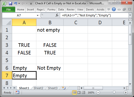
As you can see, it outputs the same result as the previous example, just like it should.
Using <> instead of = merely reverses it, making a TRUE become a FALSE and a FALSE become a TRUE, which is why «Empty» and «Not Empty» had to be reversed in order to still output the correct result.
Notes
It may seem useless to return TRUE or FALSE like in the first method, but remember that many functions in Excel, including IF(), AND(), and OR() all rely on results that are either TRUE or FALSE.
Checking for blanks and returning TRUE or FALSE is a simple concept but it can get a bit confusing in Excel, especially when you have complex formulas that rely on the result of the formulas in this tutorial. Save this tutorial and work with the attached sample file and you will have it down in no time.
Make sure to download the attached sample file to work with these examples in Excel.
Similar Content on TeachExcel
Excel VBA Check if a Cell is in a Range
Tutorial: VBA that checks if a cell is in a range, named range, or any kind of range, in Excel.
Sec…
Make Complex Formulas for Conditional Formatting in Excel
Tutorial: How to make complex formulas for conditional formatting rules in Excel. This will serve as…
Sort Data Alphabetically or Numerically in Excel 2007 and Later
Tutorial: This Excel tip shows you how to Sort Data Alphabetically and Numerically in Excel 2007. T…
Filter Data to Display the Results that Begin With Specified Text or Words in Excel — AutoFilter
Macro: This Excel macro automatically filters a set of data based on the words or text that are c…
Odd or Even Row Formulas in Excel
Tutorial: Formulas to determine if the current cell is odd or even; this allows you to perform speci…
Formula to Count Occurrences of a Word in a Cell or Range in Excel
Tutorial: Formula to count how many times a word appears in a single cell or an entire range in Exce…
Subscribe for Weekly Tutorials
BONUS: subscribe now to download our Top Tutorials Ebook!
In this tutorial, I explain three ways to display zeros as blanks. Download the featured file here.
Method One: Use the IF Function
Using the IF function we can return an empty text string in place of a zero result. In the example below the current stock level is calculated by subtracting the Sold value from the Stock Level value.

5 FREE EXCEL TEMPLATES
Plus Get 30% off any Purchase in the Simple Sheets Catalogue!
Using an IF function we can use a logical test that evaluates whether the current stock level equals zero. Watch this part of the video here.
=IF(C3-D3=0,””,C3-D3)
The value if true result is an empty text string “”
=IF(C3-D3=0,“”,C3-D3)
Method Two: Use Custom Formatting
The second method uses custom formatting to display zeros as blanks. Watch this part of the video here. To apply this custom formatting:
- Select the cells that you want to apply the formatting to
- Use the keyboard shortcut CTRL 1 to open the Format Cells dialog box
- Click on the Number tab in the Format Cells dialog box, if it is not already selected
- Select Custom in the Category list
- In the Type box type the following: 0;-0;;@ To get an explanation of this syntax, please watch the video beginning here.
Method Three: Worksheet Option
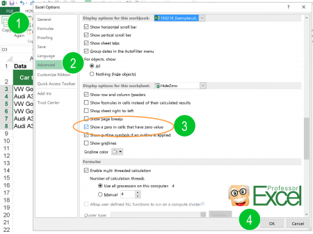
This method will hide zeros across the whole worksheet. Watch this part of the video here. To use this method:
- Select the Ribbon’s File tab
- Select Options
- In the Excel Options dialog, select Advanced down the left-side
- Scroll down to the section named Display options for this worksheet
- In the drop-down next to the section name, select your worksheet
- Untick the option Show a zero in cells that have zero value
- Click on OK.
If the return cell in an Excel formula is empty, Excel by default returns 0 instead. For example cell A1 is blank and linked to by another cell. But what if you want to show the exact return value – for empty cells as well as 0 as return values? This article introduces three different options for dealing with empty return values.
Option 1: Don’t display zero values
Probably the easiest option is to just not display 0 values. You could differentiate if you want to hide all zeroes from the entire worksheet or just from selected cells.
There are three methods of hiding zero values.
- Hide zero values with conditional formatting rules.
- Blind out zeros with a custom number format.
- Hide zero values within the worksheet settings.
For details about all three methods of just hiding zeroes, please refer to this article.

One small advice on my own account: My Excel add-in “Professor Excel Tools” has a built-in Layout Manager. With this, you can apply this formatting easily to a complete Excel workbook.
Give it a try? Click here and the download starts right away.
Option 2: Change zeroes to blank cells
Unlike the first option, the second option changes the output value. No matter if the return value is 0 (zero) or originally a blank cell, the output of the formula is an empty cell. You can achieve this using the IF formula.

Say, your lookup formula looks like this: =VLOOKUP(A3,C:D,2,FALSE) (hereafter referred to by “original formula”). You want to prevent getting a zero even if the return value―found by the VLOOKUP formula in column D―is an empty value. This can be achieved using the IF formula.
The structure of such IF formula is shown in the image above (if you need assistance with the IF formula, please refer to this article). The original formula is wrapped within the IF formula. The first argument compares if the original formula returns 0. If yes―and that’s the task of the second argument―the formula returns nothing through the double quotation marks. If the orgininal formula within the first argument doesn’t return zero, the last argument returns the real value. This is achieved by the original formula again.
The complete formula looks like this.
=IF(VLOOKUP(A3,C:D,2,FALSE)=0,"",VLOOKUP(A3,C:D,2,FALSE))
Do you want to boost your productivity in Excel?
Get the Professor Excel ribbon!

Add more than 120 great features to Excel!
Option 3: Show zeroes but don’t show blank or empty return values

The previous option two didn’t differentiate between 0 and empty cells in the return cell. If you only want to show empty cells if the return cell found by your lookup formula is empty (and not if the return value really is 0) then you have to slightly alter the formula from option 2 before.
Like before, the IF formula is wrapped around the original formula. But instead of testing if the return value is 0, it tests within the first argument if the return value is blank. This is done by the double quotation marks. The rest of the formula is the as before: With the second argument you define that—if the value from the original formula is blank—the return value is empty too. If not, the last argument defines that you return the desired non-blank value.
The formula in your example from option 2 looks like this.
=IF(VLOOKUP(A3,C:D,2,FALSE)="","",VLOOKUP(A3,C:D,2,FALSE))
Option 4: Use Professor Excel Tools to insert the IF functions very quickly
To save some time, we have included a feature for showing blank cells (instead of zeros) in our Excel add-in Professor Excel Tools.
It’s very simple:
- Select the cells that are supposed to return blanks (instead of zeros).
- Click on the arrow under the “Return Blanks” button on the Professor Excel ribbon and then on either
- Return blanks for zeros and blanks or
- Return zeros for zeros and blanks for blanks.
Professor Excel then inserts the IF function as shown in options 2 and 3 above.

This function is included in our Excel Add-In ‘Professor Excel Tools’
(No sign-up, download starts directly)
Option 5: One elegant solution for not returning zero values…

… was written in the comments. Thanks, Dom! Great to get such awesome feedback from you!
It’s actually quite straight forward: Add two quotation marks in front or after the function and concatenate it with the “&”-character. So, in this case the VLOOKUP function from above would look like this:
=""&VLOOKUP(A3,C:D,2,FALSE)
But: There is a downside. This method forces the cell to a text / string value. This might cause problems in further calculations if a zero is returned. Let me give you an example:
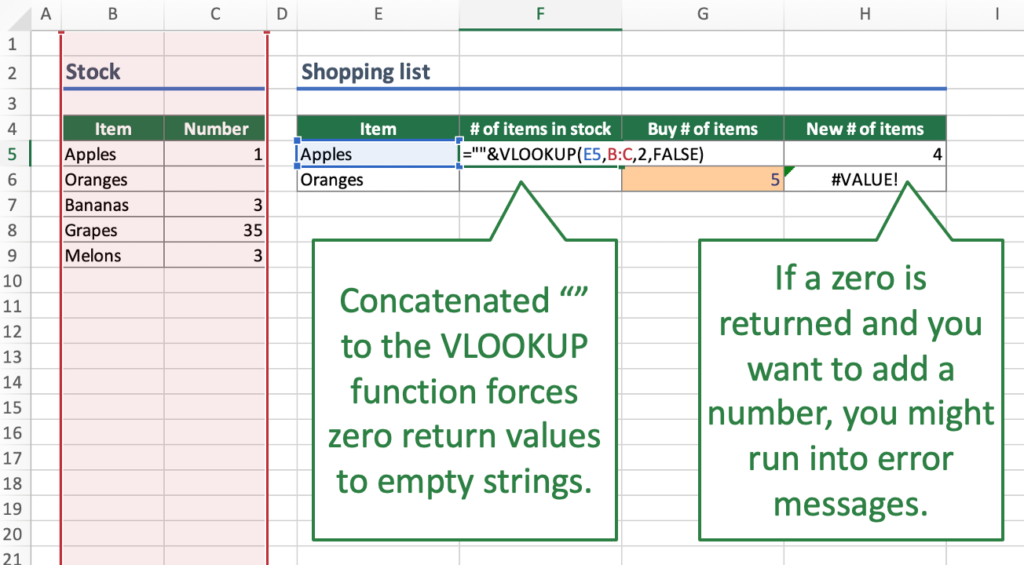
Careful: Return value is interpretated as text.Your VLOOKUP function above is concatenated to an empty string “”. If your return value is 0, the cell will be shown as an empty string. Further calculations might be difficult: For example, if you want to add a number to the return value. Referring directly to the cell, for example =F6+G6 leads to the #VALUE error message as shown above. However, using the SUM function =SUM(F6,G6) still works.
Bottom line: This is an elegant approach, but please test it well if it suits to your Excel model.
Image by Pexels from Pixabay
If Blank | If Not Blank | Highlight Blank Cells
Use the IF function and an empty string in Excel to check if a cell is blank. Use IF and ISBLANK to produce the exact same result.
If Blank
Remember, the IF function in Excel checks whether a condition is met, and returns one value if true and another value if false.
1. The IF function below returns Yes if the input value is equal to an empty string (two double quotes with nothing in between), else it returns No.

Note: if the input cell contains a space, it looks blank. However, if this is the case, the input value is not equal to an empty string and the IF function above will return No.
2. Use IF and ISBLANK to produce the exact same result.

Note: the ISBLANK function returns TRUE if a cell is empty and FALSE if not. If the input cell contains a space or a formula that returns an empty string, it looks blank. However, if this is the case, the input cell is not empty and the formula above will return No.
If Not Blank
In Excel, <> means not equal to.
1. The IF function below multiplies the input value by 2 if the input value is not equal to an empty string (two double quotes with nothing in between), else it returns an empty string.

2. Use IF, NOT and ISBLANK to produce the exact same result.

Highlight Blank Cells
You can use conditional formatting in Excel to highlight cells that are blank.
1. For example, select the range A1:H8.

2. On the Home tab, in the Styles group, click Conditional Formatting.

3. Click Highlight Cells Rules, More Rules.

4. Select Blanks from the drop-down list, select a formatting style and click OK.

Result.

Note: visit our page about conditional formatting to learn much more about this cool Excel feature.
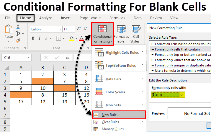
Table of Contents
- Conditional Formatting for Blank Cells
- How to Apply Conditional Formatting for Blank Cells?
Excel Conditional Formatting for Blank Cells
Conditional Formatting for Blank Cells is the function in excel that is used for creating inbuilt or customized formatting. From this, we can highlight the duplicate, color the cell as per different value ranges, etc. It also has a way to highlight blank cells.
How to Apply Conditional Formatting for Blank Cells?
To Apply Conditional Formatting for Blank Cells is very simple and easy. Let’s understand how to apply in excel.
You can download this Conditional Formatting For Blank Cells Excel Template here – Conditional Formatting For Blank Cells Excel Template
Example #1
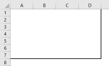
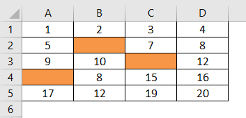
We will be covering the small portion of Conditional Formatting, which Highlights the Blank Cells. For this, consider a blank sheet. This is the best way to see and apply conditional formatting for a blank sheet or some of the cells of a blank sheet. If we apply the conditional formatting to complete a blank sheet or some cells of it, we will see how the cell gets highlighted. For this, we have selected a small portion of the sheet covered with a thick border, as shown below.
- We will apply the conditional formatting in a defined region only. For that, go to the Home menu and select Conditional Formatting under the Styles section, as shown below.
- Once we do that, we will get the drop-down list of Conditional Formatting. From that list, select New Rule.
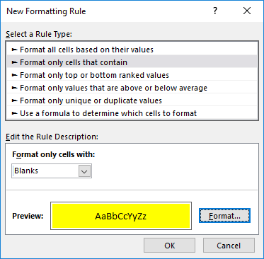
- A window of the New Formatting Rule will open up. There we have a different rule to apply conditional formatting. But for Blank cell, select the second option, which is Format only cells that contain.
- And below, in Edit the Rule Description box, we have different criteria to define. Here, from the very first box of drop-down, select Blanks as cell value.
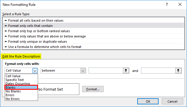
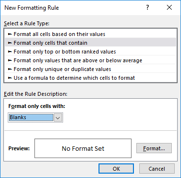
- Once we select the Blanks as cell value, all rest of the drop-down boxes will be eliminated from the condition. And we will get conditions related to Blank cells.
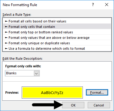
- Now for further, Click on the Format option from the same window as highlighted in the below screenshot.
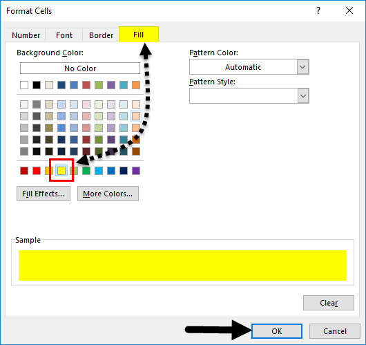
- The Format option will take us to the customize windows where we can change the text fonts, shape, or define or change the border or fill. For highlighting blank cells, go to the Fill tab and select any desired color as per requirement. We can also change the pattern as well. Once done, click on Ok, as shown below.
- After clicking on Ok, it will take us again back to the previous window, where we will get the preview of the selected color and condition as shown below.
- If the selected condition suits and matches the requirement, click Ok or select go back to Format to update the conditions. Here we got to apply conditions and rule as per our need. Now click on Ok.
- After clicking on Ok, we will get all the blank cells highlighted with Yellow color, as shown below.
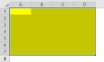
- Now to test, whether the condition which we have selected is applied properly or not, go to any of those cells and type anything to see if the cell color changes to No Fill or White background. As we can see, the cells with any value are now changed to a No Fill cell, as shown below.
Example #2
There is another way to apply conditional formatting to blank cells. And this method is quite easy to apply. For this, we have another set of data, as shown below.
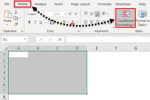
Now for applying Conditional Formatting, first select the data and follow the same path as shown in example-1.
- Go to the Home menu, under the Styles section, select Conditional Formatting.
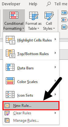
- Once we do that, we will get the drop-down list of all the available options under it. Now select the New Rule from the list.

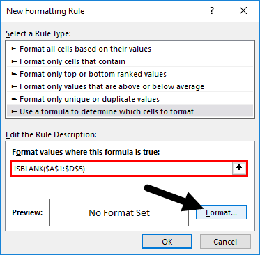
- Once we do that, we will get the New Formatting Rule box. There we have a different rule to apply conditional formatting. But here, we have to select the last option: “Use a formula to determine which cells to format”.
- Now in the Edit the Rule Description box, write the syntax of a function ISBLANK and select the complete range of data and after that, click on the Format tab, as shown below.
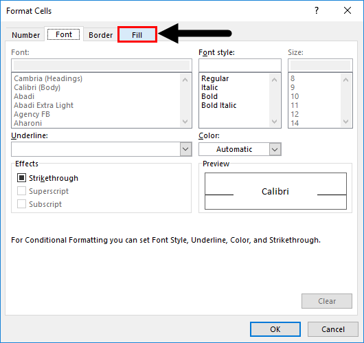
- Now a Format Cells window will open. Go to Fill tab.
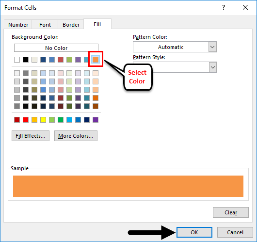
- And select the color of your choice to highlight the blank cells. Here we have selected the color as shown below. Once done. Click on OK to apply.
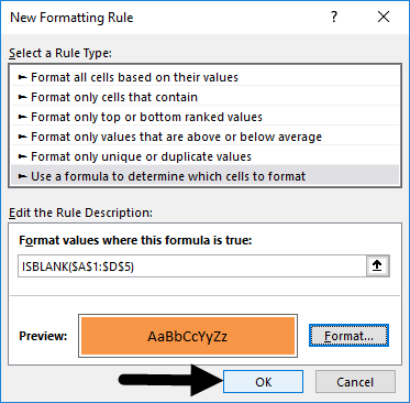
- After clicking on Ok, it will again take us back to the same previous window, where we will get the preview of the selected color and condition. Now click on Ok to apply.
- To test the applied condition, delete any of the cell data and see the result. We have deleted some cells data for testing, and the color of those cells change from No Fill to Red Peach. Which shows our selected and applied conditions are working properly.
Pros
- It is very quick and easy to apply.
- We can select any range and type of data to highlight blank cells.
- This is quite useful when we are working on data validation work. By this, we can highlight the cell and attributes which are left blank.
Cons
- Applying conditional formatting to large data set such as complete sheet may make excel work slow while filtering.
Things to Remember
- The selection of proper rules and formatting is very important. Once we select, it will always check and look for the preview before applying the changes.
- Always use limited data to deal with and apply bigger conditional formatting to avoid excel getting freeze.
Recommended Articles
This has been a guide to Conditional Formatting for Blank Cells. Here we discuss how to apply Conditional formatting for blank cells along with practical examples and a downloadable excel template. You can also go through our other suggested articles –
- Excel Conditional Formatting in the Pivot Table
- Use of Conditional Formatting In MS Excel
- Formatting Text in Excel
- Excel Conditional Formatting for Dates