Excel format cell as string

The TEXT function lets you change the way a number appears by applying formatting to it with format codes. It’s useful in situations where you want to display numbers in a more readable format, or you want to combine numbers with text or symbols.

Note: The TEXT function will convert numbers to text, which may make it difficult to reference in later calculations. It’s best to keep your original value in one cell, then use the TEXT function in another cell. Then, if you need to build other formulas, always reference the original value and not the TEXT function result.

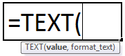
Syntax

TEXT(value, format_text)

The TEXT function syntax has the following arguments:

Argument Name	Description
value	A numeric value that you want to be converted into text.
format_text	A text string that defines the formatting that you want to be applied to the supplied value.

Overview

In its simplest form, the TEXT function says:

=TEXT(Value you want to format, «Format code you want to apply»)

Here are some popular examples, which you can copy directly into Excel to experiment with on your own. Notice the format codes within quotation marks.

Formula	Description
=TEXT(1234.567,«$#,##0.00»)	Currency with a thousands separator and 2 decimals, like $1,234.57. Note that Excel rounds the value to 2 decimal places.
=TEXT(TODAY(),«MM/DD/YY»)	Today’s date in MM/DD/YY format, like 03/14/12
=TEXT(TODAY(),«DDDD»)	Today’s day of the week, like Monday
=TEXT(NOW(),«H:MM AM/PM»)	Current time, like 1:29 PM
=TEXT(0.285,«0.0%»)	Percentage, like 28.5%
=TEXT(4.34 ,«# ?/?»)	Fraction, like 4 1/3
=TRIM(TEXT(0.34,«# ?/?»))	Fraction, like 1/3. Note this uses the TRIM function to remove the leading space with a decimal value.
=TEXT(12200000,«0.00E+00»)	Scientific notation, like 1.22E+07
=TEXT(1234567898,«[<=9999999]###-####;(###) ###-####»)	Special (Phone number), like (123) 456-7898
=TEXT(1234,«0000000»)	Add leading zeros (0), like 0001234
=TEXT(123456,«##0° 00′ 00»»)	Custom — Latitude/Longitude

Note: Although you can use the TEXT function to change formatting, it’s not the only way. You can change the format without a formula by pressing CTRL+1 (or +1 on the Mac), then pick the format you want from the Format Cells > Number dialog.

Download our examples

You can download an example workbook with all of the TEXT function examples you’ll find in this article, plus some extras. You can follow along, or create your own TEXT function format codes.

Download Excel TEXT function examples

Other format codes that are available

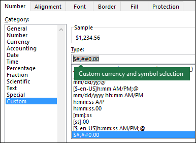
You can use the Format Cells dialog to find the other available format codes:

Press Ctrl+1 (+1 on the Mac) to bring up the Format Cells dialog.
Select the format you want from the Number tab.
Select the Custom option,
The format code you want is now shown in the Type box. In this case, select everything from the Type box except the semicolon (;) and @ symbol. In the example below, we selected and copied just mm/dd/yy.
Press Ctrl+C to copy the format code, then press Cancel to dismiss the Format Cells dialog.
Now, all you need to do is press Ctrl+V to paste the format code into your TEXT formula, like: =TEXT(B2,»mm/dd/yy«). Make sure that you paste the format code within quotes («format code»), otherwise Excel will throw an error message.

Format codes by category

Following are some examples of how you can apply different number formats to your values by using the Format Cells dialog, then use the Custom option to copy those format codes to your TEXT function.

Why does Excel delete my leading 0’s?

Excel is trained to look for numbers being entered in cells, not numbers that look like text, like part numbers or SKU’s. To retain leading zeros, format the input range as Text before you paste or enter values. Select the column, or range where you’ll be putting the values, then use CTRL+1 to bring up the Format > Cells dialog and on the Number tab select Text. Now Excel will keep your leading 0’s.

If you’ve already entered data and Excel has removed your leading 0’s, you can use the TEXT function to add them back. You can reference the top cell with the values and use =TEXT(value,»00000″), where the number of 0’s in the formula represents the total number of characters you want, then copy and paste to the rest of your range.

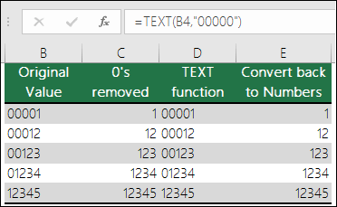
If for some reason you need to convert text values back to numbers you can multiply by 1, like =D4*1, or use the double-unary operator (—), like =—D4.

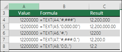
Excel separates thousands by commas if the format contains a comma (,) that is enclosed by number signs (#) or by zeros. For example, if the format string is «#,###», Excel displays the number 12200000 as 12,200,000.

A comma that follows a digit placeholder scales the number by 1,000. For example, if the format string is «#,###.0,», Excel displays the number 12200000 as 12,200.0.

Notes:

The thousands separator is dependent on your regional settings. In the US it’s a comma, but in other locales it might be a period (.).
The thousands separator is available for the number, currency and accounting formats.

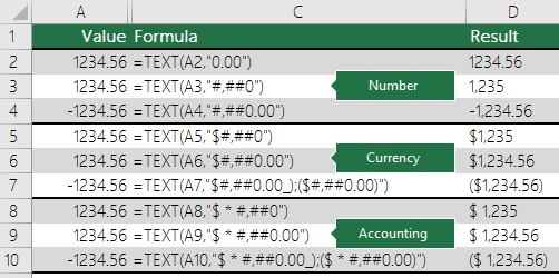
Following are examples of standard number (thousands separator and decimals only), currency and accounting formats. Currency format allows you to insert the currency symbol of your choice and aligns it next to your value, while accounting format will align the currency symbol to the left of the cell and the value to the right. Note the difference between the currency and accounting format codes below, where accounting uses an asterisk (*) to create separation between the symbol and the value.

To find the format code for a currency symbol, first press Ctrl+1 (or +1 on the Mac), select the format you want, then choose a symbol from the Symbol drop-down:

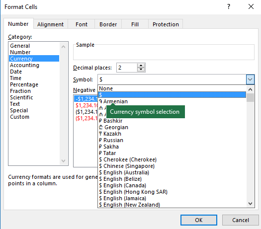
Then click Custom on the left from the Category section, and copy the format code, including the currency symbol.

Note: The TEXT function does not support color formatting, so if you copy a number format code from the Format Cells dialog that includes a color, like this: $#,##0.00_);[Red]($#,##0.00), the TEXT function will accept the format code, but it won’t display the color.

You can alter the way a date displays by using a mix of «M» for month, «D» for days, and «Y» for years.

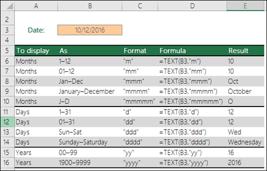
Format codes in the TEXT function aren’t case sensitive, so you can use either «M» or «m», «D» or «d», «Y» or «y».

You can alter the way time displays by using a mix of «H» for hours, «M» for minutes, or «S» for seconds, and «AM/PM» for a 12-hour clock.

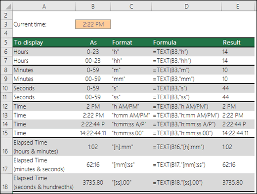
If you leave out the «AM/PM» or «A/P», then time will display based on a 24-hour clock.

Format codes in the TEXT function aren’t case sensitive, so you can use either «H» or «h», «M» or «m», «S» or «s», «AM/PM» or «am/pm».

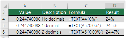
You can alter the way decimal values display with percentage (%) formats.

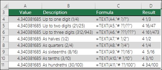
You can alter the way decimal values display with fraction (?/?) formats.

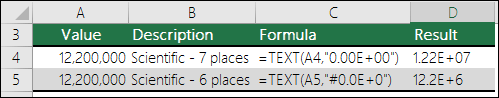
Scientific notation is a way of displaying numbers in terms of a decimal between 1 and 10, multiplied by a power of 10. It is often used to shorten the way that large numbers display.

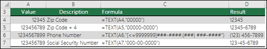
Excel provides 4 special formats:

Zip Code — «00000»
Zip Code + 4 — «00000-0000»
Phone Number — «[<=9999999]###-####;(###) ###-####»
Social Security Number — «000-00-0000»

Special formats will be different depending on locale, but if there aren’t any special formats for your locale, or if these don’t meet your needs then you can create your own through the Format Cells > Custom dialog.

Common scenario

The TEXT function is rarely used by itself, and is most often used in conjunction with something else. Let’s say you want to combine text and a number value, like “Report Printed on: 03/14/12”, or “Weekly Revenue: $66,348.72”. You could type that into Excel manually, but that defeats the purpose of having Excel do it for you. Unfortunately, when you combine text and formatted numbers, like dates, times, currency, etc., Excel doesn’t know how you want to display them, so it drops the number formatting. This is where the TEXT function is invaluable, because it allows you to force Excel to format the values the way you want by using a format code, like «MM/DD/YY» for date format.

In the following example, you’ll see what happens if you try to join text and a number without using the TEXT function. In this case, we’re using the ampersand (&) to concatenate a text string, a space (» «), and a value with =A2&» «&B2.

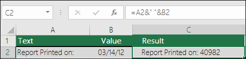
As you can see, Excel removed the formatting from the date in cell B2. In the next example, you’ll see how the TEXT function lets you apply the format you want.

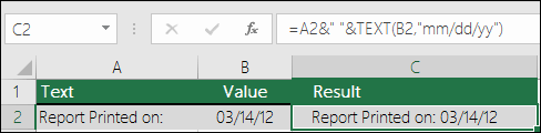
Our updated formula is:

Cell C2:=A2&» «&TEXT(B2,»mm/dd/yy») — Date format

Frequently Asked Questions

Yes, you can use the UPPER, LOWER and PROPER functions. For example, =UPPER(«hello») would return «HELLO».

Yes, but it takes a few steps. First, select the cell or cells where you want this to happen and use Ctrl+1 to bring up the Format > Cells dialog, then Alignment > Text control > check the Wrap Text option. Next, adjust your completed TEXT function to include the ASCII function CHAR(10) where you want the line break. You might need to adjust your column width depending on how the final result aligns.

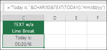
In this case, we used: =»Today is: «&CHAR(10)&TEXT(TODAY(),»mm/dd/yy»)

This is called Scientific Notation, and Excel will automatically convert numbers longer than 12 digits if a cell(s) is formatted as General, and 15 digits if a cell(s) is formatted as a Number. If you need to enter long numeric strings, but don’t want them converted, then format the cells in question as Text before you input or paste your values into Excel.

Description

The Microsoft Excel FORMAT function takes a string expression and returns it as a formatted string.

The FORMAT function is a built-in function in Excel that is categorized as a String/Text Function. It can be used as a VBA function (VBA) in Excel. As a VBA function, you can use this function in macro code that is entered through the Microsoft Visual Basic Editor.

Syntax

The syntax for the FORMAT function in Microsoft Excel is:

Format ( expression, [ format ] )

Parameters or Arguments

expression

The string value to format.

format

Optional. It is the format to apply to the expression. You can either define your own format or use one of the named formats that Excel has predefined such as:

Format	Explanation
General Number	Displays a number without thousand separators.
Currency	Displays thousand separators as well as two decimal places.
Fixed	Displays at least one digit to the left of the decimal place and two digits to the right of the decimal place.
Standard	Displays the thousand separators, at least one digit to the left of the decimal place, and two digits to the right of the decimal place.
Percent	Displays a percent value — that is, a number multiplied by 100 with a percent sign. Displays two digits to the right of the decimal place.
Scientific	Scientific notation.
Yes/No	Displays No if the number is 0. Displays Yes if the number is not 0.
True/False	Displays False if the number is 0. Displays True if the number is not 0.
On/Off	Displays Off if the number is 0. Displays On is the number is not 0.
General Date	Displays date based on your system settings
Long Date	Displays date based on your system’s long date setting
Medium Date	Displays date based on your system’s medium date setting
Short Date	Displays date based on your system’s short date setting
Long Time	Displays time based on your system’s long time setting
Medium Time	Displays time based on your system’s medium time setting
Short Time	Displays time based on your system’s short time setting

Returns

The FORMAT function returns a string value.

Applies To

Excel for Office 365, Excel 2019, Excel 2016, Excel 2013, Excel 2011 for Mac, Excel 2010, Excel 2007, Excel 2003, Excel XP, Excel 2000

Type of Function

VBA function (VBA)

Example (as VBA Function)

The FORMAT function can only be used in VBA code in Microsoft Excel.

Let’s look at some Excel FORMAT function examples and explore how to use the FORMAT function in Excel VBA code:

Format("210.6", "#,##0.00")
Result: '210.60'

Format("210.6", "Standard")
Result: '210.60'

Format("0.981", "Percent")
Result: '98.10%'

Format("1267.5", "Currency")
Result: '$1,267.50'

Format("Sep 3, 2003", "Short Date")
Result: '9/3/2003'

For example:

Dim LValue As String

LValue = Format("0.981", "Percent")

In this example, the variable called LValue would now contain the value of ‘98.10%’.

Источник

Excel is a great tool which can be used for data entry, as a database, and to analyze data and create dashboards and reports.

While most of the in-built features and default settings are meant to be useful and save time for the users, sometimes, you may want to change things a little.

Converting your numbers into text is one such scenario.

In this tutorial, I will show you some easy ways to quickly convert numbers to text in Excel.

Why Convert Numbers to Text in Excel?

When working with numbers in Excel, it’s best to keep these as numbers only. But in some cases, having a number could actually be a problem.

Lets look at a couple of scenarios where having numbers creates issues for the users.

Keeping Leading Zeros

For example, if you enter 001 in a cell in Excel, you will notice that Excel automatically removes the leading zeros (as it thinks these are unnecessary).

While this is not an issue in most cases (as you wouldn’t leading zeros), in case you do need these then one of the solutions is to convert these numbers to text.

This way, you get exactly what you enter.

One common scenario where you might need this is when you’re working with large numbers – such as SSN or employee ids that have leading zeros.

Entering Large Numeric Values

Do you know that you can only enter a numeric value that is 15 digits long in Excel? If you enter a 16 digit long number, it will change the 16th digit to 0.

So if you are working with SSN, account numbers, or any other type of large numbers, there is a possibility that your input data is automatically being changed by Excel.

And what’s even worse is that you don’t get any prompt or error. It just changes the digits to 0 after the 15th digit.

Again, this is something that is taken care of if you convert the number to text.

Changing Numbers to Dates

This one erk a lot of people (including myself).

Try entering 01-01 in Excel and it will automatically change it to date (01 January of the current year).

So if you enter anything that is a valid date format in Excel, it would be converted to a date.

A lot of people reach out to me for this as they want to enter scores in Excel in this format, but end up getting frustrated when they see dates instead.

Again, changing the format of the cell from number to text will help keep the scores as is.

Now, let’s go ahead and have a look at some of the methods you can use to convert numbers to text in Excel.

Convert Numbers to Text in Excel

In this section, I will cover four different ways you can use to convert numbers to text in Excel.

Not all these methods are the same and some would be more suitable than others depending on your situation.

So let’s dive in!

Adding an Apostrophe

If you manually entering data in Excel and you don’t want your numbers to change the format automatically, here is a simple trick:

Add an apostrophe (‘) before the number

So if you want to enter 001, enter ‘001 (where there is an apostrophe before the number).

And don’t worry, the apostrophe is not visible in the cell. You will only see the number.

Number converted to text by adding an apostrophe

When you add an apostrophe before a number, it will change it to text and also add a small green triangle at the top left part of the cell (as shown in th image). It’s Exel way to letting you know that the cell has a number that has been converted to text.

When you add an apostrophe before a number, it tells Excel to consider whatever follows as text.

A quick way to visually confirm whether the cells are formatted as text or not is to see whether the numbers align to the left out to the right. When numbers are formatted as text, they align to the right by default (as they alight to the left)

Adding an apostrophe changes cell alignment to left

Even if you add an apostrophe before a number in a cell in Excel, you can still use these as numbers in calculations

Similarly, if you want to enter 01-01, adding an apostrophe would make sure that it doesn’t get changed into a date.

Although this technique works in all cases, it is only useful if you’re manually entering a few numbers in Excel. If you enter a lot of data in a specific range of rows/columns, use the next method.

Converting Cell Format to Text

Another way to make sure that any numeric entry in Excel is considered a text value is by changing the format of the cell.

This way, you don’t have to worry about entering an apostrophe every time you manually enter the data.

You can go ahead entering the data just like you usually do, and Excel would make sure that your numbers are not changed.

Here is how to do this:

Select the range or rows/column where you would be entering the data
Click the Home tab

In the Number group, click on the format drop down

Select Text from the options that show up

The above steps would change the default formatting of the cells from General to Text.

Now, if you enter any number or any text string in these cells, it would automatically be considered as a text string.

This means that Excel would not automatically change the text you enter (such as truncating the leading zeros or converting entered numbers into dates)

In this example, while I changed the cell formatting first before entering the data, you can also do this with cells that already have data in them.

But remember that if you already had entered numbers that were changed by Excel (such as removing leading zeros or changing text to dates), that won’t come back. You will have to make that data entry again.

Also, keep in mind that cell formatting can change in case you copy and paste some data to these cells. With regular copy-paste, it also copied the formatting from the copied cells. So it’s best to copy and paste values only.

Using the TEXT Function

Excel has an in-built TEXT function that is meant to convert a numeric value to a text value (where you have to specify the format of the text in which you want to get the final result).

This method is useful when you already have a set of numbers and you want to show them in a more readable format or if you want to add some text as suffix or prefix to these numbers.

Suppose you have a set of numbers as shown below, and you want to show all these numbers as five-digit values (which means to add leading zeros to numbers that are less than 5 digits).

Dataset with numbers of different digits

While Excel removes any leading zeros in numbers, you can use the below formula to get this:

=TEXT(A2,"00000")

In the above formula, I have used “00000” as the second argument, which tells the formula the format of the output I desire. In this example, 00000 would mean that I need all the numbers to be at least five-digit long.

You can do a lot more with the TEXT function – such as add currency symbol, add prefix or suffix to the numbers, or change the format to have comma or decimals.

Using this method can be useful when you already have the data in Excel and you want to format it in a specific way.

This can also be helpful in saving time when doing manual data entry, where you can quickly enter the data and then use the TEXT function to get it in the desired format.

Using Text to Columns

Another quick way to convert numbers to text in Excel is by using the Text to Columns wizard.

While the purpose of Text to Columns is to split the data into multiple columns, it has a setting that also allows us to quickly select a range of cells and convert all the numbers into text with a few clicks.

Suppose you have a data set is shown below, and you want to convert all the numbers in columns A into text.

Below are the steps to do this:

Select the numbers in Column A
Click the Data tab

Click on the Text to Columns icon in the ribbon. This will open the text to columns wizard this will open the text to column wizard

In Step 1 of 3, click the Next button
In Step 2 of 3, click the Next button
In Step 3 of 3, under the ‘Column data format’ options, select Text

Select Text option in the Text to Columns Wizard

Click on Finish

The above steps would instantly convert all these numbers in Column A into text. You notice that the numbers would now be aligned to the right (indicating that the cell content is text).

There would also be a small green triangle at the top left part of the cell, which is a way Excel informs you that there are numbers that are stored as text.

So these are four easy ways that you can use to quickly convert numbers to text in Excel.

In case you only want this for a few cells where you would be manually entering the data, I suggest you use the apostrophe method. If you need to do data entry for more than a few cells, you can try changing the format of the cells from General to Text.

And in case you already have the numbers in Excel and you want to convert them to text, you can use the TEXT formula method or the Text to Columns method I covered in this tutorial.

I hope you found this tutorial useful.

Other Excel tutorials you may also like:

Convert Text to Numbers in Excel
How to Convert Serial Numbers to Dates in Excel
Convert Date to Text in Excel – Explained with Examples
How to Convert Formulas to Values in Excel
Convert Time to Decimal Number in Excel
How to Convert Inches to MM, CM, or Feet in Excel?
Convert Scientific Notation to Number or Text in Excel
Separate Text and Numbers in Excel

Источник

The TEXT excel function converts a number to a text string based on the format specified by the user. This format is supplied as an argument to the TEXT function. Since the resulting outputs are text representations of numbers, they cannot be used as is in formulas. Therefore, it is recommended to retain the original numbers and create a separate row or column for the converted numbers.

For example, the formula “=TEXT(“10/2/2022″,”mmmm dd, yyyy”)” returns February 10, 2022. Exclude the beginning and ending double quotation marks while entering this formula in Excel.

The purpose of using the TEXT function in Excel is to display a number in the desired format. Since this function also helps combine numbers with other text strings, it tends to make the output more legible. The TEXT function is particularly used when the number formats of different datasets need to be made identical.

Estimated reading time: 21 minutes

What is Text Function in Excel?
- Syntax of the TEXT Function of Excel
- How to Use the TEXT Function in Excel?
  - Example #1–Prefix the Text Strings to the Newly Formatted Date Values
  - Example #2–Join the Newly Formatted Time and Date Values
  - Example #3–Extract a Mobile Number from its Scientific Notation
  - Example #4–Prefix a Text String to the Initially Formatted Monetary Value
- Date Formats of Excel
- Frequently Asked Questions
- TEXT Function in Excel Video
- Recommended Articles

Syntax of the TEXT Function of Excel

The syntax of the TEXT function of Excel is shown in the following image:

The TEXT function of Excel accepts the following arguments:

Value: This is the number to be converted to a text string. Apart from a number, a date, time or cell reference can also be supplied to the TEXT excel function. The cell reference can contain either a number or an output of another function which can be a number or date.
Format_text: This is the format to be applied to the “value” argument. It is also called the format code. It is entered within double quotation marks in the TEXT formula of Excel. For instance, “0.00,” “dd/mm/yyyy,” “hh:mm:ss,” and so on are format codes.

Both the stated arguments are mandatory.

Note 1: The format code “0.00” displays a number with two decimal places. In the format code “dd/mm/yyyy,” “dd,” “mm,” and “yyyy” are the notations for days (in two digits), months (in two digits), and years (in four digits) respectively.

Likewise, “hh,” “mm,” and “ss” are the notations for hours (in two digits), minutes (in two digits), and seconds (in two digits) respectively.

For the meaning of the different date formats, refer to the heading “date formats of Excel” given after example #4 of this article.

Note 2: The TEXT function is categorized as a Text/String function of Excel. The TEXT function is available in all versions of Excel.

How to Use the TEXT Function in Excel?

Let us consider some examples to understand the working of the TEXT function in Excel.

Example #1–Prefix the Text Strings to the Newly Formatted Date Values

The following table shows the names of five children along with the dates they were born on. The dates are currently in the format m/d/yyyy. Consider the two columns and six rows of the table as columns A and B and rows 1 to 6 of Excel.

We want to perform the following tasks:

Join the name and date of birth of row 2 by using the ampersand operator. There should not be any space between the joined values.
Convert each date to the format “dd mmm, yyyy.” Prefix the child’s name and the string “was born on” to each date.
Show the output when the date of row 2 is in the format “d mmm, yyyy.” Let the prefixes of the preceding point stay as it is.
Show the date formats “dd mmm, yyyy” (in cell C2) and “d mmm, yyyy” (in cell C6) in a single column.

Explain the outputs obtained in the second and fourth bullet points. Use the TEXT function of Excel.

Name of Kid	Date of Birth
John	12/8/2015
Patricia	1/12/2014
Ram	3/11/2016
Anita	11/11/2017
Davis	5/6/2014

The steps to perform the given tasks by using the TEXT function of Excel are listed as follows:

Step 1: Enter the following formula in cell C2. Exclude the beginning and ending double quotation marks while entering the given formula.

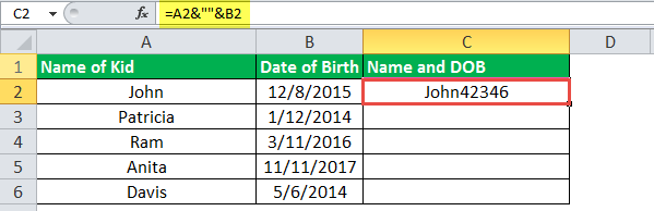
“=A2&“”&B2”

This formula (shown in the image of step 2) joins the values of cells A2 and B2 without any spaces in-between.

Note: The ampersand operator (&) helps join the values of two or more cells. It is called the concatenation operator and is used as an alternative to the CONCATENATE function of Excel. There is no limit on the number of cell values that the ampersand can join.

Step 2: Press the “Enter” key. The output appears in cell C2, as shown in the following image.

Notice that Excel has joined the values of cells A2 and B2 without any spaces in-between. However, the output is not in a readable format. The reason is that the date (12/8/2015) has been converted to a sequential number. The number 42346 represents the date December 8, 2015.

Note: A date is stored in Excel as a sequential or a serial number. This is because a serial number makes it easy to perform calculations. To view the serial number of a date, refer to the “note” preceding step 3 of example #2.

Step 3: To apply the format “dd mmm, yyyy” and insert the stated prefixes, enter the following formula in cell C2.

“=A2&” was born on “&TEXT(B2,”dd mmm, yyyy”)”

Press the “Enter” key. Then, drag the formula of cell C2 till cell C6 by using the fill handle. The outputs are displayed in the following image.

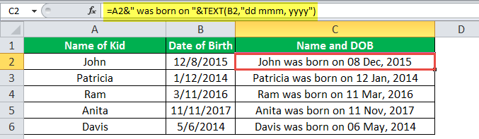
Explanation of the outputs: In column C of the preceding image, the child’s name (in column A) and the text string (was born on) have been prefixed to each date of column B. Since the date is in a suitable format, the output is readable now.

The joined values (outputs) of column C are in the form of statements that are easier to understand than the single values of columns A and B.

Notice that, to insert spaces as the separators in the output, we have inserted spaces at the relevant places in the formula of step 1. Moreover, a comma has also been inserted after the notation of months (mmm). This comma can be seen in each date of the output (in column C).

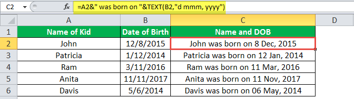
Step 4: To see the output when the date format is “d mmm, yyyy” and the prefixes are in place, enter the following formula in cell C2.

=A2&” was born on “&TEXT(B2,”d mmm, yyyy”)

Press the “Enter” key. The output appears in cell C2, as shown in the following image.

Notice that the leading zero before the date 8 Dec, 2015 (in cell C2) has disappeared. This zero was there in cell C2 of the preceding image. It has disappeared because, in the current format code, the number of days is represented by a single “d.”

A single “d” omits the leading zeros when the number of days is in a single digit.

Step 5: The outputs obtained after applying different date formats in the same column (column C) are shown in the following image.

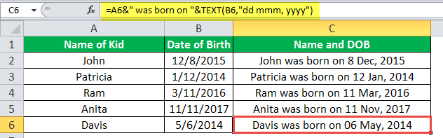
Explanation of the outputs: Notice that in the preceding image, the date of cell C2 is in the format “d mmm, yyyy” while that of cell C6 is in the format “dd mmm, yyyy.” The only difference between these two date formats is in the number of days. The leading zero is absent in cell C2 and present in cell C6.

Hence, with the TEXT function of Excel, one can have different date formats in different cells of the same column. Remember that a format code changes only the appearance of a value; it does not change the value itself. One can create a format code depending on the requirement.

Example #2–Join the Newly Formatted Time and Date Values

The following table shows the times and dates in two separate columns. Consider these columns as columns A and B of Excel. We want to perform the following tasks:

Join (concatenate) each time value with the respective date. Use the ampersand operator (&) and ensure that there is no space between the two values.
Show how to copy the formats “h:mm:ss am/pm” and “m/d/yyyy” from the “format cells” window. Convert each time to the former and date to the latter format.
Join the converted time and date values with the ampersand operator (&). Ensure that there is a space between the two values.
Show the output when the date format is not enclosed within double quotation marks.

Explain the outputs obtained in the first and third bullet points. Use the TEXT function of Excel for the given tasks.

Time	Date
7:00:00 AM	6/19/2018
7:15:00 AM	6/19/2018
7:30:00 AM	6/19/2018
7:45:00 AM	6/19/2018
8:00:00 AM	6/19/2018
8:15:00 AM	6/19/2018
8:30:00 AM	6/19/2018
8:45:00 AM	6/19/2018

The steps to perform the given tasks by using the TEXT function of Excel are listed as follows:

Step 1: Enter the following formula (without the beginning and ending double quotation marks) in cell C2.

“=A2&“”&B2”

This formula is shown in the image of step 2. It joins the values of cells A2 and B2 without a space in-between.

Step 2: Press the “Enter” key. Then, drag the formula of cell C2 till cell C9 by using the fill handle. The fill handle is displayed at the bottom-right side of cell C2.

The outputs are shown in the following image.

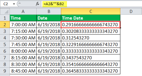
Explanation of the outputs: In column C, the number 43270 (at the end) is the same throughout the range C2:C9. This is the serial number for the date June 19, 2018. The entire decimal number preceding this serial number is the time. So, the decimal number 0.2916667 (in cell C2) represents the time 7:00:00 am.

The outputs obtained in column C of the preceding image are not readable. The reason is that Excel has converted the times (of column A) to decimal numbers and dates (of column B) to sequential numbers. Moreover, joining the decimals with sequential numbers has made the outputs more complicated.

To be able to read the output, it needs to be converted to the relevant format codes. This conversion is shown further in this example.

Note: Excel stores dates as sequential (or serial) numbers and times as decimal numbers. Excel considers a time value as a part of a day. To view the number representing the date, perform the following actions:

Select any cell of the range B2:B9.
Press the keys “Ctrl+1” together. The “format cellsFormatting cells is an important technique to master because it makes any data presentable, crisp, and in the user’s preferred format. The formatting of the cell depends upon the nature of the data present.read more” window opens.
Select “general” under “category” in the “number” tab.

The serial number can be seen under “sample.” Click “cancel” to close the “format cells” window or “Ok” to change the date to a serial number.

Likewise, the decimal number representing the time can also be seen by selecting any cell of the range A2:A9 and following actions “b” and “c” listed above.

Step 3: To convert the time and date values to a readable format, let us first copy the format codes from the “format cells” window. So, select cell C2 and press the keys “Ctrl+1” together.

The “format cells” window opens, as shown in the following image. From the “number” tab, select “custom” under “category. Excel provides a list of formats under “type.”

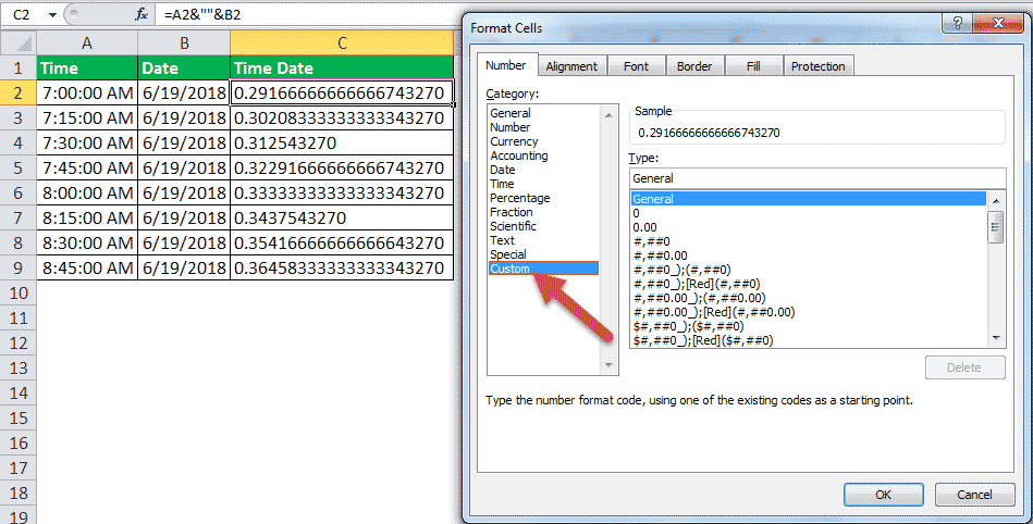
Step 4: Scroll down the list of formats given under “type.” Copy the format “h:mm:ss am/pm.” To copy, just select the format code and press the keys “Ctrl+C.”

The format code is shown in the following image. Once the format has been copied, close the “format cells” window.

Step 5: Copy the format code “m/d/yyyy” for converting the date values. This format code is also available under “type,” as shown in the following image.

Close the “format cells” window after copying the mentioned format code.

Step 6: To apply the new formats to the time and date values and join the resulting values, enter the following formula in cell C2.

“=TEXT(A2,”h:MM:SS AM/PM”)&” “&TEXT(B2,”m/d/yyyy”)”

This formula is shown in the image of step 7. If the format codes have been copied in the preceding steps, they can be pasted at the relevant places in the formula by pressing the shortcut “Ctrl+V.”

According to this formula, the time and date values of cells A2 and B2 are formatted as per the codes “h:MM:SS AM/PM” and “m/d/yyyy” respectively. The formatted (or converted) values are then joined with the ampersand operator.

Notice that in the formula, a space has also been entered within a pair of double quotation marks (like &“ ”&). This space will be inserted in the output at exactly that place where it has been entered in the formula.

Step 7: Press the “Enter” key after entering the TEXT formula. Drag the formula of cell C2 till cell C9.

The outputs are shown in the following image.

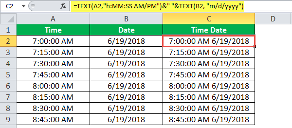
Explanation of the outputs: The time and date values of columns A and B have been converted to the relevant formats in column C. The time values display the hours (h) in a single digit, minutes (mm) in two digits, and seconds (ss) also in two digits. Since all the time values belong to the period before noon, they display “am” at the end.

Likewise, the dates display the months (m) in a single digit, days (d) in a single digit, and years (yyyy) in four digits.

Notice that there is a space between the two joined values in column C. Even though we copied the code “h:mm:ss am/pm” (in step 4) and pasted “h:MM:SS AM/PM” (in step 6), we obtained the correct outputs in column C (in step 7). This is because the format codes are not case-sensitive, implying that “mm” is treated the same as “MM.”

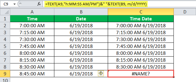
Step 8: To see what happens when the format code for date is entered without the double quotation marks, type the following formula in cell C9.

“=TEXT(A2,”h:MM:SS AM/PM”)&” “&TEXT(B2,m/d/YYYY)”

Press the “Enter” key. Excel returns the “#NAME?” error, as shown in the following image. Therefore, for the TEXT excel function to work, the format code should necessarily be enclosed within double quotation marks.

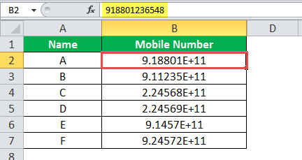
There are two images titled “image 1” and “image 2.” The following information is given:

Image 1 shows a number having eleven 9s in cell B2. When 1 is added to this number, its digits increase to 12. Excel displays the resulting 12-digit number (in cell B3) in a scientific notation.
Image 2 shows the names of some people (in column A) and their random mobile numbers in a scientific notation (in column B). The formula bar shows the mobile number of person A. Each mobile number consists of twelve digits, which includes a 2-digit country code at the beginning.

Note that a scientific notationIn Excel, scientific notation is a specific style of writing numbers in scientific and exponential forms. Scientific notation compactly helps display values, allowing us to compare and use the same in calculations.read more (or scientific format) often displays very large or very small numbers in a contracted form. We want to perform the following tasks:

Display the entire 12-digit mobile number without any spaces in-between.
Separate the country code from the rest of the number with the help of a hyphen.

Use the TEXT function of Excel for the given tasks.

Image 1

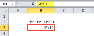
Image 2

The steps to perform the given tasks by using the TEXT function of Excel are listed as follows:

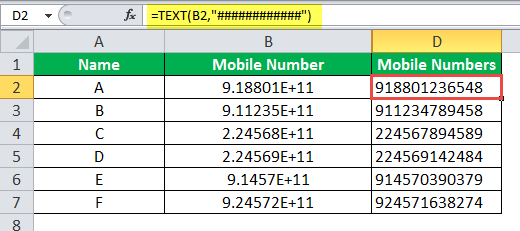
Step 1: Enter the following formula in cell D2.

“=TEXT(B2,”############”)”

This formula is shown in the formula bar of the succeeding image. Notice that there are 12 hashes in the formula, which represent the 12 digits of a mobile number.

Step 2: Press the “Enter” key. The output appears in cell D2. To obtain the outputs for the entire column D, drag the formula of cell D2 to cell D7. Use the fill handle of cell D2 (displayed at the bottom-right corner) for dragging.

The outputs of column D are shown in the succeeding image.

Note: The output is displayed (in column D) only when one enters a mobile number as an input (in column B) which is converted automatically (or manually) to a scientific format of Excel. In case, a scientific format is typed manually in column B; it cannot be converted to a mobile number of column D.

Step 3: To separate the country codes from the rest of the number by using a hyphen, enter the following formula in cell D2.

“=TEXT(B2,“##-##########”)”

Press the “Enter” key. Next, drag the formula of cell D2 till cell D7 with the help of the fill handle. The formula of cell D2 and the outputs are shown in the following image.

Notice that in the formula, the hyphen is placed exactly where it is required in the output. Since only the first two digits of each mobile number are to be separated, the hyphen is placed after two hashes of the formula.

Example #4–Prefix a Text String to the Initially Formatted Monetary Value

There are two images titled “image 1” and “image 2.” The following information is given:

Image 1 shows the gross profit, expenses, and net profit of an organization. All these numbers are in dollars.
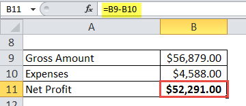
Image 2 shows how the net profit has been computed. To calculate the net profit, the expenses have been subtracted from the gross profit.

We want to perform the following tasks:

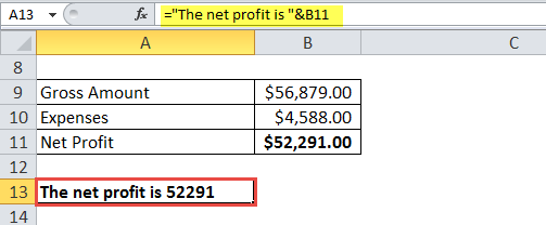
Show the output when the string “the net profit is” is prefixed to the amount of net profit. Use the ampersand operator for this purpose.
Prefix the string “the net profit is” to the amount of net profit by using the ampersand. Ensure that in the output, the amount of net profit displays the dollar sign ($) and the comma at the correct places (like $52,291). Use the TEXT function of Excel for this purpose.

Explain the output obtained at the end.

Image 1

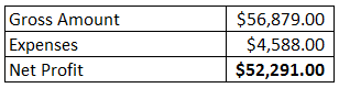
Image 2

The steps to perform the given tasks are listed as follows:

Step 1: Enter the following formula in cell A13.

“=”The net profit is “&B11”

Exclude the beginning and ending double quotation marks of the formula while entering it in Excel. This formula is shown in the image of step 2.

The given formula prefixes the string “the net profit is” to the value of cell B11. The ampersand helps join the stated string to the amount of net profit (in cell B11).

Step 2: Press the “Enter” key. The output appears in cell A13, as shown in the following image.

Notice that the dollar sign and the comma of the net profit amount (shown in cell B11) have been omitted in the output. Though the string “the net profit is” has been correctly prefixed. The spaces have also been inserted at the right places in cell A13.

Step 3: To retain the dollar sign and the comma of the amount, enter the following formula in cell A13.

“=”The net profit is ” &TEXT(B11,”$#,##0.00″)”

Press the “Enter” key. The formula and the output are shown in cell A13 of the following image.

Notice that by mistake, a space has been inserted before the ampersand in the formula. However, even then, the correct output has been obtained in cell A13.

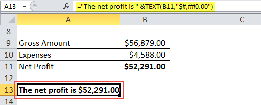
Explanation of the output: This time, the amount of net profit has been properly written (including the dollar sign and the comma) in cell A13. The reason is that the amount of net profit has been converted to the appropriate format in addition to being prefixed by a text string.

So, with the TEXT function of Excel, one can join a number with any string and, at the same time, retain the initial formatting of the number.

Date Formats of Excel

The different format codes for dates have been described as follows:

Frequently Asked Questions

1. Define the TEXT function in Excel with the help of an example.

The TEXT function in Excel helps convert a numerical value to a text string. The conversion is carried out according to the format specified by the user. Once converted, the numerical value becomes a text representation of a number.

The formula “=TEXT(“2/12/2021”,“dddd-mmmm-yyyy”)” converts the date 2/12/2021 to Thursday-December-2021. Ensure that the beginning and ending double quotation marks are excluded while entering this TEXT formula in Excel.

Note: For the working of the TEXT function of Excel, refer to the examples of this article.

2. Why is the TEXT function used in Excel?

The TEXT function is used in Excel for the following reasons:

• It helps convert a numerical value to a text string having a new format.
• It eases joining a numerical value with a text string.
• It helps retain the format of the existing numerical value after concatenation (joining).
• It makes the date or time values given in sequential or decimal numbers more readable and understandable for the users.
• It helps add the leading zeros to a number.
• It allows inserting specific characters (like +,-,(),<>,: etc.) in the output.

Note: The different characters that can be entered in the TEXT formula are the plus (+), minus (-), equal to (=), parentheses (), less than and greater than signs <>, colon (:), apostrophe (‘), curly braces {}, caret (^), forward slash (/), ampersand (&), space ( ), tilde (~), and an exclamation point (!).

The characters should be entered in the format code. These characters are displayed at exactly those places (in the output) where they have been entered in the format code.

3. How is the TEXT function used to add the leading zeros to a number in Excel?

The steps to add the leading zeros to a number are listed as follows:

a. Type “=TEXT” followed by the opening parenthesis.
b. Enter the number as the “value” argument.
c. Enter those many zeros in the format code as the number of digits required in the output.
d. Close the parenthesis and press the “Enter” key.

The leading zeros are added to the number entered in step “b.”

For instance, if the number 148 should appear as a 5-digit number, enter the formula “=TEXT(“148”,“00000”)” without the beginning and ending double quotation marks. It returns 00148.

TEXT Function in Excel Video

Where to install the macro: Module

Excel Macro to Format Cells as Text in Excel

Sub Format_Cell_Text()

Selection.NumberFormat = "@"

End Sub

Excel VBA Course — From Beginner to Expert

200+ Video Lessons
50+ Hours of Instruction
200+ Excel Guides

Become a master of VBA and Macros in Excel and learn how to automate all of your tasks in Excel with this online course. (No VBA experience required.)

View Course

Excel VBA Course — From Beginner to Expert

200+ Video Lessons

50+ Hours of Video

200+ Excel Guides

Become a master of VBA and Macros in Excel and learn how to automate all of your tasks in Excel with this online course. (No VBA experience required.)

View Course

Источник

Overview

Download our examples

Other format codes that are available

Format codes by category

Common scenario

Frequently Asked Questions

See Also

Description

Syntax

Parameters or Arguments

Returns

Applies To

Type of Function

Example (as VBA Function)

Why Convert Numbers to Text in Excel?

Keeping Leading Zeros

Entering Large Numeric Values

Changing Numbers to Dates

Convert Numbers to Text in Excel

Adding an Apostrophe

Converting Cell Format to Text

Using the TEXT Function

Using Text to Columns

Table of contents

Syntax of the TEXT Function of Excel

How to Use the TEXT Function in Excel?

Example #1–Prefix the Text Strings to the Newly Formatted Date Values

Example #2–Join the Newly Formatted Time and Date Values

Example #4–Prefix a Text String to the Initially Formatted Monetary Value

Date Formats of Excel

Frequently Asked Questions

TEXT Function in Excel Video

Recommended Articles

Where to install the macro: Module

Excel Macro to Format Cells as Text in Excel

Excel VBA Course — From Beginner to Expert

Excel VBA Course — From Beginner to Expert