Format numbers as percentages
Excel for Microsoft 365 Excel for Microsoft 365 for Mac Excel for the web Excel 2021 Excel 2021 for Mac Excel 2019 Excel 2019 for Mac Excel 2016 Excel 2016 for Mac Excel 2013 Excel 2010 Excel 2007 Excel for Mac 2011 More…Less
Learn how to display numbers as percentages in Excel and view examples of several basic techniques for calculating percentages in your worksheet.
In this article
-
How Excel handles percentages
-
Display numbers as percentages
-
Tips for displaying percentages
-
Examples of calculating percentages
-
Example 1: Increase or decrease a number by a percentage
-
Example 2: Calculate an amount based on a percentage
-
Example 3: Calculate the percentage based on two amounts
-
Example 4: Calculate an amount based another amount and a percentage
-
Example 5: Calculate the difference between two numbers and show it as a percentage
-
How Excel handles percentages
Although formatting numbers as percentages is straightforward, the results you get after you apply the format may vary, depending on whether the numbers already exist in your workbook.
-
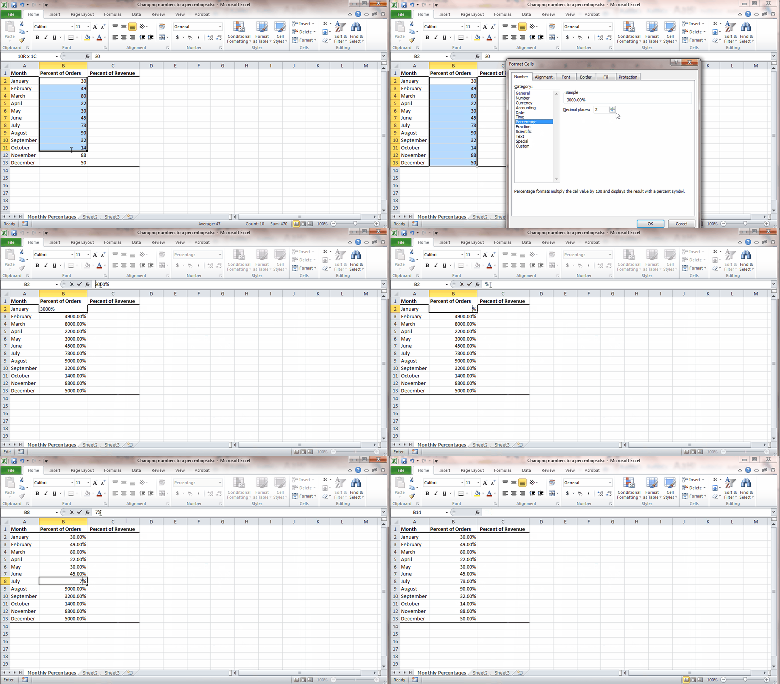
Formatting cells that already contain numbers If you apply the Percentage format to existing numbers in a workbook, Excel multiplies those numbers by 100 to convert them to percentages. For example, if a cell contains the number 10, Excel multiplies that number by 100, which means that you will see 1000.00% after you apply the Percentage format. This may not be what you expected. To accurately display percentages, before you format the numbers as a percentage, make sure that they have been calculated as percentages, and that they are displayed in decimal format. Percentages are calculated by using the equation amount / total = percentage. For example, if a cell contains the formula =10/100, the result of that calculation is 0.1. If you then format 0.1 as a percentage, the number will be correctly displayed as 10%. To learn more about calculating percentages, see Examples of calculating percentages.
-
Formatting empty cells If you apply the Percentage format to cells, and then type numbers into those cells, the behavior is different. Numbers equal to and larger than 1 are converted to percentages by default; and numbers smaller than 1 are multiplied by 100 to convert them to percentages. For example, typing 10 or 0.1 both result in 10.00%. (If you don’t want to display the two zeros after the decimal point, it’s easy to get rid of them, as explained in the following procedure.)
Top of Page
Display numbers as percentages
To quickly apply percentage formatting to selected cells, click Percent Style 
-
On the Home tab, in the Number group, click the icon next to Number to display the Format Cells dialog box.
-
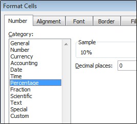
In the Format Cells dialog box, in the Category list, click Percentage.
-
In the Decimal places box, enter the number of decimal places that you want to display. For example, if you want to see 10% instead of 10.00%, enter 0 in the Decimal places box.
Top of Page
Tips for displaying percentages
-
To reset the number format of selected cells, click General in the Category list. Cells that are formatted with the General format have no specific number format.
-
If you want negative percentages to stand out—for example, you want them to appear in red—you can create a custom number format (Format Cells dialog box, Number tab, Custom category). The format should resemble the following: 0.00%;[Red]-0.00%. When applied to cells, this format displays positive percentages in the default text color and negative percentages in red. The portion that follows the semicolon represents the format that is applied to a negative value.
Similarly, you can display negative percentages in parentheses by creating a custom format that resembles this one: 0.00%_);(0.00%). For more information about how to create custom formats, see Create or delete a custom number format.
-
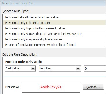
You can also use conditional formatting (Home tab, Styles group, Conditional Formatting) to customize the way negative percentages appear in your workbook. The conditional formatting rule you create should be similar to the one shown in the following example. This particular rule instructs Excel to apply a format (red text) to a cell if the cell value is less than zero. For more information about conditional formatting, see Add, change, find, or clear conditional formats.
Top of Page
Examples of calculating percentages
This section shows several simple techniques for calculating percentages.
Example 1: Increase or decrease a number by a percentage
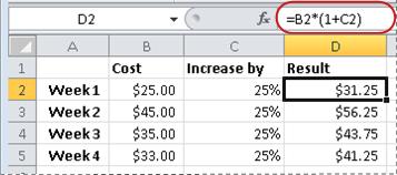
Scenario If you spend an average of $25 on food each week, and you want to cut your weekly food expenditures by 25%, how much can you spend? Or, if you want to increase your weekly food allowance of $25 by 25%, what is your new weekly allowance?
If B2 is the amount that you spend on food, and C2 is the percentage you want to decrease that amount by, you can enter =B2*(1-C2) in D2 to find the result:
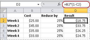
In this formula, 1 is used to represent 100%. Similarly, if you wanted to increase the amount by a certain percentage, you would enter =B2*(1+C2) in D2:
Top of Page
Example 2: Calculate an amount based on a percentage
Scenario If you purchase a computer for $800 and there is an 8.9% sales tax, how much do you have to pay for the sales tax? In this example, you want to find 8.9% of 800.
If B2 is the price and C2 is the sales tax, you can type the formula =B2*C2 in D2, as shown here:
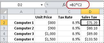
This formula multiplies 800 by 0.089 (the underlying percentage in decimal form) to find the sales tax to pay.
Top of Page
Example 3: Calculate the percentage based on two amounts
Scenario For example, if a student scored 42 points correctly out of 50 on a test, what is the percentage of correct answers?
In this scenario, if the number in B2 is points answered correctly and the number in C2 is the total points possible, you can type the formula =B2/C2 in D2 to find the grade.
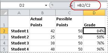
This formula divides 42 by 50 to find the percentage of correct answers. (In the example shown here, the grade is formatted as a percentage without any decimal places showing.)
Top of Page
Example 4: Calculate an amount based another amount and a percentage
Scenario For example, the sale price of a shirt is $15, which is 25% off the original price. What is the original price? In this example, you want to find 75% of which number equals 15.
If B2 is the sale price, and C2 is 0.75, which is 100% minus the 25% discount (in decimal form), you can enter the formula =B2/C2 in D2 to find the original price:
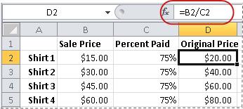
This formula divides the sale price by the percentage paid to find the original price.
Top of Page
Example 5: Calculate the difference between two numbers and show it as a percentage
Scenario For example, the earnings for your department are $2,342 in November and $2,500 in December. What is the percentage change in earnings between these two months? To do this task, use the subtraction (-) and division (/) operators in a single formula.
If B2 represents November earnings, and C2 represents December earnings, you can use the formula =(C2-B2)/ (B2) in D2 to find the difference:
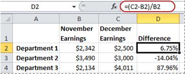
This formula divides the difference between the second and first numbers by the value of the first number to obtain the percentage change. (In the example shown here, the difference is formatted as a percentage with two decimal places.)
Top of Page
Need more help?
You can always ask an expert in the Excel Tech Community or get support in the Answers community.
Need more help?
Want more options?
Explore subscription benefits, browse training courses, learn how to secure your device, and more.
Communities help you ask and answer questions, give feedback, and hear from experts with rich knowledge.
Cell formatting in Excel allows you to represent your numbers in a variety of ways: as a date, as a percentage, as currency, and with custom formatting, even phone numbers. In today’s quick tip, we are going to show you how to quickly change a number to a percentage in Excel.
After entering a number or an array of numbers into different cells, you can format them (or format the cell before the number is entered – your preference).
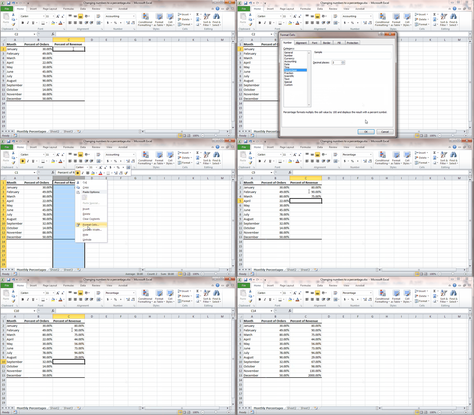
To convert the values to a percent:
- Highlight the desired cells
- Right click them
- Click the Format Cells option
- Click the Number category
- Then chose the percentage tab
This will give you the option to change how many decimals points you desire to show. After you have picked your desired decimal points, click OK and bam, it is now a percentage!
Tip: you can also click on the lettered column heading to convert the all cells within the column to your formatting preference. This is good for spreadsheets where you will be adding values over time, so that you don’t have to keep reformatting each time.
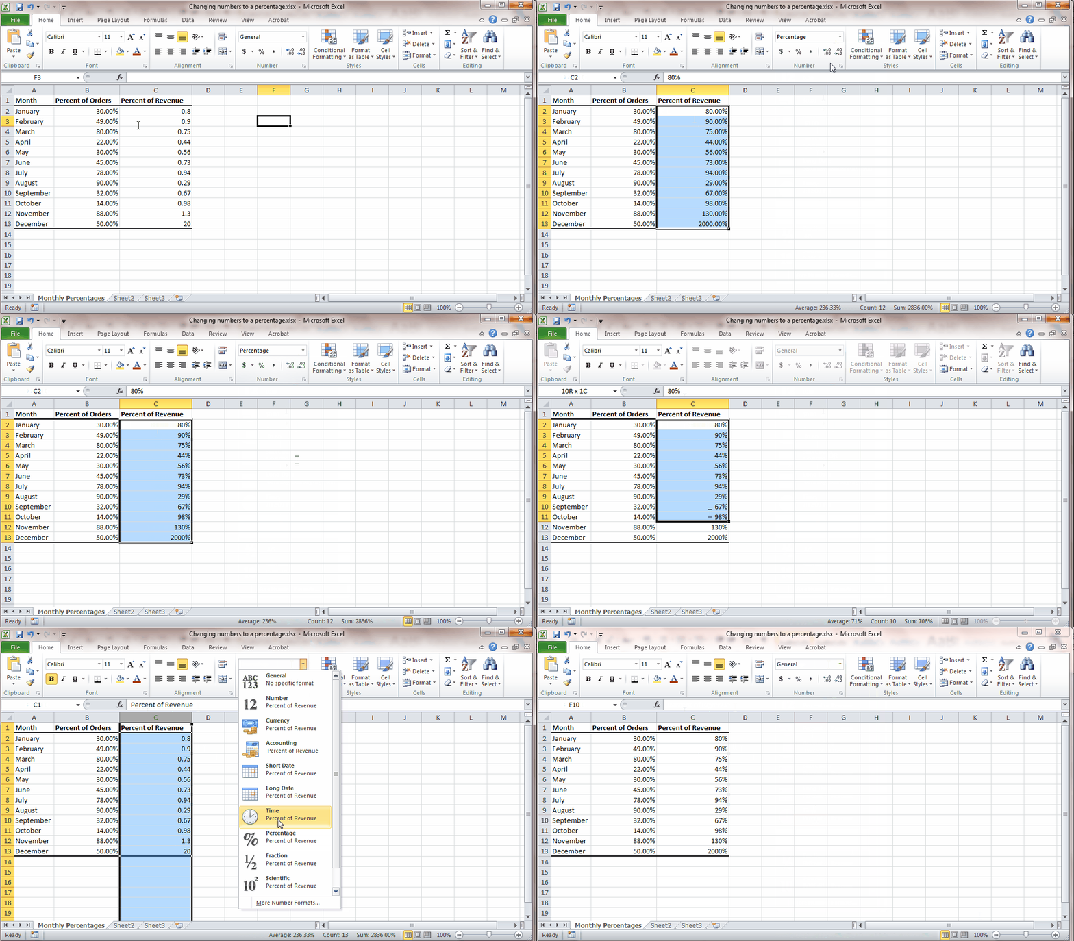
Note: if you apply the percentage format to existing numbers in a spreadsheet, excel multiplies the numbers by 100 to convert them to percentages. (If a cell contains 20, it will covert to 2000.00 %).
To format empty cells, follow the same procedure for formatting cells with existing values. Tip: you can also click on the lettered column heading to convert the all cells within the column to your formatting preference. This is good for spreadsheets where you will be adding values over time, so that you don’t have to keep reformatting each time.
As with many functions in Excel, there is another way to this as well using the Ribbon – the top toolbar in Excel.
To change numbers to a percentage in Excel using the Ribbon, click on the Ribbon, make sure you are on the home Ribbon tab. The go to the number tab and use the dropbox to select percentage. On this tab, you can also use the decimal arrow keys to select the number of decimal places you want.
We hope you found today’s quick and easy lesson on converting numbers to a percentage in Excel beneficial. Don’t forget to follow ups on Social Media and subscribe to the blog to get convenient, quick tips like this, and other great Excel training tips so that you can take the fear out of Excel.
Like Learn Excel Now? Sign up for the newsletter!
-Kevin, Learn Excel Now
Often, there are two types of percentages that one needs to calculate in Excel.
- Calculating the percentage as a proportion of a specified value (for example, if you eat 4 out of 5 mangoes, what percentage of mangoes have you eaten).
- Calculating the percentage change (YoY or MoM). This is usually used in sales reporting where the manager would want to know what’s the sales growth Year on Year, or Quarter on Quarter.
In this tutorial, I will show you the formula to calculate percentages in Excel as well as to format the cell so that the numbers show up as percentages (and not decimals).
So let’s get started!
Calculating Percentage as a Proportion
Examples of this would be to find sales coverage or project completion status.
For example, your sales manager may want to know what percentage of the total prospective customers can be reached effectively in a region.
This is known as sales coverage. Based on this, he/she can work on the sales coverage model and/or channels to reach more customers.
Here is a sales coverage example for three regions:
Looking at the example above, it would be instantly clear that the coverage is lowest in Region C, where the manager may plan some new initiatives or campaigns.
Here is the Exxcel formula to calculate the percentage in Excel:
=Effectively Reached/Total Prospective Customers
Within Excel, you can enter =B3/B2 to calculate the percentage for Region A.
Note that this would give a value in General/Number format and not in the percentage format. To make it look like a percentage, you need to apply the percentage format (shown later in this tutorial).
Calculating Percentage Change in Excel
Percentage change is widely used and monitored in various areas of business. Analysts usually talk about a company’s revenue growth or Profit growth in percentage.
Companies often track the percentage change in costs on a monthly/quarterly basis.
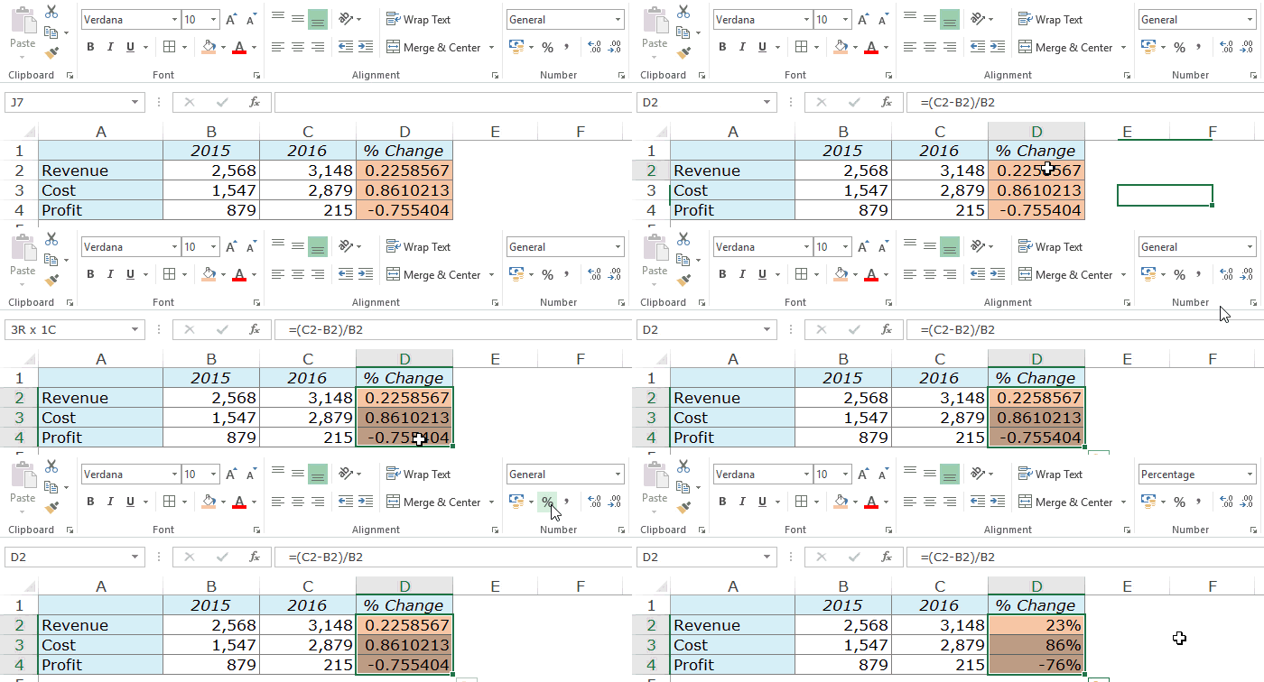
Here is a simple example of using Percentage change:
Column D has the YoY percentage change value for Revenue, Cost, and Profit. It can be easily deduced that the revenue growth was healthy but costs grew at a staggering 86.1% and lead to a decline in profits.
Here is how to calculate percentage changes in Excel:
Revenue Percentage Change = (2016 Revenue – 2015 Revenue)/2015 Revenue
In this example, the percentage formula in cell D2 is
=(C2-B2)/B2
Again, note that this would give a value in General/Number format and not in the percentage format. To make it look like a percentage, you need to apply the percentage format (shown later in this tutorial).
So let’s see how to apply the percentage formatting in Excel.
Applying Percentage Formatting in Excel
There are various ways you can apply the percentage formatting in Excel:
- Using the Keyboard Shortcut.
- Using the Ribbon.
- Using the Number Format Cells Dialog Box.
Method 1 – Using the Keyboard Shortcut
To apply the percentage format to a cell or a range of cells:
- Select the cell(s).
- Use the keyboard shortcut – Control + Shift + % (hold the Control and Shift keys and then press the % key).
Note that this applies the percentage format with no decimal places. So if you use it on 0.22587, it will make it 23%.
Method 2 – Applying Percentage Format Using the Ribbon
To apply percentage format to a cell (or a range of cells):
- Select the cell (or the range of cells).
- Go to Home –> Number –> Percent Style.
Note that this applies the percentage format with no decimal places. So if you use it on 0.22587, it will make it 23%.
If you want to have the percentage value to have decimals as well, you can use the increase decimal icon right next to the percentage icon in the ribbon.
Method 3 – Applying Percentage Format Using Format Cells Dialog Box
Using the Format Cells Dialog box gives a lot of flexibility to the user when it comes to formatting.
Here is how to apply percentage format using it:
- Select the cell (range of cells).
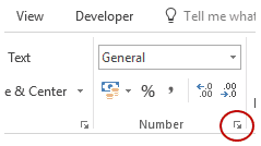
- Go to Home –> Number and click on the dialog launcher (a tilted arrow icon at the bottom right of the group). This will open the Format Cell dialog box.
- You can also use the keyboard shortcut – Control + 1 (hold the control key and press 1).
- You can also use the keyboard shortcut – Control + 1 (hold the control key and press 1).
So these are the methods you can use to calculate percentages in Excel with a formula. I also covered some methods you can use to format the number to show it as a percentage.
I hope you found this tutorial useful!
You May Also Like the Following Excel Tutorials:
- How to Calculate Weighted Average in Excel.
- How to Calculate Square Root in Excel
- How to Calculate CAGR in Excel.
- Calculating Standard Deviation in Excel.
- Excel Data Entry Tips
- Clean Data in Excel Spreadsheets
- How to Find Range in Excel
- Calculate Percentage Change in Excel (% Increase/Decrease Formula)
How to Make A Percentage Formula in Excel: Step-by-Step
We use percentages almost everywhere. For example, there’s a 50% off this weekend, monthly sales have risen by 30%, you get an annual increment of 15%, etc.
The percentage is a genius concept, and the best part – they are super easy to calculate.
This guide will help you explore a few ways to calculate and present percentages in Excel. And you’d enjoy it to the core.
Download our free sample workbook here to tag along with the guide as you continue reading.
Formula for percentage
Back to grade 4 arithmetic, here’s the formula for calculating a basic percentage.
= Value / Total Value * 100
For example, to see what percentage is 30 out of 200, you write it as shown below.
= 30 / 200 * 100
And that’s 15%.
In Microsoft Excel, there is no in-built function for calculating percentages. To reach a percentage in Excel, you need to put together the following formula
= Value / Total Value
And then format it as a percentage.
The only difference between a normal percentage formula and the Excel formula is ‘100’.
Let’s see a quick example of how this works.🙈
1. Here’s an image of the total and secured marks for some students.

Calculate the percentage marks secured by each student.
2. Activate a cell and format it as a percentage by going to Home > Number > Formats > Percentage.

4. In the same cell, now write the percentage formula as below.
= B2 / C2
Don’t forget, always start a formula with an equal sign (=) 😊

Cell B2 contains the value (the secured marks,) and Cell C2 contains the total value (the total marks).
5. Hit ‘Enter’.

Wow! Kevin scored a whopping 88%.✌
6. Drag and drop the same to all the students to calculate percentages for all.

Percentage increase in Excel
Most of the time you’d want to use Excel to calculate the percentage change between two values.
The increase or decrease percentage is calculated by dividing the difference between two numbers by the initial number (the base value).
Calculating percentage increases in Excel is super easy – see for yourself.
1. The data below shows the share prices of some companies over two years.

All the companies show an increase in the share price over the year. But what percent increase is this?
2. To calculate it, write the percentage increase formula shown below:
= (New Share Price – Old Share Price) / Old Share Price
= (C3 – B3) / B3

The above formula gives the change in share price as a percentage of the old share price.
Note the parenthesis to the subtraction function. Adding parenthesis tells Excel to perform subtraction first and the division operation last.
3. Hit ‘Enter’ and drag and drop to have the results, as below.

The shares of Company A show a percentage increase of 12%. This means the share price has increased by 12% since the last year.
If the share prices had declined over the year, the same formula would have been used to calculate the percentage decrease instead.
Showing decimals as percentages
Continuing the same example as above.
Did you see the same upon applying the percentage formula in Excel?

We applied the formula for percentage increase but all that we get is a decimal number.
Don’t fret. This is only because the ‘percentage’ format is yet not applied to the subject cell.
1. Select the cells where the decimals appear.
2. Go to Home > Number > Formats > Percentage.

You may use the shortcut to apply the percentage format by going to the Home tab > Numbers > the percentage Icon.
3. Excel changes the decimal to a percentage.

4. Maybe this percentage is not an exact round number. In most cases, percentages with zero decimal positions are rounded up / down by Excel.
5. To add decimal positions to your percentage, select the cell.
6. Go to Home > Number > Formats > More Number Formats.

7. This launches the ‘Format Cells’ Dialog box as below.
8. Go to Percentage format from the “Format Cells” dialog box.

9. Set the decimal positions to any desired number.

10. Excel adds specified decimal positions to the percentage values, as shown below.

Pro Tip!
You can also increase or decrease the decimal positions to a percentage by using the shortcut below.
Go to Home > Number > Decimal Increase / Decrease button
That’s it – Now what?
That’s all about how to calculate percentages in Excel.
Very simple but very useful. You’d need percentage calculation almost everywhere. And Excel can help you fast-forward your percentage calculations.
This guide explains how you can calculate percentage change and simple percentages in Excel. It also discusses different ways how you may format and present percentages in Excel. (With many tips to help you save time and hassle).🙌
Calculating percentages in Excel will appreciably help you. However, use it in combination with other major functions of Excel to make the best use of it.
These functions include the VLOOKUP, SUMIF, and IF functions of Excel. My 30-minute free email course takes you through these and many more functions of Excel. Sign up now.
Kasper Langmann2022-11-14T20:49:09+00:00
Page load link
The «Percentage» number format is one of the built-in number formats in Excel. In mathematics, a percentage is a number expressed as a fraction of 100. The word percent literally means «per one-hundred». For example, 65% is read as «Sixty-five percent» and is equivalent to 65/100 or 0.65.
To apply the percentage number format to a number, first select the number(s), then use any of these methods:
- Use the keyboard shortcut Control + Shift + Enter
- Select «Percentage» from the dropdown on the home tab of the ribbon
- Click the % button in the Number section on the home tab of the ribbon
- Control + 1 > Number > Percentage
Applying percentage format does not change the number, only the display of the number. In the screen above, the numbers in column B are the same as the numbers in column D.
By default, Excel will display the number with the percent sign (%) and no decimal places. To adjust this format, open the Format Cells dialog box, select Percentage, then select Custom. There you can adjust the codes in the «Type» input area. For example:
0% // default, zero decimals
0.00% // two decimal places
For more information on custom number format codes see: Custom Number Formats.
There are hundreds and hundreds of Excel sites out there. I’ve been to many and most are an exercise in frustration. Found yours today and wanted to let you know that it might be the simplest and easiest site that will get me where I want to go.
Get Training
Quick, clean, and to the point training
Learn Excel with high quality video training. Our videos are quick, clean, and to the point, so you can learn Excel in less time, and easily review key topics when needed. Each video comes with its own practice worksheet.
View Paid Training & Bundles
Skip to content
В этом коротком руководстве вы найдете много полезных сведений и узнаете, как показать результаты вычислений в процентах, как в Excel заменить число на процент по мере ввода и многое другое.
- Форматируем существующие значения — предупреждения
- Процент в пустых ячейках
- Превращаем число в процент прямо при вводе
- Советы по применению процентного формата
- Процентный формат в условном форматировании
В Microsoft Excel очень просто отображать значения в виде процентов. Чтобы применить этот формат к конкретной ячейке или к области данных, выберите их, а затем нажмите кнопку «Процентный стиль» в группе «Число» на вкладке «Главная»:
Еще более быстрый способ – нажать комбинацию клавиш Ctrl + Shift +% (Excel будет напоминать вам об этой возможности всплывающей подсказкой каждый раз, когда вы наводите курсор на кнопку «Процентный стиль»).
Хотя для форматирования чисел в виде процентов в Excel требуется всего лишь один щелчок мыши, результаты могут различаться в зависимости от того, делаете ли вы это применительно к существующим числам или к пустым ячейкам.
Форматирование существующих значений.
Когда вы применяете формат «Процент» к ячейкам, которые уже содержат числа, Excel сразу умножает эти числа на 100 и добавляет в конце знак (%). С точки зрения программы, это правильный подход, поскольку 1% – это одна сотая часть.
Однако этот способ не всегда работает корректно. Например, у вас в ячейке A1 записано число 45, и вы примените к нему процентный формат. В результате вы получите 4500%, а не 45%, как могли бы ожидать.
Возможные обходные пути:
- Перед применением процентного формата делайте предварительные вычисления. Например, если исходные числа находятся в столбце A, вы можете ввести формулу =A2/100 в B2, а затем скопировать ее вниз по столбцу. Затем выделите весь столбец B и примните к нему процентный стиль. Вы получите примерно такой результат:
Теперь вы можете заменить формулы значениями в столбце B, скопировать их обратно в столбец A и удалить столбец B, если он вам больше не нужен. Для этого используйте Специальная вставка – Значения. Быстрые клавиши: сначала Ctrl+C, затем для вставки Ctrl+Alt+V.
- Если вы хотите применить процентное форматирование только к нескольким числам, вы можете ввести число в десятичной форме прямо в ячейку. Например, чтобы в ячейке A2 было 15%, введите 0,15 и затем примените формат.
Применение процентного формата к пустым ячейкам
Microsoft Excel ведет себя по-другому, когда вы вводите числа в пустые ячейки, предварительно отформатированные как процент:
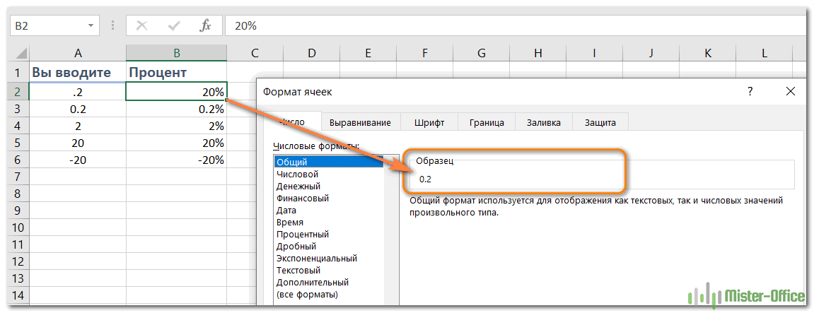
- Любое число, равное или больше 1, автоматически преобразуется в процент. Например, 2 превращается в 2%, 20 — в 20%, дробное число 7,15 в 7,15% и так далее.
- Числа меньше 1 без предшествующего нуля в целой части автоматически умножаются на 100. Например, если вы введете .2 в ячейку в процентном формате, вы увидите в этой ячейке 20%. Однако, если вы запишете 0.2 в этой же ячейке, то 0.2% будет отображаться именно так, как и должно быть.
Отображение чисел в процентах при их вводе
Если вы введете 20% (со знаком %) прямо в ячейку, Эксель поймет, что именно вы вводите, и автоматически применит к ней процентное форматирование.
Важное замечание. Применяя формат процента, имейте в виду, что это не более чем визуальное представление реального значения, хранящегося в ячейке. Базовое значение всегда хранится в десятичном виде.
Другими словами, 20% сохраняется как 0,2, 2% на самом деле 0,02, 0,2% равно 0,002 и т.д. При выполнении вычислений Excel всегда имеет дело с десятичными значениями. Помните об этом факте, когда ссылаетесь на ячейки с процентным форматом в формулах.
Чтобы увидеть реальное значение, скрытое под форматированием, щелкните ячейку правой кнопкой мыши, выберите Формат ячеек (или нажмите Ctrl + 1) и посмотрите в поле Образец на вкладке Число.
Советы по отображению процентов в Excel
Отображение процентов в Excel кажется одной из самых простых задач, верно? Но опытные пользователи знают, что путь к цели почти никогда не бывает гладким 
1. Десятичные знаки.
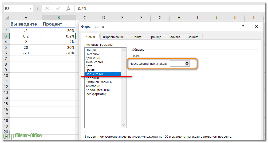
При применении этого форматирования к числам Excel отображает их округлёнными без десятичных знаков. Это может вызвать некоторую путаницу. Например, мы выше рассматривали, как установили процентный формат в пустой ячейке, а затем вводили в нее 0.2. Что мы там видели? В моем случае я увидел 0%, хотя я точно знаю, что это должно быть 0,2%. И к этому нужно быть готовым.
Чтобы увидеть фактическое значение вместо округленного числа, вам просто нужно увеличить количество отображаемых десятичных разрядов. Для этого откройте диалоговое окно Формат ячеек, нажав Ctrl + 1. Убедитесь, что выбран числовой формат «Процент», и укажите желаемое количество разрядов в поле «Десятичные знаки».
Когда закончите, нажмите кнопку ОК, чтобы сохранить настройки.
Кроме того, вы можете управлять количеством отображаемых десятичных знаков, щелкнув на ленте значки «Увеличить разрядность» или «Уменьшить разрядность»:
2. Отрицательные числа.
Если вы хотите выделить отрицательные проценты особым способом, например красным цветом, вы можете создать собственный числовой формат. Откройте диалоговое окно Формат ячеек и перейдите на раздел > Все форматы. Введите один из ниже форматов в поле Тип:
0.00%; [Красный] -0.00% – закрасить отрицательные числа красным цветом и отображать 2 десятичных знака.
0%; [Красный] -0% – изобразить отрицательные значения красным без десятичных знаков.
Как выделить отрицательные проценты с помощью условного форматирования.
По сравнению с предыдущим методом, условное форматирование Excel более универсально и позволяет отображать отрицательные проценты, например уменьшение на сколько-то процентов, в любом формате по вашему выбору.
Самый быстрый способ создать правило условного форматирования для отрицательных чисел – это щелкнуть Условное форматирование> Правила выделения ячеек> Меньше чем и поставить 0 в поле «Форматировать ячейки меньше»:
Затем вы выбираете один из вариантов форматирования из раскрывающегося списка справа или щелкаете Пользовательский. в конце списка, чтобы настроить свой вариант.
Дополнительные сведения о создании правил условного форматирования см. в разделе Как использовать условное форматирование в Excel .
Вот как можно работать с процентным форматом в Excel. Надеюсь, эти знания помогут вам избежать головной боли в будущем. Следите за обновлениями и благодарим за чтение!
 Формат времени в Excel — Вы узнаете об особенностях формата времени Excel, как записать его в часах, минутах или секундах, как перевести в число или текст, а также о том, как добавить время с помощью…
  Как умножить число на процент и прибавить проценты — Ранее мы уже научились считать проценты в Excel. Рассмотрим несколько случаев, когда известная нам величина процента помогает рассчитать различные числовые значения. Чему равен процент от числаКак умножить число на процентКак…
  Как считать проценты в Excel — примеры формул — В этом руководстве вы познакомитесь с быстрым способом расчета процентов в Excel, найдете базовую формулу процента и еще несколько формул для расчета процентного изменения, процента от общей суммы и т.д.…
  Как сделать пользовательский числовой формат в Excel — В этом руководстве объясняются основы форматирования чисел в Excel и предоставляется подробное руководство по созданию настраиваемого пользователем формата. Вы узнаете, как отображать нужное количество десятичных знаков, изменять выравнивание или цвет шрифта,…
  7 способов поменять формат ячеек в Excel — Мы рассмотрим, какие форматы данных используются в Excel. Кроме того, расскажем, как можно быстро изменять внешний вид ячеек самыми различными способами. Когда дело доходит до форматирования ячеек в Excel, большинство…
  Как удалить формат ячеек в Excel — В этом коротком руководстве показано несколько быстрых способов очистки форматирования в Excel и объясняется, как удалить форматы в выбранных ячейках. Самый очевидный способ сделать часть информации более заметной — это…
We often have to work with percentages in our day-to-day work and our everyday life. Excel makes this task easier by automatically applying basic or advanced formulas that allow you to calculate percentages directly in your spreadsheets. We’ll show you how to use the most important formulas in Excel to calculate percentages of totals or percentage changes such as growth and decline. You’ll also learn how to calculate proportions and totals based on percentages and how to increase and decrease numbers by percentage.
Contents
- Calculating percentages in Excel – the basics
- Calculating percentages in Excel – formulas and formatting
- Adding percentage formatting in Excel
- Adjusting percentage formatting in Excel
- Calculating the percentage of a total in Excel
- Calculating the percentage of a total at the end of an Excel table
- Calculating percentages of a total from different rows
- Formula for calculating a percentage change in Excel
- Calculating the percentage of change between two columns
- Calculating the percentage of growth between two rows
- Calculating the proportion and the total based on a percentage in Excel
- Calculating the proportion based on the total and based on percentages
- Calculating the total based on the proportion and percentage
- Increasing and decreasing numbers by a percentage in Excel
$1 Domain Names
Register great TLDs for less than $1 for the first year.
Why wait? Grab your favorite domain name today!
Matching email
SSL certificate
24/7/365 support
Calculating percentages in Excel – the basics
In this article, we’ll give you an overview of the most important methods for calculating percentages in Excel and show you the most important formulas for doing percentages.
Tip
Microsoft Excel can help you with many basic and advanced calculations in your day-to-day work. Learn more about the SUM function in Excel if you want to easily add groups of numbers.
The word “percent” is of Latin origin and means “by a hundred”. In other words, you calculate a percentage by dividing the numerator of a fraction by the denominator and multiplying the result by 100. The basic formula for calculating apercentage looks like this:
(Part/Total)*100=PercentageFor example, if you sell a product for $14 that costs $10.50 to manufacture, the manufacturing cost is 75 percent of the total price. We often use this formula to calculate percentages in our everyday lives. However, with Excel, calculating percentages is even easier because the spreadsheet application automatically performs several steps in the background.
Tip
Organize your data in Excel, create spreadsheets, and calculate your expenses, profits, and much more. Get the spreadsheet program as part of the Microsoft 365 package directly from IONOS and get optimum round-the-clock support for Microsoft Excel and other Office products.
Calculating percentages in Excel – formulas and formatting
When you calculate percentages in Excel, you’ll save yourself steps like multiplying by 100 because the application automatically handles the formatting for you once you apply the percent format (see below for more information). The formula for calculating percentages in Excel is as follows:
Let’s look at a practical example of how percentages are calculated in Excel: A retailer uses a spreadsheet of purchased and sold products in order to keep track of inventory. The number of products that the retailer buys is in column B and the number of products that the retailer sells in is column C. To calculate the percentages in column D of the Excel spreadsheet, enter the following formula (and then press Enter):
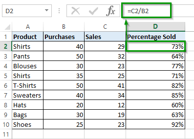
You can easily apply the formula to subsequent rows by double-clicking the bottom right corner of the cell (in this case: D2). Excel also automatically adds the formula as you enter more data in columns B and C.
Adding percentage formatting in Excel
However, the results may not look quite right at first: Instead of percentages, you’ll see decimal numbers in your Excel spreadsheet.
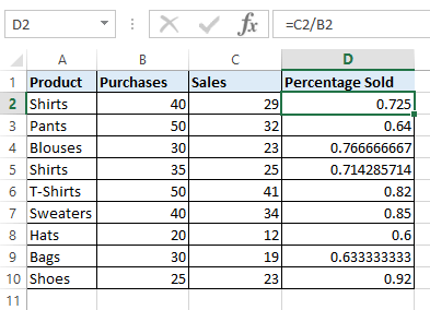
If you want Excel to automatically add the percent sign and round up to the percentage using the formatting, you have to adjust the following settings first: To quickly change the cell format to show values as percentages in Excel, go to the “Number” group (between “Alignment” and “Styles”) on the “Home” tab. Once there, simply click the percent sign to select the percent format – either for a single cell, a range of cells or an entire column or row. In this case, we calculated percentages in column D of our Excel spreadsheet by selecting the appropriate cells beforehand:
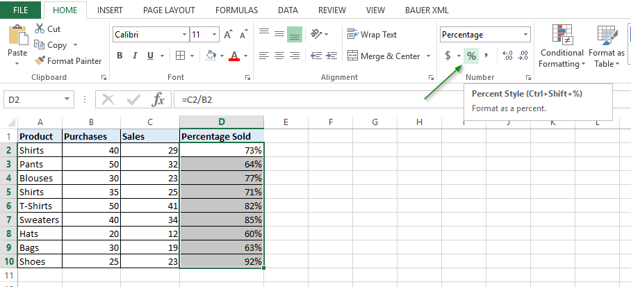
Alternatively, you can use the keyboard shortcut Ctrl + Shift + % (as shown in the screenshot above) to enable the percentage format.
Adjusting percentage formatting in Excel
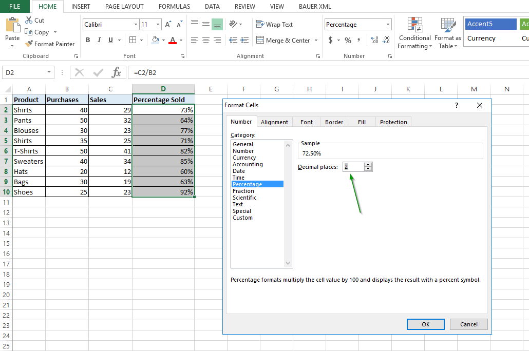
If you follow the steps above, percentages are displayed without decimal places according to the default settings in Excel. However, you can change the percentage formatting in Excel simply by clicking the little arrow icon at the bottom right in the “Number” group. Alternatively, you can select a cell and right-click it to display the “Format cells” dialog box.
To adjust the percentages in Excel, you can then specify the number of decimal places you want to display. For example, to display two digits after the decimal point, select “2”. Then click OK.
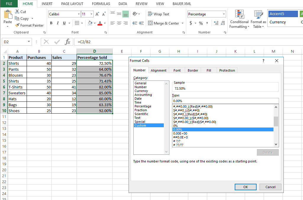
Alternatively, you can choose the “Custom” category in the same dialog box to specify percentages either without a decimal place or with two decimal places.
Note
Formats in Excel not only help you calculate percentages; you can also use them for many other processes and tasks. For example, in another article we explain how to calculate time in Excel.
Calculating the percentage of a total in Excel
In the examples above, we calculated percentages of a total. The purchases and sales are the total and the sales are the percentages. However, we can also use Excel to do more complicated calculations for finding the percentages of a total.
Calculating the percentage of a total at the end of an Excel table
Let’s say the retailer in the example above now wants to know how many products they purchased in total and what percentage of the total purchase amount is attributed to each product. Excel works out the percentage of the total that each amount represents. However, first we have to determine the total quantity of all products in cell B11. In the column to the right, we use Excel to find out what percentage of the total each product represents. To do this, we enter the following values in cell C2 or select these values with the mouse button:
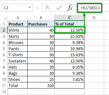
The $ signs create an absolute reference to cell B11. This means that the value does not change even if the other values change according to the spreadsheet. For example, “=B3/$B$11” appears in cell C3 after the formula from cell C2 is automatically applied. Without the absolute value, which is indicated by the dollar sign, “=B3/B12” would appear in this cell and the example formula would not calculate any percentages because cell B12 is empty.
Note
You can also define a cell as an absolute value by pressing the [F4] key on your keyboard after you have selected the cell with the mouse or entered it manually.
Calculating percentages of a total from different rows
Now let’s say the retailer has multiple rows for the same product and wants to use Excel to find out what percentage of the total that product represents. In this case, you can use the SUMIF formula, which automatically adds all values that match the criteria you have selected. Combined with the SUMIF formula, the complete formula for calculating percentages in Excel looks like this:
=SUMIF(range,criteria,sum_range)/totalIn our example, we entered the criteria “Pants” in cell E1. The values that we want to add are in column B and the product names for automated selection are in column A. The corresponding formula in Excel is as follows:
=SUMIF(A2:B10,E1,B2:B10)/$B$11Here’s how it looks in the Excel spreadsheet:
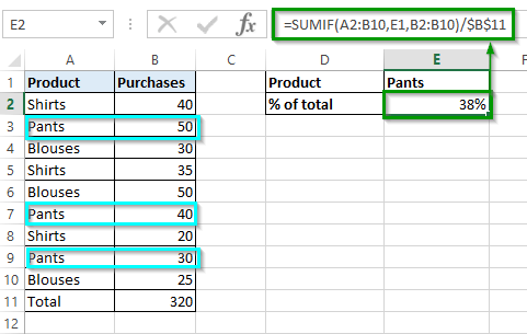
Instead of specifying your criteria in a cell of your Excel spreadsheet, you can type it directly into your formula, which then reads “SUMIF(A2:B10,»Pants»,B2:B10)/$B$11”. You can also use parentheses to work with multiple SUMIF functions, for example, to calculate percentages of multiple products in Excel:
=(SUMIF(A2:B10;"Pants",B2:B10)+SUMIF(A2:B10,"Shirts",B2:B10))/$B$11))Formula for calculating a percentage change in Excel
The percentage of change or percentage of growth is probably one of the formulas that you’ll use most often when you calculate percentages in Excel. Simply use the following formula to calculate the change between the original value A and the value B:
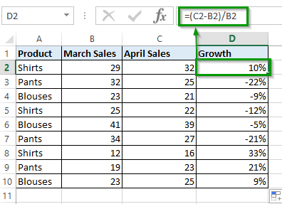
Percentage change=(B-A)/AThe original value A represents the value before the change. For example, if you compare sales between the two months of March and April, the number of sales in March would be the original value A and sales in April would be B. The following two examples illustrate how to calculate the percentage of growth using this formula.
Calculating the percentage of change between two columns
The retailer in our example entered the sales from March in column B and the sales from April in column C. The retailer then enters the following formula in column D to calculate the percentage of growth:
Note
Don’t forget: After this step, you have to format the cells in column D as percentages so that the result is displayed correctly.
Calculating the percentage of growth between two rows
You may want to keep track of total monthly sales in a spreadsheet. In this case, you can calculate the percentage of growth between two rows so that you can easily see month-over-month changes in sales. In the example, we enter all monthly sales in column B and calculate the growth in column C. Start with the sales from January in cell B2 and determine the percentage of growth for February in cell C3. To do this, enter the following formula in cell C3:
Then apply the formula to the subsequent rows (starting with C4). In your Excel spreadsheet, you can see the percentage of growth as follows:
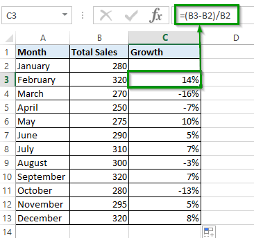
When you calculate the percentage of growth, be sure to leave the first row blank because it is not being used in the comparison. In this example, you are not comparing January to the prior month.
You can also calculate the percentage of growth in Excel in comparison to a static value that does not change. To do this, simply enter the absolute reference to the cell by pressing the F4 key and adding the $ sign as explained above.
Calculating the proportion and the total based on a percentage in Excel
Just as you can use Excel formulas to calculate percentages based on two values, A and B, you can also calculate a total or the proportions of a totalbased on a percentage.
Calculating the proportion based on the total and based on percentages
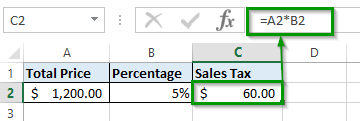
Let’s say you buy new IT equipment for your company and the total price is $1,200. This includes sales tax, which may be tax-deductible. Sales tax varies from state to state, so for the sake of illustration let’s assume that you live in Wisconsin, where sales tax is 5%. For this purpose, you simply calculate the amount of sales tax based on the percentage. In the following example, the total price is in cell A2 and the percentage is in cell B2. You need to calculate the absolute value of the sales in cell C2. The appropriate formula is:
The result: The purchase price includes $60 of sales tax.
Tip
If you don’t want to enter the percentage in a separate cell, you can also integrate it directly into the formula. Enter either “=A2*5%” or “=A2*0.05”.
Calculating the total based on the proportion and percentage
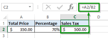
Excel also allows you to calculate a total based on the proportion and percentage. For example, let’s say you attend a multi-day workshop in another city. As a workshop attendee, you receive a special discount and pay only 70 percent of the price of your hotel room as part of your all-inclusive accommodations. You are charged $350 and are curious how expensive your stay would have been without the discount.
Enter the amount you paid in cell A2 and the percentage in cell B2. In cell C2, enter the formula for calculating the total price based on percentages. Divide your amount by the percentage:
If you entered everything correctly, you’ll see that the hotel price would have been $500 without the discount:
Increasing and decreasing numbers by a percentage in Excel
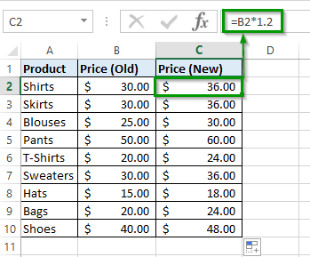
You can also use percentages to increase and decrease numbers in Excel. This is especially useful for our retailer in the previous examples. For example, if the retailer wants to increase all prices by 20 percent to compensate for increased expenses, they can use the following formula:
The retailer can then reduce the prices again during the end-of-season sale. Note that Excel also recognizes the decimal notation when calculating the percentage:
In the example, a price increase looks like this: Column A shows the product type and column B shows the current price. To calculate the new price in column C, the retailer uses the following formula:
The retailer now sees the new prices, which are 20 percent higher, in column C:
