Excel format as datetime

When you type a date or time in a cell, it appears in a default date and time format. This default format is based on the regional date and time settings that are specified in Control Panel, and changes when you adjust those settings in Control Panel. You can display numbers in several other date and time formats, most of which are not affected by Control Panel settings.

In this article

• Display numbers as dates or times

• Create a custom date or time format

• Tips for displaying dates or times

Display numbers as dates or times

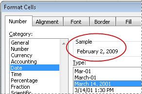
You can format dates and times as you type. For example, if you type 2/2 in a cell, Excel automatically interprets this as a date and displays 2-Feb in the cell. If this isn’t what you want—for example, if you would rather show February 2, 2009 or 2/2/09 in the cell—you can choose a different date format in the Format Cells dialog box, as explained in the following procedure. Similarly, if you type 9:30 a or 9:30 p in a cell, Excel will interpret this as a time and display 9:30 AM or 9:30 PM. Again, you can customize the way the time appears in the Format Cells dialog box.

1. On the Home tab, in the Number group, click the Dialog Box Launcher next to Number.

   

   You can also press CTRL+1 to open the Format Cells dialog box.

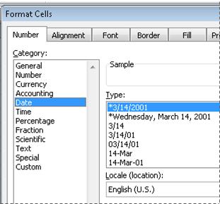
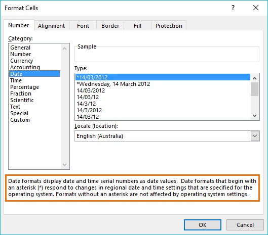
2. In the Category list, click Date or Time.

   

3. In the Type list, click the date or time format that you want to use.

   Note: Date and time formats that begin with an asterisk (*) respond to changes in regional date and time settings that are specified in Control Panel. Formats without an asterisk are not affected by Control Panel settings.

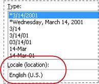
4. To display dates and times in the format of other languages, click the language setting that you want in the Locale (location) box.

   

   The number in the active cell of the selection on the worksheet appears in the Sample box so that you can preview the number formatting options that you selected.

   

Top of Page

Create a custom date or time format

1. On the Home tab, click the Dialog Box Launcher next to Number.

   

   You can also press CTRL+1 to open the Format Cells dialog box.

2. In the Category box, click Date or Time, and then choose the number format that is closest in style to the one you want to create. (When creating custom number formats, it’s easier to start from an existing format than it is to start from scratch.)

3. In the Category box, click Custom. In the Type box, you should see the format code matching the date or time format you selected in the step 3. The built-in date or time format can’t be changed or deleted, so don’t worry about overwriting it.

4. In the Type box, make the necessary changes to the format. You can use any of the codes in the following tables:

   Days, months, and years    

To display	Use this code
Months as 1–12	m
Months as 01–12	mm
Months as Jan–Dec	mmm
Months as January–December	mmmm
Months as the first letter of the month	mmmmm
Days as 1–31	d
Days as 01–31	dd
Days as Sun–Sat	ddd
Days as Sunday–Saturday	dddd
Years as 00–99	yy
Years as 1900–9999	yyyy

If you use «m» immediately after the «h» or «hh» code or immediately before the «ss» code, Excel displays minutes instead of the month.

Hours, minutes, and seconds

To display	Use this code
Hours as 0–23	h
Hours as 00–23	hh
Minutes as 0–59	m
Minutes as 00–59	mm
Seconds as 0–59	s
Seconds as 00–59	ss
Hours as 4 AM	h AM/PM
Time as 4:36 PM	h:mm AM/PM
Time as 4:36:03 P	h:mm:ss A/P
Elapsed time in hours; for example, 25.02	[h]:mm
Elapsed time in minutes; for example, 63:46	[mm]:ss
Elapsed time in seconds	[ss]
Fractions of a second	h:mm:ss.00

AM and PM     If the format contains an AM or PM, the hour is based on the 12-hour clock, where «AM» or «A» indicates times from midnight until noon and «PM» or «P» indicates times from noon until midnight. Otherwise, the hour is based on the 24-hour clock. The «m» or «mm» code must appear immediately after the «h» or «hh» code or immediately before the «ss» code; otherwise, Excel displays the month instead of minutes.

Creating custom number formats can be tricky if you haven’t done it before. For more information about how to create custom number formats, see Create or delete a custom number format.

Top of Page

Tips for displaying dates or times

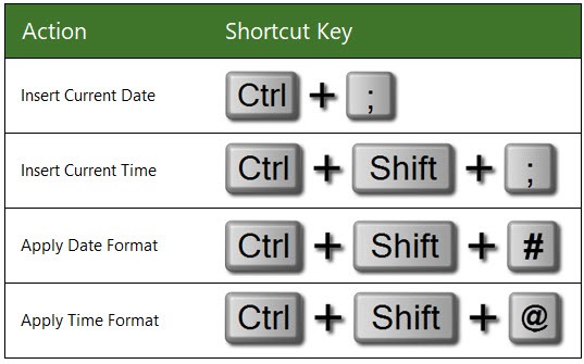
• To quickly use the default date or time format, click the cell that contains the date or time, and then press CTRL+SHIFT+# or CTRL+SHIFT+@.

• If a cell displays ##### after you apply date or time formatting to it, the cell probably isn’t wide enough to display the data. To expand the column width, double-click the right boundary of the column containing the cells. This automatically resizes the column to fit the number. You can also drag the right boundary until the columns are the size you want.

• When you try to undo a date or time format by selecting General in the Category list, Excel displays a number code. When you enter a date or time again, Excel displays the default date or time format. To enter a specific date or time format, such as January 2010, you can format it as text by selecting Text in the Category list.

• To quickly enter the current date in your worksheet, select any empty cell, and then press CTRL+; (semicolon), and then press ENTER, if necessary. To insert a date that will update to the current date each time you reopen a worksheet or recalculate a formula, type =TODAY() in an empty cell, and then press ENTER.

Need more help?

You can always ask an expert in the Excel Tech Community or get support in the Answers community.

So I’ve been battling with this issue all day.

Basically I have it now sorted and part of the solution was a code that Excel itself generated which is:

[$-en-AU]yyyy-mm-dd hh:mm

So, in the first instance,

• in a new spreadsheet, type your entry in as per usual, eg: 2026-01-31 10:00
• set the format of the cell to «custom» and use the above formula, ie
  [$-en-AU]yyyy-mm-dd hh:mm
• Hit enter and Bob’s your uncle!

Then save it as a CSV file, then close it and re-open it to check Excel hasn’t changed the date format.

The weird thing is if it does work (and I’ve re-tried it a few times successfully), when you check the format of the cell you’ve created, it’s changed the format to «General».

But seriously who cares. As long as it works!!

You can then copy and paste the cell and use it wherever you want!!

I hope this solution works for you!!

Regards

Richard

It is common to import data from other sources in Excel and it is also common to not get properly formatted data. For example, most of the time when we get data from other sources the date, time and numeric values are in text format. They need to be converted in the proper format. It is easy to convert numbers into excel numbers. But converting string into excel datetime may need a little bit of effort. 

In this article, we will learn how you can convert text formatted date and time in excel date and time.

Generic Formula

Datetime_string: This is the reference of the string that contains the date and time.

The main functions in this generic formula are DATEVALUE and TIMEVALUE. Other functions are used to extract date string and time string if they are combined into one string. And yes, the cell that contains this formula should be formatted into datetime format otherwise you will see serial numbers that may confuse you.

Let’s see some examples to make things clear.

Example: Convert Imported Date and Time into Excel Datetime

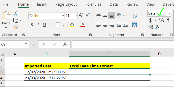
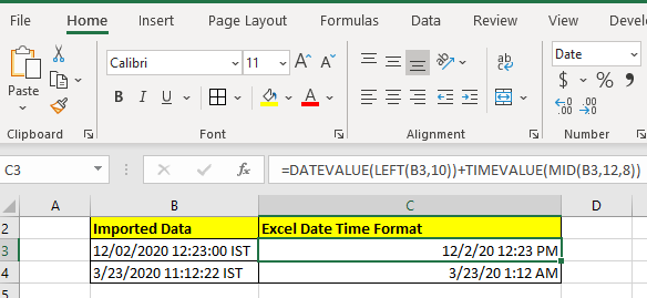
Here we have date and time combined into one string. We need to extract date and time separately and convert them into excel datetime.

Note that I have formatted C3 as a date so that the results I get are converted into dates and I don’t see a fractional number. (Secrets of excel date and time).

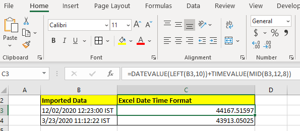
So let’s write the formula:

And it returns the date and time that excel considers as datetime, not string.

If you don’t change the cell formatting, this is what your result will look like.

This isn’t wrong. It is the serial number that represents that date and time. If you don’t know how the date and time are perceived by Excel, you can get complete clarity here.

How does it work?

This is simple. We use extraction techniques to extract date and time strings. Here we have LEFT(B3,10). This returns 10 characters from the left of the string in B3. Which is «12/02/2020». Now this string is supplied to the DATEVALUE function. And DATEVALUE converts the date string into its value. Hence we get 44167.

Similarly, we get time value using  MID function (for extraction) and TIMEVALUE function.

The MID function returns 8 characters from the 12th  position in string. Which is «12:23:00». This string is supplied to TIMEVALUE function that returns .51597.

Finally we add these numbers up. This gives us the number 44167.51597. When we convert the cell formatting to MM/DD/YYYY HH:MM AM/PM format we get the exact datetime.

In the above example, we had date and time concatenated together as a string. If you just have date as string without any extra text or string, you can use the DATEVALUE function alone to get the Date converted into excel date.

If you just have time as a string use the TIMEVALUE function

You can read about these functions by clicking on the function name in the formula.

So yeah guys, this is how you convert a date and time string into excel date time value. I hope this was helpful. If you have any doubts regarding this article or have any other query related Excel/VBA, ask me in the comment section below. I will be happy to help you.

Related Articles:

Convert Date and Time from GMT to CST : While working on Excel reports and Excel dashboards in Microsoft Excel, we need to convert Date and Time. In addition, we need to get the difference in timings in Microsoft Excel. 

How to Convert Time to Decimal in Excel : We need to convert the time figures into decimals using a spreadsheet in Excel 2016. We can manipulate time in excel 2010, 2013 and 2016 using the function CONVERT, HOUR and MINUTE.

How to Convert date to text in Excel : In this article we learned how to convert text into date, but how do you convert an excel date into text. To convert an excel date into text we have a few techniques.

Converting Month Name to a Number in Microsoft Excel : When it comes to reports numbers are better than text. In Excel if you want to convert month names into numbers (1-12). Using the function DATEVALUE and MONTH you can easily convert months into numbers.

Excel convert decimal Seconds into time format : As we know, time in excel is treated as numbers. Hours, Minutes, and Seconds are treated as decimal numbers. So when we have seconds as numbers, how do we convert them into time format? This article got it covered.

Popular Articles:

50 Excel Shortcuts to Increase Your Productivity | Get faster at your task. These 50 shortcuts will make you work even faster on Excel.

How to use Excel VLOOKUP Function| This is one of the most used and popular functions of excel that is used to look up value from different ranges and sheets. 

How to use the Excel COUNTIF Function| Count values with conditions using this amazing function. You don’t need to filter your data to count specific values. Countif function is essential to prepare your dashboard.

How to Use the SUMIF Function in Excel | This is another dashboard essential function. This helps you sum up values on specific conditions.

The objective of this post is to teach you how Excel handles date and time and provide you with all the tools you will need.

It’s designed to be read in conjunction with the accompanying Excel file, which you can download below.

Download the Files

Regional Settings

When reading this post keep in mind that my regional settings format dates as dd/mm/yyyy and so the screenshots throughout this post are in this format. However, if you open the accompanying Excel file you may see some dates have switched to match your regional settings, which may be different to mine e.g. mm/dd/yyyy.

Dates and times with a format that begins with an asterisk (*) automatically update based on your PC’s regional settings. You can see an example in the Format Cells dialog box below:

Ok, let’s crack on.

Excel Date and Time 101

Excel stores dates and time as a number known as the date serial number, or date-time serial number.

When you look at a date in Excel it’s actually a regular number that has been formatted to look like a date. If you change the cell format to ‘General’ you’ll see the underlying date serial number.

The integer portion of the date serial number represents the day, and the decimal portion is the time. Dates start from 1st January 1900 i.e. 1/1/1900 has a date serial number of 1.

Caution! Excel dates after 28th February 1900 are actually one day out. Excel behaves as though the date 29th February 1900 existed, which it didn’t.

Microsoft intentionally included this bug in Excel so that it would remain compatible with the spreadsheet program that had the majority market share at the time; Lotus 1-2-3.

Lotus 1-2-3 was incorrectly programmed as though 1900 was a leap year. This isn’t a problem as long as all your dates are later than 1st March 1900.

Excel gives each date a numeric value starting at 1^st January 1900. 1^st January 1900 has a numeric value of 1, the 2^nd January 1900 has a numeric value of 2 and so on. These are called ‘date serial numbers’, and they enable us to do math calculations and use dates in formulas.

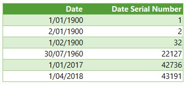
The Date Serial Number column displays the Date column values in their date serial number equivalent.

e.g. 1/1/2017 has a date serial number of 42736. i.e. 1^st January 2017 is 42,736 days since 31st December 1899.

Tip: format the date serial number column as a Date and you’ll see they look the same as the Date column values.

Time

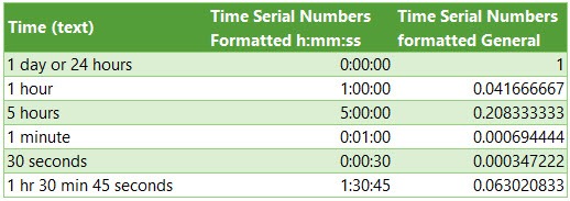
Times also use a serial number format and are represented as decimal fractions.

Hours: since 24 hours = 1 day, we can infer that 24 hours has a time serial number of 1, which can be formatted as time to display 24:00 or 12:00 AM or 0:00. Whereas 12 hours or the time 12:00 has a value of 0.50 because it is half of 24 hours or half of a day, and 1 hour is 0.41666′ because it’s 1/24 of a day.

Minutes: since 1 hour is 1/24 of a day, and 1 minute is 1/60 of an hour, we can also say that 1 minute is 1/1440 of a day, or its time serial number is 0.00069444′

Seconds: since a second is 1/60 of a minute, which is 1/60 of an hour, which is 1/24 of a day. We can also say one second is 1/86400 of a day or in time serial number form it’s 0.0000115740740740741…

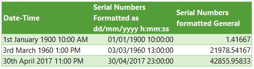
Date & Time Together

Now that we know how dates and times are stored we can put them together — ddddd.tttttt

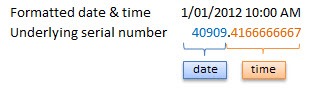
For example, the date and time of 1^st January 2012 10:00:00 AM has a date-time serial value of 40909.4166666667

40909 being the serial value representing the date 1^st January 2012, and .4166666667 being the decimal value for the time 10:00 AM and 00 seconds.

More examples below.

Entering Dates & Times in Excel

Entering Dates

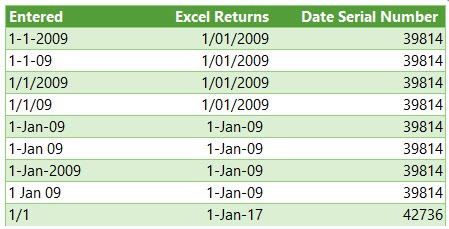
You can type in various configurations of a date and Excel will automatically recognise it as a date and upon pressing ENTER it will convert it to a date serial number and apply a date format on the cell.

For example, try typing (or even copy and paste) the following dates into an empty cell:

1-1-2009

1-1-09

1/1/2009

1/1/09

1-Jan-09

1-Jan 09

1-Jan-2009

1 Jan 09

1/1

 

You can see in the table above that entering numbers that look like dates and are separated by a forward slash or hyphen will be recognised as a date. Even typing in a date with the month name gets converted to a date.

However, dates separated with a period like this 1.1.2009, or with spaces between numbers like this 01 01 2009, will end up as text, not a date. Gotta have some limits!

Tip: Dates that display ##### in a cell usually indicate that the column is simply not wide enough to display it.

However, if you make the cell really wide and it still displays ##### then this indicates that the date is a negative value and Excel can’t display negative dates.

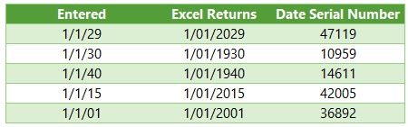
Entering Dates with Two Digit Years

When you enter a date with two digits for the year e.g. 1/1/09, Excel has to decide if you mean 2009 or 1909.

It goes by the rule that dates with years 29 or before, are treated as 20xx and dates with the year 30 or older are treated as 19xx. See examples below.

Tip: You can enter the day and month portions of a date and Excel will insert the year based on your computer’s clock. Nice to know for data entry.

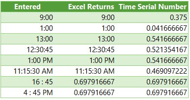
Entering Time

When you enter time you must follow a strict format of at least h:mm. i.e. the hour and minutes are separated by a colon with no spaces either side. Entering the h:mm components will result in a time formatted in military time e.g. 2:00 PM is 14:00 in military time.

If you enter a time that includes a seconds component e.g. 3:15:40, Excel will automatically format the cell in h:mm:ss.

If you want the time to be formatted with AM/PM you can simply enter a space after the time and then type AM or PM, or apply the number format to the cell later. Here are some examples:

Entering Dates & Time Together

Now that we know how to enter dates and time separately we can put them together to enter a date and time in the same cell.

You can even enter time then date and Excel will fix the order for you.

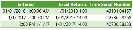
You’ll find that even if you enter AM/PM, that Excel will convert it to military time by default. You can override this with a custom number format. More on that later.

Simple Date & Time Math

Now that we understand that Excel stores dates and time as serial numbers, you’ll see how logical it is to perform math operations on these values. We’ll look at some simple examples here and tackle the more complex scenarios later when we look at Date and Time Functions.

Adding/Subtracting Days from Dates

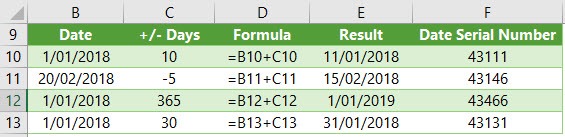
Tip: you can also add/subtract the days directly in the formula e.g. =B10+10 or =B11-5 Although, it’s better to place the values you’re adjusting by in their own cell or a named range.

Subtracting Dates from one another

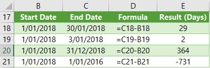
Tip: format the cell to General or Number to see the number of days between two dates.

Note: the ‘result’ is exclusive of the start day i.e. it assumes the start day is at the end of that day.

Adding Times to one another

The time being added is input as a time serial number. Notice there are no negative times in the table below. Remember we can’t display negative times. Instead we need to use the math operator to tell Excel to subtract time.  See examples below.

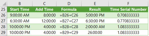
Note: Times that roll over to the next day result in a time-date serial number >= 1. Cell E28 actually contains a time-serial number of 1.08333′, but since the cell is formatted to display time formatted as h:mm:ss, only the time portion is visible.

If you want to show the cumulative time (like cell E29) then you need to surround the ‘h’ part of the time format in square brackets like so: [h]:mm:ss

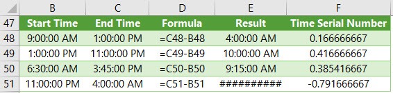
Subtracting Time from Times

Notice the last result in the table below shows ######, this is because it results in a negative time and Excel can’t display that, but notice it can return a negative time serial number. More on how to solve this later.

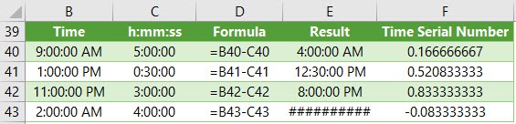
Subtracting Times from one another

Again, here the last result shows ###### because it results in a negative time.

Excel Date and Time Shortcuts

‘Good to Know’ Stuff about Excel Date and Time

— Dates prior to 1st January 1900 are not recognised in Excel.

— A negative date will display in the cell as #######

— Times stored without a date effectively inherit the date 0 Jan 1900 i.e. the month is Jan and the year 1900 and the day is zero. Remember, there are no dates prior to 1/1/1900 from Excel’s perspective. This means that times stored without a date e.g. 0.50 for 12:00 PM is the equivalent of 0 Jan 1900 12:00 PM.

This is important because if you try to take 14 hours from 12 hours (without a date) you’ll get the dreaded ###### display in the cell, because negative dates and times cannot be displayed. We’ll cover workarounds for this later, but for now keep in mind that math on dates and time that result in negative date-time serial numbers cannot be formatted as a date.

Date Modes

— Excel actually has two date modes. The other mode is called 1904 Date System and is used for compatibility with Excel 2008 for Mac and earlier Mac versions. You can change the date system in the Advanced Options.

In the 1904 date system dates are calculated using 1st January 1904 as the starting point. The difference between the two date systems is 1,462 days. This means that the serial number of a date in the 1900 date system is always 1,462 days greater than the serial number of the same date in the 1904 date system. 1,462 days is equal to four years and one day (including one leap day).

Caution; the date setting you choose applies to all dates within the workbook. You can’t mix and match modes and you shouldn’t reference workbooks that use a different date system in formulas.

Bottom line; don’t use the 1904 date system unless absolutely necessary! Click here for more on date systems in Excel.

— Excel applies date number formats based on your system region settings. For example, my system is set to display dates in dd/mm/yyyy format, but if you’re in the U.S. your system is likely to format them as mm/dd/yyyy. Excel will automatically convert the format of date serial numbers to suit your system settings as long as it’s one of the default date formats and not a custom number format.

More Excel Date and Time Tips

This post is just the beginning, the next steps in mastering Excel Date and Time are below:

• Every Excel Date and Time Function explained
• Formatting Date and Time in Excel
• Common Date and Time Calculations

Tip: Avoid waiting, download the workbook and get the above topics now.

Let’s say you have an organization that makes hundreds of small transactions each day. You have several branches where the junior accountant punches in the numbers and dates into different software. It’s finally the end of the month, and you want to look at where you stand compared to the previous month.

This will require that you draw a gazillion charts, which is rather impossible to do unless you have a list of date-wise transactions. Since different branches may be using different programs, you will either need to import the data into an Excel file or type it in manually—you don’t have to be Einstein to make an instant choice here.

When you import data from databases, Excel may import those dates as text strings. The reason is, like Excel, not all programs store dates as serial numbers. When something is not a serial number, it’s not a date for Excel. This is why we are going to give you the rundown on some nifty formulas and methods that will help you create dates in your Excel worksheets.

How to Identify If Dates are Stored in Text?

When you try to use a certain list of dates with Excel tools like charts or PivotTables, they will fail to recognize data points as dates if they are stored as text. Although, there are several ways to just eyeball and determine if your list of dates are dates or text strings.

•  Alignment

Excel right-aligns dates by default. If your list of dates is leaning on the left wall of the cell, it may make a light bulb go off. Those are not dates, they are text strings.

• Cell Format

The cell will be formatted as a “Date” in the Number Format box in Excel’s Home tab for data points that are recognized as dates by Excel.

• Check the Status Bar

If you select the list of dates, you should see Average, Count, and SUM computed in the status bar, while you will see only Count if your dates are text strings.

3 Ways to Convert Dates Stored as Text

Let’s see some of the ways to convert dates stored as text to a date value that Excel can recognize.

Method 1 – Using DATEVALUE and VALUE Functions

DATEVALUE function is a catalyst that changes a date in text format into a serial number that Excel will identify as a date.

The formula has a single argument where you will input the text string:

=DATEVALUE(A2)

Instead of adding a cell reference, you could also add a text string manually.

If you get a random five-digit number after using the formula, don’t panic. This is not a random number, this is the serial number that Excel recognizes as a date. To view it as a date, navigate to the Number group in Excel’s Home tab and change the cell’s format to Date — this should fix your output.

While DATEVALUE works perfectly well, the VALUE function goes a step further to include time in its return. Excel stores dates as a serial number, and time as a decimal value after that serial number. For example, if the serial number for December 25, 2001, is 37250, then 37250.5 will represent December 25, 2015, 12:00 PM, since 0.5 would mean half a day.

VALUE function’s syntax is similar to that of the DATEVALUE function:

=VALUE(A2)

Notice how the output for the first two rows returns 12:00 AM even though no time has been inserted for those dates under the DATES column. This is because Excel reads this as an integer (naturally, since there is no decimal value), and therefore assumes the time as 12:00 AM, i.e. 0 hours into the returned date.

In the last row, we have entered 15:00 (i.e. 3 PM) as time. Notice how the VALUE function returns a serial number with a decimal value. If you want to manually compute time using this decimal value, just multiply it with 24 (0.625 * 24 = 15).

Method 2 – Using SUBSTITUTE + VALUE/DATEVALUE Function

VALUE function is a catalyst that changes a date in text format into a serial number that Excel will identify as a date.

In our example, we will use the VALUE function, but the formula will work the same way even if you choose to use the DATEVALUE function. The only difference being that the DATEVALUE function will not return the time component if any is present in your cells.

Let’s set up an example: we have a list of dates with a delimiter other than a forward slash (/) or a dash (-). Excel is currently reading the elements of this list as a text string. There are two ways to convert these text strings into a date. We have the following list of dates:

• First, we could use the Replace tool in Excel to replace the delimiter.

• Go to Home > Find & Select > Replace (Shortcut: Ctrl+H).

• In the Find and Replace dialog box, enter a full stop (.) in the Find what text box, and a forward slash (/) in the Replace with text box. Down below, hit the Replace All (i.e. leftmost) button.

However, there is an easier way if you regularly populate your spreadsheet with new data — use a formula.

We know from our previous examples that the VALUE function is capable of converting text strings into a date. There is one caveat, though. Our text strings have a delimiter that keeps Excel from reading them as a date. So, we will need to supply a text string that has delimiters that Excel associates with a valid date.

Here’s the formula we will use:

=VALUE(SUBSTITUTE(A2, ".", "/"))

VALUE function does the same job here. It converts a text string into a date. We have nested a SUBSTITUTE function to deal with the delimiter issue. Had we directly referenced cell A2 inside the VALUE function, it would have returned a #VALUE! error since this text string cannot be recognized as a valid date in Excel.

All we need to do, then, is change the delimiter using the SUBSTITUTE function. Think of the SUBSTITUTE function as a formula for the Find & Replace tool we used in our previous example. It has 3 arguments: the first argument is a cell reference, the second argument is the character we want to replace, and the third argument is the character we want to replace with.

After executing the SUBSTITUTE function, our formula will look like this:

=VALUE("12/25/2001")

This should give us our final output, an Excel-recognizable date — 12/25/2001.

Method 3 – Using Text to Columns tool for Complex Text Strings

Last year, you made a terrible decision of hiring a sloppy manager who didn’t bother to create separate columns for the weekday and date. This has led you to pull your hair while trying to analyze your sales data.

Fret not, we will work together and see this problem through.

The sloppy employee has made entries like so:

Tuesday, December 25, 2001.

To convert these strings to dates, we will use a two-step process. Step 1 involves using an Excel tool called “Text to Columns,” and Step 2 involves using the DATE and MONTH function.

Step 1:

• Select the list of text strings you wish to convert to dates.

• Navigate to the Data Tools group under the Data tab and click on Text to Columns.

• Choose Delimited in the dialog box that opens, and click Next.

• On the next screen, you will choose the delimiters used in your text strings from the list. It is important to note that even space is considered a delimiter. Since our text strings have a space following the commas, we will check both delimiters on the list.
• At the bottom of the dialog box, you will see a preview of how the text strings will be split after you click Next.

You have split the data, but there are still some miscellaneous things you need to run through. On the next screen, you will have the option to exclude any particular column from your output. For example, if the weekdays are irrelevant for you, exclude them by selecting the column (the column will turn black when selected), and choosing Do not import column (skip).

You may feel it is logical to choose Date under the Column data format list for the rest of the columns. However, remember that your text strings have been split into 3 components, and they cannot be recognized by Excel as a date. So, let them be formatted as General for now.

Finally, choose a destination where you want the return to be inserted, and click Finish.

Step 2:

We have our date split into three columns, and all we need to do now is bring them together and hand them over to Excel as a date. Although, there is still one loose end. Our month is a text string, while the DATE function needs a number.

To convert a month’s name to a number, we will nest the MONTH function inside the DATE function’s month argument. However, the MONTH function cannot work with just a text string, it needs a date so it can validly return the month number. We will circle back to this in a moment.

We will use this DATE formula:

=DATE(D2, MONTH(1&B2), C2)

If you are unfamiliar with the DATE function, take a quick tour of our DATE function tutorial.

The first and last arguments are just cell references to numbers that correspond to the year and date, respectively. So, what’s happening with the MONTH function?

Well, here’s what we are instructing the month function: Look at the value in D2 and give me the number from 1 to 12 for that month.

Had we only referenced the cell, the MONTH function could not have recognized the month. To remedy this, we concatenate a 1, which means it is now a date that the MONTH function can work with. 1 is just an arbitrary date, of course. You could have entered any number from 1 to 30/31 and it would still work.

So, we have now supplied the DATE function with all of its 3 arguments. This should give you a list of just the dates without the weekdays, and you can manipulate these dates in your worksheet as you see fit.

How and Why are Dates Stored as Numbers?

We know that Excel stores dates as serial numbers. Naturally, Excel does not just assign any random number to the dates; it follows a pattern. We will talk about this pattern in just a moment, but let’s first look at why Excel does this.

Why

There are several functions in Excel that manipulate the dates in the worksheet, including the DAYS, DATE, WORKDAY, DATEVALUE functions, among many others. These formulas need a standardized format that they can recognize as a date.

Consider that you are using the DAYS function, and have supplied two dates. You enter the end_date and the start_date and Excel computes the number of days to give you the output, i.e. the number of days between these dates.

In absence of serial numbers, Excel would have to use some alternate method to perform this computation. However, since Excel assigns a serial number, all it needs to do is subtract the two serial numbers and the resultant number will the number of days between these dates.

How

It is quite straightforward. Excel assigns ‘1’ to January 1, 1900. It adds 1 for each day from thereon. For example, January 2, 1900, will be assigned ‘2’.

January 1, 2021, is assigned 44197, which means 01/01/2021 occurs 44196 days after January 1, 1900.

This simplifies the computation and manipulation of dates to a great degree.

2 Ways to Convert Dates Stored as Numbers

We have some dates stored in our worksheet, but instead of being stored as dates, those cells have been formatted as General/Text/etc.

There are two ways we can convert these numbers to dates. Both instruct Excel to do the same thing, but in different ways.

Method 1: Format Cells Dialog Box

To convert the list of serial numbers to dates using this method:

1. Select the cells containing the values.
2. Navigate to the Number group under the Home tab in Excel.
3. Select Short Date or Long Date from the dropdown menu. This should convert the numbers to dates. However, if you want a custom format for your dates, continue to the next step.
4. Instead of opening the drop-down menu, click on the little arrow at the bottom-right of the Number group section. This should open up the Format Cells dialog box.
5. Select Date on the list that appears at the left of the dialog box.
6. You will see several date display formats listed in a box titled Type.

This will allow you to use a format of your choosing. However, if your desired format is not listed in the box, follow these steps:

1. Instead of selecting Date from the list, select Custom. You will see several Custom formats listed in the box titled Type.
2. If you want to create a format on your own, use the following codes:

Code	Output
yyyy	Displays a 4-digit year: 1900-9999
yy	Displays a 2-digit year: 00-99
dddd	Displays weekdays: Sunday-Saturday
ddd	Displays 3-letter weekdays: Sun-Sat
dd	Displays the day component of the date, including 0: 01-31
d	Displays the day component of the date, excluding 0: 1-31
mmmmm	Displays the first letter of a month: J-D
mmmm	Displays the full month name: January-December
mmm	Displays the first three letters of a month: Jan-Dec
mm	Displays a number representing the month, including 0: 01-12
m	Displays a number representing the month, excluding 0: 1-12

These codes will also come in handy while applying Method 2. Speaking of which…

Method 2: Using the TEXT Function

This time around, we will use the TEXT function instead of manually formatting the cells.

The formula we will use is:

=TEXT(A2, "mm/dd/yyyy")

The formula does a very simple thing. It looks at cell A2 and applies the format “mm/dd/yyyy” to the text string in that cell.

It is essentially the same as what we did with the Format Cells dialog box, but with a formula. If you want a different format, refer to the table of codes above and adjust your formula accordingly.

How to Convert an 8-digit Date to an Excel-Recognizable Date

This is not a valid 5-digit serial number that Excel can recognize as a date. Therefore, we cannot directly change the cell’s format to convert it into a date. We will need an alternative method that involves parsing the text string and pulling its various components together using several functions to get our final output.

Here is the formula we will use:

=DATE(LEFT(A2, 4), MID(A2, 5, 2), RIGHT(A2, 2))

The DATE function will help us assemble the different components of a date via its year, month, and day arguments. These arguments all have different functions that will relay the information to them.

The LEFT, MID, and RIGHT function pick out the relevant component from the text string and relay that number to the DATE function. In our example, the LEFT function looks inside cell A2 and relays the first 4 characters of the text string contained in cell A2 as a year argument in the DATE function.

You can also use this formula if you have different delimiters in the text string separating the year, month, and day components of the date. All you need to do is adjust the character count in the LEFT, MID, and RIGHT functions.

Fixing Text Dates with Two-Digit Years

Unless you have entered a Custom format for any cell, a date that has a two-digit year will not sit well with Excel. Excel will add a green arrow at the top-left corner of each cell that has a date with a two-digit year.

To tackle this, hover your cursor over the cell. Doing this will bring up a drop-down button at the right of the cell with a yellow sign containing an exclamation mark. This sign tells you that there is an error, and you will see fixes (and other options) for the error in the dropdown menu.

The fixes will include two options, asking your preference regarding turning your dates into one that has a four-digit year. The first option will convert the year component into 19XX, the second will convert it to 20XX.

How to Enable/Disable Two-Digit Error Checking

If you do not see the error warning, you may have disabled error checking. You can enable/disable error checking by navigating to File > Options > Formulas and checking/unchecking the box besides the option that reads Enable background error checking.

You will also see specific Error checking rules down below. To get a warning for two-digit years, make sure you have checked the box besides the option that reads Cells containing years represented as 2 digits.

This takes care of almost all methods of converting text or numbers to date in Excel. Several other formulas could be used as alternative methods since Excel has a giant pool of powerful formulas, but the ones we discussed should help you sail through almost any date-conversion-related issues.

Drill these techniques by practicing them. By the time they become second nature to you, we will have some more formulas for you to explore.

Sometimes you’ll find yourself working with dates in an Excel spreadsheet that have been pasted or imported into Excel from another datasource. When that happens, Excel can treat those dates as text — in other words, they look like dates but don’t behave like dates. For example you can’t sort by date properly. This lesson looks at several ways you can convert a date which Excel is treating as text into a proper date value in Excel.

Use the DATEVALUE function to convert text to a date.

The DATEVALUE function takes a text value and tries to convert it into a date. Whether it succeeds will depend on the text value you are trying to convert.

Date problems often occur when you import data from a CSV file (which is a text file format) and Excel doesn’t recognise the dates in the file so it imports them as text instead. Another scenario is when you copy and paste date values into Excel from another file format.

Two tell-tale signs that you have a date problem are as follows.

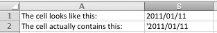
• First, some or all of the dates will be left-aligned in the cell. Date values are normally right-aligned.
• Second, you’ll notice when you click on a cell containing a date that it contains a value such as ‘2011/05/08. That apostrophe before the date is used to indicates to Excel that the value in the cell is text value, regardless of what it looks like. This feature is sometimes useful, but not in the situation we’re looking at here.

The quickest way to solve the problem, is to use the DATEVALUE function as follows:

• You have the following scenario:
  
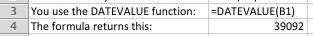
• In a cell next to the cell you want to convert, enter this formula:
  
• Note how the formula returns a number, 39092. This is the correct answer, but it has the wrong format.
  • Excel treats all dates as serial numbers. It then uses formatting to present the serial number as a date.
  • Normally, when you enter a date Excel recognises it as a date and formats it automatically. However, Excel actually stores the serial number the date represents.
  • Clearly, this didn’t happen in this example, so you’ll have to format it manually.
• There are a number of ways to format a number as a date.
  • The method is to use the Number formatting dropdown list on the Home ribbon bar. You can choose from Short Date or Long Date, or you can choose the More Number Formats option and either choose a different date format or create a custom date format. We’ll cover custom date formats in another lesson.
  • 
  • If you’re using a Mac, the the only opNumber formatting dropdown only includes Date. To choose another date format, choose Custom… 
• Once you choose a date format, the date should be presented as expected. This example shows the number in our example formatted as a date:
  
• And that’s the result we needed to get to — a text value that looked like a date but didn’t behave like one, converted into the correct date format. 

Of course, going to all of this effort doesn’t make sense when you only have a few dates that haven’t converted properly. However, if you have a large spreadsheet (e.g. with hundreds of values) the DATEVALUE function can be a real time saver.

What happens when DATEVALUE doesn’t work?

Sometimes, DATEVALUE just can’t figure out how to convert the text value into a date. Usually it’s because the text entered in the cell doesn’t look like a date. Or, it could be that the text in the cell is actually a number that you know to be a date, but which Excel doesn’t recognise as a date (or at least, doesn’t recognise it for the date we know it to be).

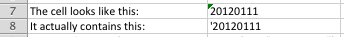
• Here’s an example of a text value that looks like a date but which just doesn’t convert with DATEVALUE:
  • 20120111
• It’s not obvious to Excel that this is a date, so DATEVALUE doesn’t know what to do with it — it will just return a #VALUE error instead.

Option One — Combine DATEVALUE with the TEXT function

However, in this example we know that this is a date. We can break it out into its constituent parts — the year is 2012, the month is January, and the day is 11. Given this, we can use the TEXT function to help us out.

Option Two — A clever and obscure use of the TEXT function

Assuming the approach shown in Option One works in your particular example, Option Two will give you a better way of getting to the same answer.

Option Three — Splitting the text into its constituent parts and recombining them into a date

The final method you can use when DATEVALUE doesn’t deliver what you want is also the most cumbersome — but potentially the most flexible. Once you know this method, there are all sorts of uses you can put it to that have nothing to do with dates. I’ve already covered it in another lesson, Extract text from a cell in Excel, but it’s worth showing you how to apply the method in this specific scenario.

• As before, we’re trying to convert this text value to a date:
  
• You can then use the LEFT, MID and RIGHT functions to extract the year, the month and the day from the text value. From there, you can use the DATE function to recombine them into something that Excel recognises as a date.
  • The LEFT function allows you to choose a specified number of characters from the left end (i.e. the beginning) of a text value.
  • The RIGHT function does the same as LEFT but starts from the right end of the text value.
  • The MID function allows you to choose a specified number of characters from a specified starting point within the cell. In fact, you can do what we need with just the MID function, but let’s look at how we might use all three.
  • The DATE function takes a Year, a Month and a Day and combines them into a date (which Excel automatically formats as a date).
• Here’s what this method looks like when applied to our problem:
  
• Let’s break it out so you can see how it works:
  • The LEFT function extracted the first four characters (the Year) from the cell B7 (i.e. the first four characters in the cell)
  • The MID function extracted two characters (the Month) from B7 starting from the 5th character from the left
  • The RIGHT function extracted two characthers (the Day) from B7 starting from the right (i.e. the last two characters in the cell)
  • The DATE function combined the Year, Month and Day into a date, and then Excel formatted it for us.
• Some points to consider with this solution:
  • You could have used the MID function in place of the LEFT and RIGHT functions had you wanted to. I leave that to you to figure out. I used all three functions in this example because the LEFT and RIGHT functions are sometimes very useful on their own, so I wanted you to see them in action.
  • If you have a value that includes a time as well as a date, you can use the TIME function to convert the time portion of the text into a valid time, and add the results together to get a valid date/time. There is an example of converting text to both a date and time in the comments below.
  • There are many, many scenarios where a formula that combines LEFT, RIGHT and MID will prove very handy. This has been just one of them.

A final word on working with Dates in Excel

Dates are always problematic, and Excel’s treatment of them can often cause confusion. One thing I have not addressed in this lesson until now is the fact that the US uses a date format that is different to most of the rest of the world. Specifically:

• The US refers to dates in the format «month, day, year»
• The rest of the world (ROW) refers to dates in the format «day, month, year»

That means that when you’re working with dates in Excel, you need to know which date format your computer is set up to use (Excel takes its lead from the computer’s date settings). Otherwise you can get some strange behaviour — and errors — showing up in Excel.

This example shows how confusion can arise.

• The date 04/05/2013 in the US refers to the 5th of April, 2013.
• In the ROW, it refers to the 4th of May, 2013.
• When sharing a spreadsheet with a colleage that uses a different date format to you, Excel will automatically switch the dates around so they appear in the correct format. But if you’re working with a system that, unbeknown to you, is using a different format, you can get into all sorts of trouble.

This example shows how things can get even worse:

• The date 04/14/2013 in the US refers to the 14th of April, 2013.
• For the ROW, typing this into Excel would generate an error since there are only 12 months in the year, not 14.

On a day to day basis, most Excel power users are used to this problem and normally see it coming. But even the best of us can have a moment of confusion when a formula we tried to write comes back with the wrong answer or an error, before we realise what the cause is, and move on. In practical terms, when using the methods shown in this lesson for converting text values into dates, be aware that how you construct your formulas may depend on the date format being used in your copy of Excel.

In this guide, we’ll learn how to change date format in Excel. Date and Time data is an integral part of any statistical document or sheet. It is important to accurately track and analyze events, sales, figures, and others.

By convention, Excel uses a general data format that may be as per your need. But in most cases, that format may need to be customized.

Changing the format of Date in a particular cell or all the cells in your Excel sheet is an easy process and doesn’t require any complex methodologies. Excel provides a wide range of formatting options based on Location and Languages which helps in better date formatting in native language and style. Also, For some Languages there is also features to select from different Calendar types.

Follow the below step-by-step tutorial to change date format in Excel quickly and easily.

Step 1. Select the range of cells containing the date

To start with, select the cell values where want to change the date format, as shown in the image below.

Step 2. Go to Number Format dropdown

• To select ‘Number Format’, go to ‘Home‘ in the option menu and look for Number Format, as shown below
• Then from the drop-down menu, select ‘More Number Formats‘ to reveal the ‘Number Format’ dialogue menu.

• Alternatively, you may directly go to Number Format, by right-clicking on the selected cell/s
• Click on ‘Number Format’.

Step 3. Choose Date

• From the Category menu on the right, choose ‘Date‘.

Now, to apply any date formatting type, select it from the right panel of the pop-up menu of Number Format. Click on ‘OK‘ to apply the formatting to the selected cell/s.

Note: You may check the date format implementation in the ‘Sample‘ at the top of the menu option

Choose the Date Type

The general option type to choose from a variety of Date Formatting options. Scroll down in this section to reveal a plethora of options for formatting, ranging from date, text (month name), year, and others.

This option can be perceived as the display menu, as the formatting options in this will keep on changing as per the selection in Locale(Location) and Calendar type.

Choose the Locale (location)

This option features the Location or Language options to help format the date accordingly. This option is probably the most used option as users require to format the date according to their or audience preference as per the native formatting style, based on language and location.

Choose any language or Location from this options menu. After selecting, all the supported date format options available for that particular locale will be available for selecting in the above Type menu.

Choose the type of calendar

This option reveals different calendar types available based on the Locale(Location) selected from the above option menu. This formatting option is only available for certain Locale and not all.

As shown in our example below, the variety of calendar types available for selection are only available for the Locale (location) selected (here, Arabia), for other locales the calendar type might be different or not at all present.

To apply selected formatting, you will need to click ‘OK‘ after selection to apply to your dates.

Conclusion

That’s It! You can now easily convert your dates to your desired format style easily.

We hope you learned and enjoyed this lesson and we’ll be back soon with another awesome Excel tutorial at QuickExcel!

Bottom Line: Use the Find & Replace feature in Excel to quickly convert text to dates.

Skill Level: Beginner

Video Tutorial

Download the Excel File

You’re welcome to use the same expense sheet that I’ve used as an example in the video. You can download it here:

Converting Text to Date Format

You might find that when you export data from online and financial programs such as QuickBooks Online, cells that are formatted as a date don’t transfer over with the same format. They may look like dates, but they their data type is actually text.

I’d like to show you a quick tip to quickly convert all of those text cells to dates.

How to Tell If Your Dates Are Actually Text

A couple of quick ways to tell if the data type for your cell is text or date include taking a look at either the number format drop-down menu or the filter drop-down menu.

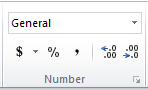
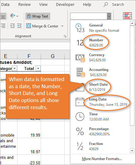
Number Format Drop-Down

If you go to the Number Format drop-down menu on the Home tab, you will see how the formatting would look for each of the categories in the drop-down. When the data is text, you can see that the Number, Short Date, and Long Date options all look the same because Excel is not recognizing the data as a date.

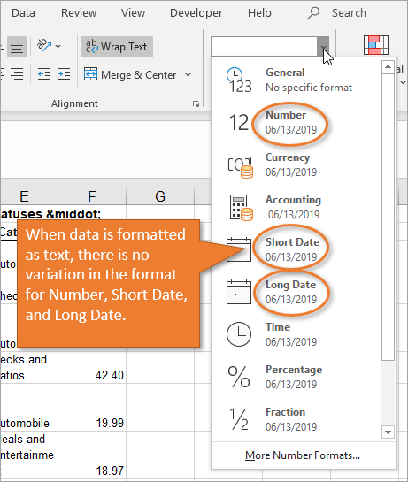
If the cells were in date format, they would look like this instead:

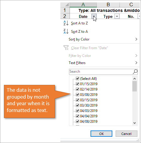
Filter Drop-Down

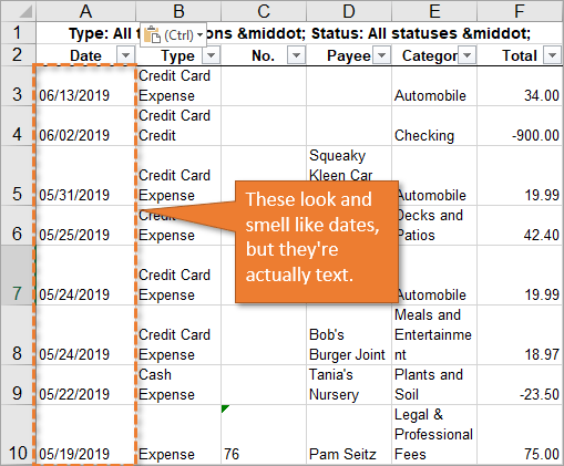
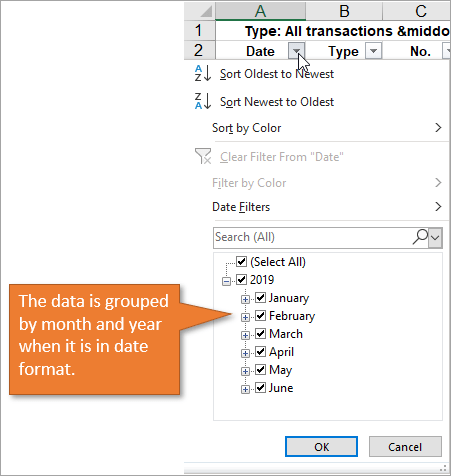
Another way to tell if a column of data is in text format is to look at the filter drop-down. If the entries aren’t being grouped by Excel into months and years, Excel is not recognizing them as dates.

When formatted as dates, you can see the month and year groupings like this:

Use Find & Replace to Evaluate Cells

A quick and easy way for Excel to evaluate these cells and to recognize them as dates is to use the Find & Replace feature. On the Home tab of the Ribbon, click on the Find & Select menu and choose Replace….

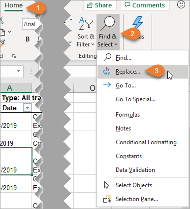
This brings up the Find and Replace window. (The keyboard shortcut to bring up this window is Ctrl + H.)

If your dates are formatted with forward slashes (/), you are going to enter a forward slash into BOTH the Find what and Replace with fields. If your dates are formatted with dashes (-), then use dashes.

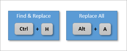
Then click Replace All. (The keyboard shortcut for Replace All is Alt + A.)

By replacing these symbols, you are essentially forcing Excel to take a look at each of the cells you’ve selected, so that it can recognize their contents as dates.

Keyboard Shortcuts

Here are the keyboard shortcuts to open the Find & Replace Window and Replace All. Alt + i is the shortcut for Find All on the Find window, which is another one I use frequently.

What If My Default Date Format is Different?

The Find and Replace technique will NOT work if your regional date format is different from the date format that the data is in.

In this example the date uses the following format: mm/dd/yyyy

I am in the U.S. and this is the same as the regional date format we use. The regional date format is set in the operating system (Windows or MacOS), NOT in Excel.

If you are in a different country and your regional date format is dd/mm/yyyy or something different, then this technique will not work.

Workarounds

There are still many ways to convert the text to dates.

You can change the regional date settings in your operating system to match the date format in the data. I wouldn’t recommend this unless you are only dealing with data from another country and constantly running into this issue.

Another option is to use Text to Columns or one of the other suggestions made in the comments section below. I will do a follow-up post on some of those solutions.

*A big thanks to Pieter, Simon, and Jonathan for pointing out this issue in the comments. We appreciate your support!

Bonus Tip

If you are exporting from an online or financial system, see if there is an option to export your data in a .CSV file. If so, it can help to avoid this problem of exporting dates as text.

Conclusion

So, if you find that your filter drop-down menu isn’t grouping by month and year, or date specific formulas are not calculating correctly, you should check your data to make sure Excel is reading it as a date data type. If not, a quick run through the Find & Replace feature should set things straight.

What other ways would you go about fixing this problem? Please leave a comment below with suggestions on other techniques you would use.

Thank you! 🙂