
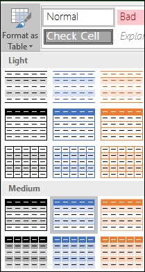
Excel provides numerous predefined table styles that you can use to quickly format a table. If the predefined table styles don’t meet your needs, you can create and apply a custom table style. Although you can delete only custom table styles, you can remove any predefined table style so that it is no longer applied to a table.

You can further adjust the table formatting by choosing Quick Styles options for table elements, such as Header and Total Rows, First and Last Columns, Banded Rows and Columns, as well as Auto Filtering.
Note: The screen shots in this article were taken in Excel 2016. If you have a different version your view might be slightly different, but unless otherwise noted, the functionality is the same.
Choose a table style
When you have a data range that is not formatted as a table, Excel will automatically convert it to a table when you select a table style. You can also change the format for an existing table by selecting a different format.
-
Select any cell within the table, or range of cells you want to format as a table.
-
On the Home tab, click Format as Table.

-
Click the table style that you want to use.
Notes:
-
Auto Preview — Excel will automatically format your data range or table with a preview of any style you select, but will only apply that style if you press Enter or click with the mouse to confirm it. You can scroll through the table formats with the mouse or your keyboard’s arrow keys.
-
When you use Format as Table, Excel automatically converts your data range to a table. If you don’t want to work with your data in a table, you can convert the table back to a regular range while keeping the table style formatting that you applied. For more information, see Convert an Excel table to a range of data.
Important:
-
Once created, custom table styles are available from the Table Styles gallery under the Custom section.
-
Custom table styles are only stored in the current workbook, and are not available in other workbooks.
Create a custom table style
-
Select any cell in the table you want to use to create a custom style.
-
On the Home tab, click Format as Table, or expand the Table Styles gallery from the Table Tools > Design tab (the Table tab on a Mac).
-
Click New Table Style, which will launch the New Table Style dialog.
-
In the Name box, type a name for the new table style.
-
In the Table Element box, do one of the following:
-
To format an element, click the element, then click Format, and then select the formatting options you want from the Font, Border or Fill tabs.
-
To remove existing formatting from an element, click the element, and then click Clear.
-
-
Under Preview, you can see how the formatting changes that you made affect the table.
-
To use the new table style as the default table style in the current workbook, select the Set as default table style for this document check box.

Delete a custom table style
-
Select any cell in the table from which you want to delete the custom table style.
-
On the Home tab, click Format as Table, or expand the Table Styles gallery from the Table Tools > Design tab (the Table tab on a Mac).
-
Under Custom, right-click the table style that you want to delete, and then click Delete on the shortcut menu.
Note: All tables in the current workbook that are using that table style will be displayed in the default table format.
-
Select any cell in the table from which you want to remove the current table style.
-
On the Home tab, click Format as Table, or expand the Table Styles gallery from the Table Tools > Design tab (the Table tab on a Mac).
-
Click Clear.
The table will be displayed in the default table format.
Note: Removing a table style does not remove the table. If you don’t want to work with your data in a table, you can convert the table to a regular range. For more information, see Convert an Excel table to a range of data.
There are several table style options that can be toggled on and off. To apply any of these options:
-
Select any cell in the table.
-
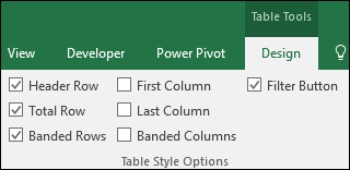
Go to Table Tools > Design, or the Table tab on a Mac, and in the Table Style Options group, check or uncheck any of the following:
-
Header Row — Apply or remove formatting from the first row in the table.
-
Total Row — Quickly add SUBTOTAL functions like SUM, AVERAGE, COUNT, MIN/MAX to your table from a drop-down selection. SUBTOTAL functions allow you to include or ignore hidden rows in calculations.
-
First Column — Apply or remove formatting from the first column in the table.
-
Last Column — Apply or remove formatting from the last column in the table.
-
Banded Rows — Display odd and even rows with alternating shading for ease of reading.
-
Banded Columns — Display odd and even columns with alternating shading for ease of reading.
-
Filter Button — Toggle AutoFilter on and off.
-
In Excel for the web, you can apply table style options to format the table elements.
Choose table style options to format the table elements
There are several table style options that can be toggled on and off. To apply any of these options:
-
Select any cell in the table.
-
On the Table Design tab, under Style Options, check or uncheck any of the following:
-
Header Row — Apply or remove formatting from the first row in the table.
-
Total Row — Quickly add SUBTOTAL functions like SUM, AVERAGE, COUNT, MIN/MAX to your table from a drop-down selection. SUBTOTAL functions allow you to include or ignore hidden rows in calculations.
-
Banded Rows — Display odd and even rows with alternating shading for ease of reading.
-
First Column — Apply or remove formatting from the first column in the table.
-
Last Column — Apply or remove formatting from the last column in the table.
-
Banded Columns — Display odd and even columns with alternating shading for ease of reading.
-
Filter Button — Toggle AutoFilter on and off.
-
Содержание
- Create and format tables
- Try it!
- Ways to format a worksheet
- How to control and understand settings in the Format Cells dialog box in Excel
- Summary
- More Information
- Number Tab
- Auto Number Formatting
- Built-in Number Formats
- Custom Number Formats
Create and format tables
Create and format a table to visually group and analyze data.
Note: Excel tables shouldn’t be confused with the data tables that are part of a suite of What-If Analysis commands ( Forecast, on the Data tab). See Introduction to What-If Analysis for more information.

Try it!
Select a cell within your data.
Select Home > Format as Table.
Choose a style for your table.
In the Create Table dialog box, set your cell range.
Mark if your table has headers.
Insert a table in your spreadsheet. See Overview of Excel tables for more information.
Select a cell within your data.
Select Home > Format as Table.
Choose a style for your table.
In the Create Table dialog box, set your cell range.
Mark if your table has headers.
To add a blank table, select the cells you want included in the table and click Insert > Table.
To format existing data as a table by using the default table style, do this:
Select the cells containing the data.
Click Home > Table > Format as Table.
If you don’t check the My table has headers box, Excel for the web adds headers with default names like Column1 and Column2 above the data. To rename a default header, double-click it and type a new name.
Note: You can’t change the default table formatting in Excel for the web.
Источник
Ways to format a worksheet
In Excel, formatting worksheet (or sheet) data is easier than ever. You can use several fast and simple ways to create professional-looking worksheets that display your data effectively. For example, you can use document themes for a uniform look throughout all of your Excel spreadsheets, styles to apply predefined formats, and other manual formatting features to highlight important data.
A document theme is a predefined set of colors, fonts, and effects (such as line styles and fill effects) that will be available when you format your worksheet data or other items, such as tables, PivotTables, or charts. For a uniform and professional look, a document theme can be applied to all of your Excel workbooks and other Office release documents.
Your company may provide a corporate document theme that you can use, or you can choose from a variety of predefined document themes that are available in Excel. If needed, you can also create your own document theme by changing any or all of the theme colors, fonts, or effects that a document theme is based on.
Before you format the data on your worksheet, you may want to apply the document theme that you want to use, so that the formatting that you apply to your worksheet data can use the colors, fonts, and effects that are determined by that document theme.
For information on how to work with document themes, see Apply or customize a document theme.
A style is a predefined, often theme-based format that you can apply to change the look of data, tables, charts, PivotTables, shapes, or diagrams. If predefined styles don’t meet your needs, you can customize a style. For charts, you can customize a chart style and save it as a chart template that you can use again.
Depending on the data that you want to format, you can use the following styles in Excel:
Cell styles To apply several formats in one step, and to ensure that cells have consistent formatting, you can use a cell style. A cell style is a defined set of formatting characteristics, such as fonts and font sizes, number formats, cell borders, and cell shading. To prevent anyone from making changes to specific cells, you can also use a cell style that locks cells.
Excel has several predefined cell styles that you can apply. If needed, you can modify a predefined cell style to create a custom cell style.
Some cell styles are based on the document theme that is applied to the entire workbook. When you switch to another document theme, these cell styles are updated to match the new document theme.
For information on how to work with cell styles, see Apply, create, or remove a cell style.
Table styles To quickly add designer-quality, professional formatting to an Excel table, you can apply a predefined or custom table style. When you choose one of the predefined alternate-row styles, Excel maintains the alternating row pattern when you filter, hide, or rearrange rows.
For information on how to work with table styles, see Format an Excel table.
PivotTable styles To format a PivotTable, you can quickly apply a predefined or custom PivotTable style. Just like with Excel tables, you can choose a predefined alternate-row style that retains the alternate row pattern when you filter, hide, or rearrange rows.
For information on how to work with PivotTable styles, see Design the layout and format of a PivotTable report.
Chart styles You apply a predefined style to your chart. Excel provides a variety of useful predefined chart styles that you can choose from, and you can customize a style further if needed by manually changing the style of individual chart elements. You cannot save a custom chart style, but you can save the entire chart as a chart template that you can use to create a similar chart.
For information on how to work with chart styles, see Change the layout or style of a chart.
To make specific data (such as text or numbers) stand out, you can format the data manually. Manual formatting is not based on the document theme of your workbook unless you choose a theme font or use theme colors — manual formatting stays the same when you change the document theme. You can manually format all of the data in a cell or range at the same time, but you can also use this method to format individual characters.
For information on how to format data manually, see Format text in cells.
To distinguish between different types of information on a worksheet and to make a worksheet easier to scan, you can add borders around cells or ranges. For enhanced visibility and to draw attention to specific data, you can also shade the cells with a solid background color or a specific color pattern.
If you want to add a colorful background to all of your worksheet data, you can also use a picture as a sheet background. However, a sheet background cannot be printed — a background only enhances the onscreen display of your worksheet.
For information on how to use borders and colors, see:
For the optimal display of the data on your worksheet, you may want to reposition the text within a cell. You can change the alignment of the cell contents, use indentation for better spacing, or display the data at a different angle by rotating it.
Rotating data is especially useful when column headings are wider than the data in the column. Instead of creating unnecessarily wide columns or abbreviated labels, you can rotate the column heading text.
For information on how to change the alignment or orientation of data, see Reposition the data in a cell.
If you have already formatted some cells on a worksheet the way that you want, there are several ways to copy just those formats to other cells or ranges.
Home > Paste > Paste Special > Paste Formatting.
Home > Format Painter  .
.
Right click command
Point your mouse at the edge of selected cells until the pointer changes to a crosshair.
Right click and hold, drag the selection to a range, and then release.
Select Copy Here as Formats Only.
Tip If you’re using a single-button mouse or trackpad on a Mac, use Control+Click instead of right click.
Data range formats are automatically extended to additional rows when you enter rows at the end of a data range that you have already formatted, and the formats appear in at least three of five preceding rows. The option to extend data range formats and formulas is on by default, but you can turn it on or off by:
Newer versions Selecting File > Options > Advanced > Extend date range and formulas (under Editing options).
Excel 2007 Selecting Microsoft Office Button  > Excel Options > Advanced > Extend date range and formulas (under Editing options)).
Источник
How to control and understand settings in the Format Cells dialog box in Excel
Summary
Microsoft Excel lets you change many of the ways it displays data in a cell. For example, you can specify the number of digits to the right of a decimal point, or you can add a pattern and border to the cell. You can access and modify the majority of these settings in the Format Cells dialog box (on the Format menu, click Cells).
The «More Information» section of this article provides information about each of the settings available in the Format Cells dialog box and how each of these settings can affect the way your data is presented.
More Information
There are six tabs in the Format Cells dialog box: Number, Alignment, Font, Border, Patterns, and Protection. The following sections describe the settings available in each tab.
Number Tab
Auto Number Formatting
By default, all worksheet cells are formatted with the General number format. With the General format, anything you type into the cell is usually left as-is. For example, if you type 36526 into a cell and then press ENTER, the cell contents are displayed as 36526. This is because the cell remains in the General number format. However, if you first format the cell as a date (for example, d/d/yyyy) and then type the number 36526, the cell displays 1/1/2000.
There are also other situations where Excel leaves the number format as General, but the cell contents are not displayed exactly as they were typed. For example, if you have a narrow column and you type a long string of digits like 123456789, the cell might instead display something like 1.2E+08. If you check the number format in this situation, it remains as General.
Finally, there are scenarios where Excel may automatically change the number format from General to something else, based on the characters that you typed into the cell. This feature saves you from having to manually make the easily recognized number format changes. The following table outlines a few examples where this can occur:
| If you type | Excel automatically assigns this number format |
|---|---|
| 1.0 | General |
| 1.123 | General |
| 1.1% | 0.00% |
| 1.1E+2 | 0.00E+00 |
| 1 1/2 | # ?/? |
| $1.11 | Currency, 2 decimal places |
| 1/1/01 | Date |
| 1:10 | Time |
Generally speaking, Excel applies automatic number formatting whenever you type the following types of data into a cell:
Built-in Number Formats
Excel has a large array of built-in number formats from which you can choose. To use one of these formats, click any one of the categories below General and then select the option that you want for that format. When you select a format from the list, Excel automatically displays an example of the output in the Sample box on the Number tab. For example, if you type 1.23 in the cell and you select Number in the category list, with three decimal places, the number 1.230 is displayed in the cell.
These built-in number formats actually use a predefined combination of the symbols listed below in the «Custom Number Formats» section. However, the underlying custom number format is transparent to you.
The following table lists all of the available built-in number formats:
| Number format | Notes |
|---|---|
| Number | Options include: the number of decimal places, whether or not the thousands separator is used, and the format to be used for negative numbers. |
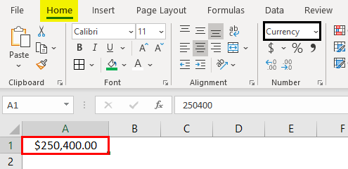
| Currency | Options include: the number of decimal places, the symbol used for the currency, and the format to be used for negative numbers. This format is used for general monetary values. |
| Accounting | Options include: the number of decimal places, and the symbol used for the currency. This format lines up the currency symbols and decimal points in a column of data. |
| Date | Select the style of the date from the Type list box. |
| Time | Select the style of the time from the Type list box. |
| Percentage | Multiplies the existing cell value by 100 and displays the result with a percent symbol. If you format the cell first and then type the number, only numbers between 0 and 1 are multiplied by 100. The only option is the number of decimal places. |
| Fraction | Select the style of the fraction from the Type list box. If you do not format the cell as a fraction before typing the value, you may have to type a zero or space before the fractional part. For example, if the cell is formatted as General and you type 1/4 in the cell, Excel treats this as a date. To type it as a fraction, type 0 1/4 in the cell. |
| Scientific | The only option is the number of decimal places. |
| Text | Cells formatted as text will treat anything typed into the cell as text, including numbers. |
| Special | Select one of the following from the Type box: Zip Code, Zip Code + 4, Phone Number, and Social Security Number. |
Custom Number Formats
If one of the built-in number formats does not display the data in the format that you require, you can create your own custom number format. You can create these custom number formats by modifying the built-in formats or by combining the formatting symbols into your own combination.
Before you create your own custom number format, you need to be aware of a few simple rules governing the syntax for number formats:
Each format that you create can have up to three sections for numbers and a fourth section for text.
The first section is the format for positive numbers, the second for negative numbers, and the third for zero values.
These sections are separated by semicolons.
If you have only one section, all numbers (positive, negative, and zero) are formatted with that format.
You can prevent any of the number types (positive, negative, zero) from being displayed by not typing symbols in the corresponding section. For example, the following number format prevents any negative or zero values from being displayed:
To set the color for any section in the custom format, type the name of the color in brackets in the section. For example, the following number format formats positive numbers blue and negative numbers red:
Instead of the default positive, negative and zero sections in the format, you can specify custom criteria that must be met for each section. The conditional statements that you specify must be contained within brackets. For example, the following number format formats all numbers greater than 100 as green, all numbers less than or equal to -100 as yellow, and all other numbers as cyan:
Источник
In this lesson you can learn everything about formatting in Excel.
Formatting can be done in Excel in two ways:
- Using one of the prepared style (tables, charts, etc.) or
- Formatting separated elements.
Using the prepared style is comfortable for novice users who use the standard tables or charts. Persons who wish to have full control over the appearance of a worksheet, or documents prepared by them do not fit within the imposed format, choose self-formatting. Using styles is discussed at the end of this lesson.
Method 1 Formatting step by step
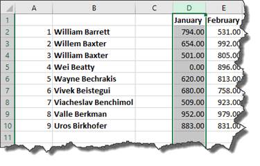
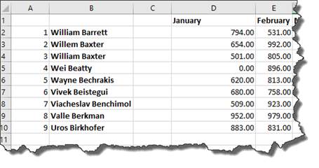
Suppose we were asked to prepare a table of data in the system as below. We managed to collect relevant data and paste them into the table. The following table, however, has many drawbacks.

Change width of columns and rows
We’ll start with the fact that all data and descriptions of the categories are shown. At this time, the data in the cells ‘I23’ and ‘I32’ do not fit in the current column width and have been replaced by Excel on the symbols # # #.Similarly.
The descriptions in cells B10 and B32 are also not shown in its entirety. To expand a column will be most convenient to double-click on the dash between the columns. You can also click and drag the left button to expand the column width to the desired size.

For columns of equal width, select all of which are to be aligned and drag the width of any of them to the desired size.

Insert / delete rows
The next step is the removal of three rows at the beginning of the table. To do this, select the first three rows of the worksheet, select the rows by clicking on the symbol ‘1 ‘and holding the left mouse button pressed drag the selection to three-line, where he let go hold down the left key. Once selected, click on one of the signs of rows (1.2 or 3) and with the right mouse button menu that will select the Delete option.

Will be deleted as many items as you previously selected. In the same way, you can insert rows or columns (the command ‘Insert’). Let’s insert now one line before the table.

Borders
When you insert a row at the beginning of the worksheet, you activate the entire table and clicked on the icon bar arrow next to ‘Borders’ Proposes to select ‘All edges’ (marked in the figure below) for the entire table. Then ‘thick edge of the field’ (the two commands below) to make a bold border.

Now you can select only the cells of the column headers and select them again in bold borders. You will do the same for the row. You do not need every time to develop menu Borders, the last of the commands will be executed when you click the selected icons in the figure below.

Border icons provide basic and most frequently used border, but you wanted to take advantage of dual or diagonal lines dividing cells should click with right mouse button on a selected cell, or the previously selected area and a menu that shows up, select ‘Format Cells…’.

Window appears and ‘Format Cells’ on the ‘border’ you have all the formatting options that Excel offers. First, choose what format the line we are interested in the ‘Style’ and then click on the right side to indicate where the line is to be found, choose a diagonal line marked red square.

Merge cells
Another operation will merge cells. In cells B2 and B3 are diagonal lines that do not look good.

Select the cells you want to merge and click the icon for ‘Merge and center’.


Result merging is presented below. Also merge the cells that contain the repeated column headers.

A message appears that symbols of 2 cells 1Q with a gray background in the picture above will be deleted. Click OK.

After the cells merged, I2 and I3, we find that we would prefer to headline 1HY (first half of the year) was displayed at half height of the new merged cell. Click the right mouse button and choose the command ‘Format Cells …’.

In the ‘Format Cells’ on the ‘Alignment’ choose ‘agent’ in the menu ‘Vertical’.

Change cell background color
Change the background color of a cell or cell area, is to select the cell / area, click on the arrow next to ‘fill color’ (shown in the figure below) and select the desired color.

If we again color the cells of the same color, we need not choose it again, he was remembered, and simply click on the icon ‘fill color’.

Format Painter
If you have some kind of format the cell, column or row and want you to another cell or area have the same format, instead of repeating all the operations from scratch, you better use the Format Painter. Format the line 21, as shown below. For bold, click the icon for B. The next step will be to change the color of cells, so that the aggregated data for the categories stand out.

Just want to format several other rows. Of course, not every time we repeat the same steps, but we will use the ‘Format Painter’. Select the area of ‘pattern’, i.e. the line of 21st Click the Format Painter icon (paintbrush).

Click in cell B25 and the entire row of the table takes the appropriate format.

You can copy formatting from one cell immediately adjacent to a larger number of cells and copy the formatting of a larger area to the area. It is not possible to copy the format once again after the first copy, Excel, ‘forget’ model after its first use and the operation must be repeated. Another way to format a number of areas so it is the simultaneous selection before formatting. To select multiple areas at once is enough while selecting with the mouse hold down the Ctrl button.
Grid lines
Reports and tables usually look better if you disable the grid lines. To enable or disable Grid lines tab to select the ‘Page Layout’, ‘Gridlines’, ‘View’.

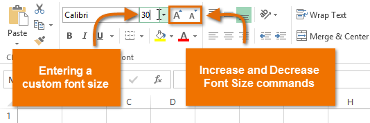
Change font size
To change the font in a cell or cell area it is easiest to select an area for which you want to do it, then select the correct size from the drop-down box located in the icons (shown below). I recommend using the icons next to the first of which enlarges the font and the other decreases.

Hide / unhide rows and columns
Hiding rows or columns is to select them. To select all rows at once and all the columns simply click the left mouse button on the rectangle marked in the figure below a red circle.

To then discover all the rows, click the right mouse button on any determination of the line (below the red circle) and the menu that will select, Discover ‘, do the same for columns to give us the assurance that all cells in the spreadsheet are visible.

The data in hidden cells remain unchanged and are still employed by the formula. NOTE: The charts in Excel do not use the data in hidden cells.
Avoiding the destruction of formatting
The basic principle should be to format the cell deposition at the end of our work, once we sure that the system will be our report. If we do this earlier, pasting, copying and other operations, they can spoil our format and we have to do it again. Often, however, after the formatting changes are inevitable.
Style
Excel developers have prepared several formats, which can be used in preparing documents in Excel. Their biggest advantage is that inexperienced users can quickly get Excel sheet professional. Styles work correctly only for simple tables or other objects.
Method 2 Formatting as a Table
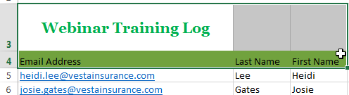
On the worksheet ‘Format 2’ is a table of data. It contains only one row of column headers and does not have catfished, so it can be formatted as a table. Set the active cell in any table cell and from your ‘Home’ to choose ‘Format as Table’, then choose the color model that suits us.

A window will appear, in which we are asked to confirm whether the area of the table was properly recognized. Click OK.

The table is formatted according to the selected model. If it does not suit us, that header cells contain symbols of the filter can be disabled by selecting ‘Sort & Filter’ and then click ‘Filter’.

When you click the right mouse button on the table, we can add a row sum, as is shown below.

Sum which will be introduced only for June, copy to the other months.

Exercise can be considered completed.

This way, you can not format the table of Example 1 because it contains two rows of column headers. Example 3 There is a column chart. When you select it (by clicking on it with the left mouse button), command tabs appear: ‘Design’, ‘system’ and ‘Format’. On the ‘Design’ styles will find a chart, click on the arrow marked below the red square to view all available styles.

Choose the style that suits us and click on it.

After changing chart style, even change the font style of his title. Select the title by clicking on it and the cards ‘Format’ select one of the Word Art styles.

Formatting Excel spreadsheets to be sure the look was tailored to the tasks to be satisfied by a given sheet. A common mistake of beginners is the use of sophisticated style to impress the recipient, but it does only feel the lack of professional approach.
Further reading:
Status Bar
Keyboard shortcuts
Display Cells Containing Formulas
The maximum width for a column is 255 if the default font and font size is used. The minimum width is zero, of course. If a column width is zero, the column will be hidden.
To set a column to a specific width, select the column that you want to format.
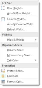
Next, go to the Cells group under the Home tab. Click the Format dropdown menu.
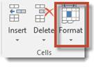
Pictured below is the dropdown menu.

Select Column Width.
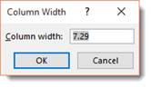
Type in the width of the column, keeping in mind that it reflects the number of characters that can be displayed.
Change the Width of the Column to Fit the Contents
Maybe you just want to make sure that the columns are wide enough to display all the contents, but you don’t want to take the time to count characters. Perhaps you aren’t even sure how many characters there will be, but want to make sure the column will be wide enough anyway.
To do this, go back to the Format dropdown menu. This time select AutoFit Column Width.
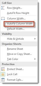
The width of all the cells in a selected column will now be determined by the cell with the most characters.
Match the Column Width to Another Column’s Width
You can also match the width of one column to the width of another column. To do this, select the column whose width you want to match.

Copy the column by right clicking and selecting copy.
Next, select the column whose width you want to change. Right click within a cell in that column and select Paste Special.

Put a check by Column Widths, then click OK.
As you can see, the column width of column D has been expanded to match the column width in column B.
Change the Default Width for All Columns in a Worksheet or Workbook
To change a default column width for a worksheet, click the worksheet tab to make the worksheet active. To change it for the entire workbook, click a worksheet tab, then right click, and select Select All Sheets.
Now, go back to the Home tab and click the Format dropdown arrow again.
Select Default Width.
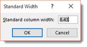
In the Standard Width box, type the new measurement.
Change the Width of Columns by Moving the Mouse
To change the width of one column using your mouse, drag the right side of the column to the right until you reach the desired width. To do so, move your mouse to the line separating two columns until you see horizontal arrows appear.
To change the width of multiple columns, select the columns that you want to change, then drag the right side of one column to its desired width.
To change the width of all the columns in a worksheet, select the entire worksheet by clicking the box to the left of column A and above row 1, then dragging the boundary of any column.
Changing Rows to a Specific Height
You follow the exact same steps to change row height as you did for columns.
To change a row to a specific height, select the row(s) that you want to change.
Go to the Home tab and click the dropdown arrow below Format.
Select Row Height.

Row height is measured in points. In the snapshot above, the row height is set at 15 points. This is the same size as font size 15.
Enter the row height, then click OK.
Change Row Height to Fit Contents
Just as you changed the width of a column to fit the contents of the widest cell in a column, you can also change the height of a row to match the height of the tallest cell.
To do this, select the rows(s) that you want to change.
Select AutoFit Row Height from the Format dropdown menu on the Ribbon.
Change a Row Height by Dragging the Mouse
You can also change the height of a row(s) by simply dragging the mouse.
To do this, select the row(s) whose height you want to change.
Next, drag the boundary below a row to adjust its height. To adjust the height of multiple rows, drag the boundary of one of them.
Definition of Format Cells
A format in excel can be defined as the change of appearance of the data in the cell the way it is, without changing the actual data or numbers in the cells. That means the data in the cell remains the same, but we will change the way it looks.
Different Formats in Excel
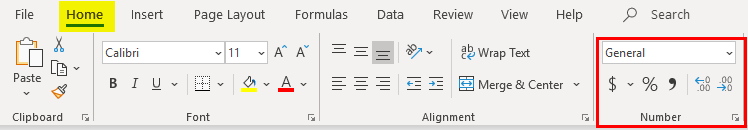
We have multiple formats in Excel to use. To see the available formats in excel, click on the “Home” menu on the top left corner.
General Format
In General format, there is no specific format; whatever you input, it will appear in the same way; it may be a number or text or symbol. After clicking on the HOME menu, go to the “NUMBER” segment, where you can find a drop of formats.
Click on the drop-down where you see the “General” option.
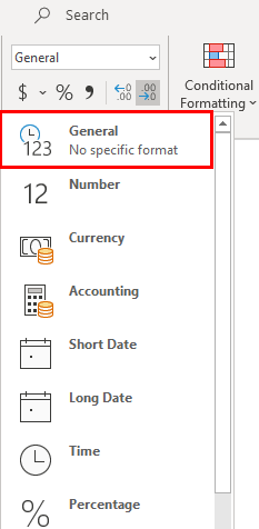
We will discuss each of these formats one by one with related examples.
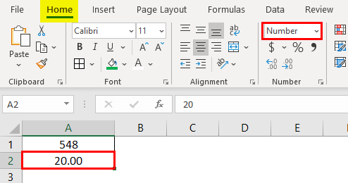
1. Number Format
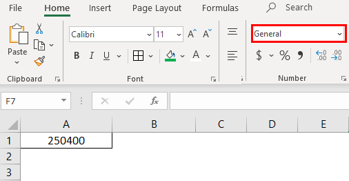
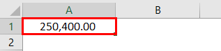
This format converts the data to a number format. When we input the data initially, it will be in General format; after converting to Number format only, it will appear as number format. Observe the below screenshot for the number in General format.
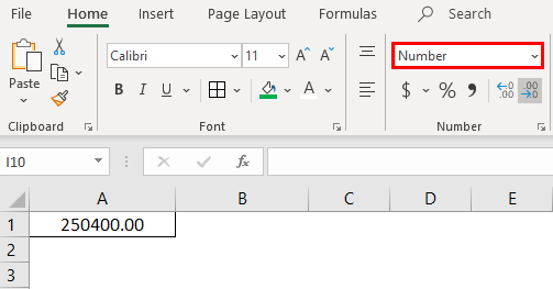
Now choose the format “Number” from the drop-down list and see how the appearance of cell A1 changes.
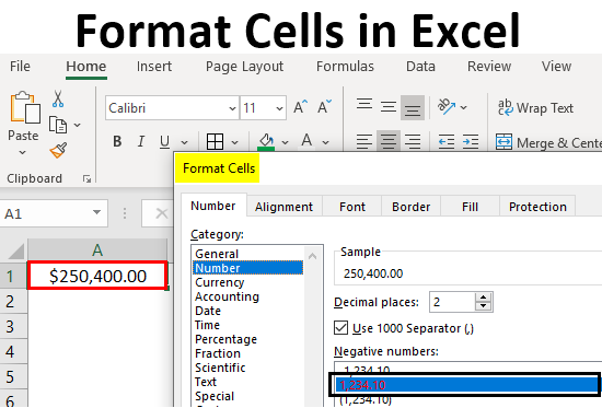
That is a difference between the General and Number format. If you want further customizations to your number format, select the cell that you want to do customization and right-click the below menu will come.
Choose the “Format Cells“ option then you will get the below window.
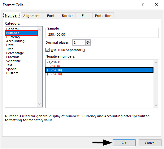
Choose “Number” under the “Category” option then you will get the customizations for the Number format. Choose the number of decimals you want to display. Tick the checkbox “Use 1000 separator” for separation of 1000’s with a comma (,).
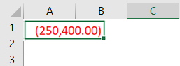
Choose the negative number format whether you want to display with a negative symbol, brackets, red colour, nd red col, etc.
2. Currency Format
Currency format helps to convert the data to a currency format. We have an option to choose the type of currency as per our requirement. Select the cell which you want to convert to Currency format and choose the “Currency” option from the drop-down.
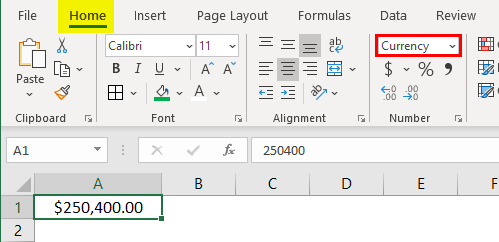
Currently, it is in Dollar currency. We can change by clicking on the drop-down of “$” and choose your required currency.
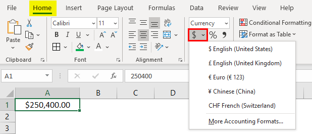
In the drop-down, we have few currencies; if you want the other currencies, click on the option “More Accounting formats”, which will display a pop-up menu as below.
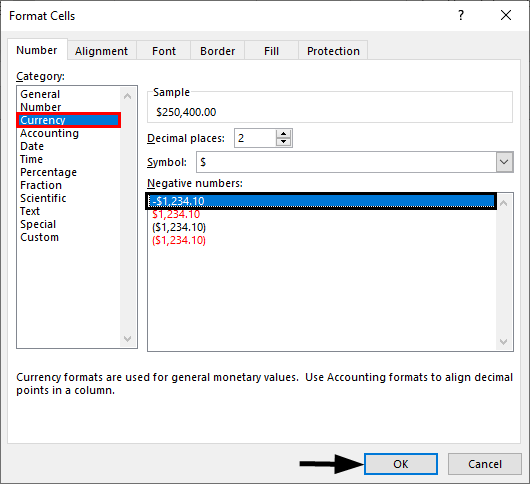
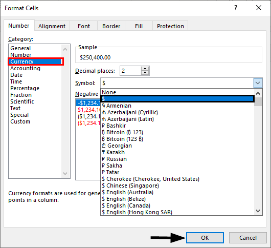
Click on the drop-down “Symbol” and choose the required currency format.
3. Accounting Format
As you all know, accounting numbers are all related to money; hence whenever we convert any number to accounting format, it will add a currency symbol to that. The difference between currency and accounting is currency symbol alignment. Below are the screenshots for reference.
4. Accounting Alignment
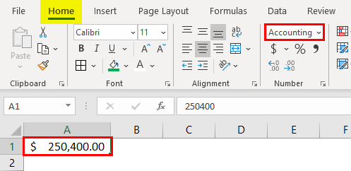
5. Currency Alignment
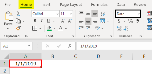
6. Short Date Format
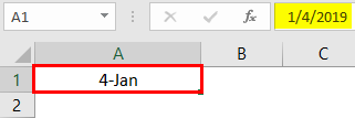
A date can represent in a short format and long format. When you want to represent your date in a short format, use the short date format. E.g., 1/1/2019.
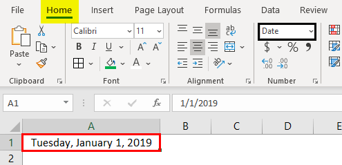
7. Long Date Format
The long date is used to represent our date in an expandable format like the below screenshot.
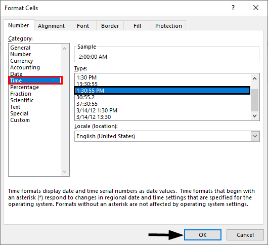
We see the short date format and long date format have multiple formats to represent our dates. Right-click and select “Format Cells” as to how we did before for “numbers”, then we will get the window to select the required formats.
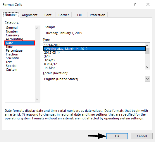
You can choose the location from the “Locale” drop-down menu.
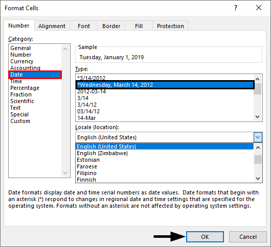
Choose the date format under the “Type” menu.
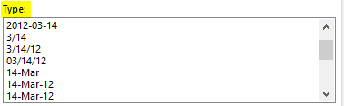
We can represent our date in any of the formats from the available formats.
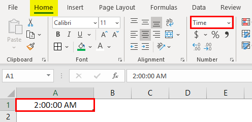
8. Time Format
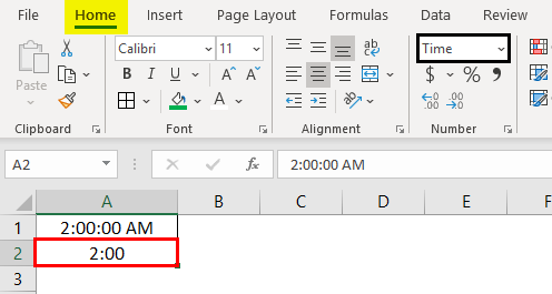
This format is used to represent the time. If you input time without converting the cell into time format, it will show normally, but if you convert the cell into time format and input, it will clearly represent the time. Find the below screenshot for the differences.
If you still want to change the time format, then change in the format cells menu as shown below.
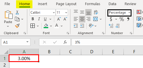
9. Percentage Format
Suppose you want to represent the number percentage use this format. Input any number in the cell and select that cell and choose the percentage format then the number will convert into a percentage.
10. Fraction Format
When we input the fraction numbers like 1/5, we should convert the cells into Fraction format. If we input the same 1/5 in a normal cell, it will show as a date.
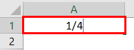

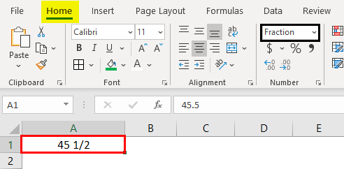
This is how the fraction format works.
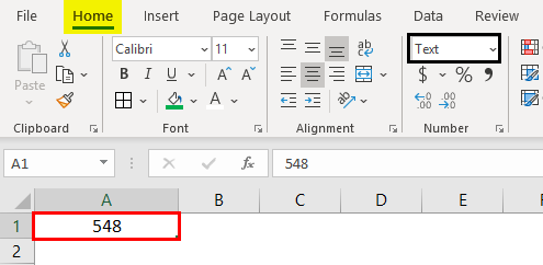
11. Text Format
When you input the number and convert it to text format, the number will align to the left side. It will consider as text as only, not the number.
12. Scientific Format
When you input a number 10000 (Ten thousand) and convert it into a scientific format, it will display as 1E+04, here E means exponent and 04 represents the number of zeros. If we input the number 0.0003, it will display as 3E-04. Try different numbers in excel format and check you will get a better idea to understand this better.
13. Other Formats
Apart from the explained formats, we have other formats like Alignment, Font, Border, Fill, and Protection.
Most of them are self-explanatory; hence I am leaving and explaining protection alone. When you want to lock any cells in the spreadsheet, use this option. But this lock will enable only when you protect the sheet.
You can hide and lock the cells on the same screen; Excel has provided instructions on when it will affect.
Things to Remember About Format Cells in Excel
- One can apply formats by right-clicking and selecting the format cells or from the drop-down as explained initially. The impact of them is the same; however, you will have multiple options when you right-click.
- When you want to apply a format to another cell, use format painter, select the cell, click on formatted painters, and choose the cell you want to apply.
- Use the option “Custom” when you want to create your own formats as per requirement.
Recommended Articles
This is a guide to Format Cells in Excel. Here we discuss how to format cells in excel along with practical examples and a downloadable excel template. You can also go through our other suggested articles to learn more–
- Excel Conditional Formatting for Dates
- Auto Format in Excel
- Formatting Text in Excel
- Excel Format Phone Numbers
If you are wondering how to format cells in excel, you have came to the right place. Small formatting adjustments can make all the difference to a Microsoft Excel workbook. A small pop of color here, a change of font there, and suddenly, your workbook is no longer just a sea of rows and columns, but an organized, presentable table of data. Knowing how to format cells in excel will help you in your data organization and preparation!
Below, we take a closer look at how to format cells in Excel tables using the six tabs found in the Format Cells dialog box, followed by some Excel format shortcuts.
What Does it Mean to Format Cells in Excel?
Microsoft Excel offers several controls that allow users to change how their data is displayed. And there’s good reason to do so—formatting cells in excel can draw attention to important data or more accurately display the contents at hand (for example, adding $ to cells that contain values pertaining to prices or configuring cells that represent dates to a standard display of xx/xx/xxxx).
Formatting cells in excel is an optional step following data preparation, or all of the data cleansing, enriching, structuring, and standardizing that is required in order to prepare data for analysis.
New data rarely arrives without its own unique set of challenges; it’s up to analysts to comb through their data and ensure that it is prepared to fit the specific needs of their analytic project. This could include splitting columns, removing rows with missing data, or standardizing against a certain name (e.g. “CA” or “Calif.” becomes “California”).
Once completed, Excel formatting adds the finishing touches so that data is both accurately prepared and presented.
What Are the Six Tabs in the Format Cells Dialog Box?
The six tabs in the Format Cells dialog box include: Number, Alignment, Font, Border, Patterns, and Protection.
Number Tab
The Number tab allows you to format the way that your numbers will be displayed. You can choose from options such as percentages, dates, currency, times, etc.
- Start by selecting the cells you want to modify.
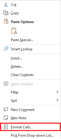
- On the Home tab, select Format > Format Cells, which will open the Format Cells dialog box.
- The first tab listed is the Number tab. The Category list in the Number tab allows you to select the format you want to use, such as Date, Time, Percentage, Currency, etc. You will also have the option to further customize your selection. For example, you could select a specific way that you’d like to represent negative currency values (see image below).

Source: Microsoft Support
Alignment Tab
Automatically, Excel formats any text to the bottom-left of a cell and numbers to the to the bottom-right. The Alignment tab within the Format Cells dialog box allows you to customize the way that you’d like your values to be aligned, both Vertically or Horizontally.
Should you require a more dramatic text alignment, the Degrees field allows text to be oriented 90 degrees in either direction up or down.
Text Control allows you to control the way Excel formats information in a cell. There are three types of text control: wrapped text, shrink to fit, and merge cells.
And finally, Text Direction switches the direction of the worksheet—in other words, column A could start from the upper right side instead of the upper left.
- To make any of these modifications, first select the text that you’d like to modify.
- On the Home tab, select Format > Format Cells, which will open the Format Cells dialog box.
- Click on the Alignment tab. From there, you will see Text Alignment (Horizontal; Vertical), Text Control (Wrap text, Shrink to fit, Merge cells) and Text Direction (Context; Left-to-Right; Right-to-Left).

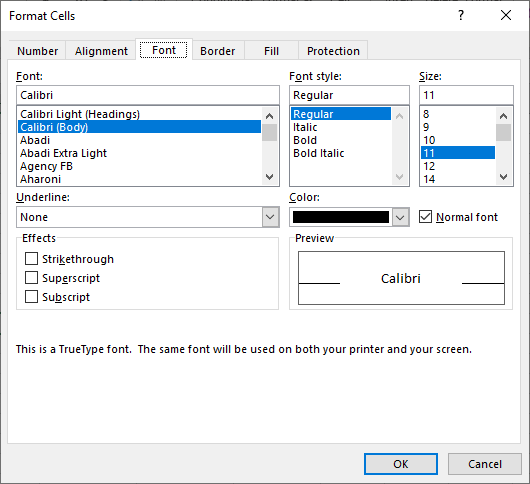
Font
Quick Font changes can be made directly from the Home tab, but for mass changes, it’s more efficient to use the Format Cells dialog box. From there, it’s easy to change typeface, point size, font size, bold, italicize, underlining, and color across an entire selection of cells.
- To make any of these modifications, first select the text that you’d like to modify.
- On the Home tab, select Format > Format Cells, which will open the Format Cells dialog box.
- Clicking on the Font tab will prompt the possible selections, as well as a preview of your changes.

Border
Excel allows you to construct borders around a single cell or a range of cells. You can determine where the lines will be drawn (for example, only the top of the cell or on all horizontal sides) and adjust their thickness, color, and line style.
- To make any of these modifications, first select the text that you’d like to modify.
- On the Home tab, select Format > Format Cells, which will open the Format Cells dialog box.
- Clicking on the Border tab will prompt the possible selections. If you want to remove a specific border, click the button for that border a second time.If you want to change the line color or style, click the style or color that you want, and then click the button for the border again.

Fill
The Fill tab in the Format Cells dialog box allows users to set the background color of all selected cells, which may include applying two-color patterns or shading from the Patterns option. Here’s how to shade cells with Patterns:
- Start by selecting the text that you’d like to modify.
- On the Home tab, select Format > Format Cells, which will open the Format Cells dialog box.
- Click on the Fill tab, then select the Pattern Style you’d like to set as the background to your cells. As an optional addition, you may also choose to set a Pattern Color to accompany your Pattern Style.
- At any time, you can return to the default state of your selected cells by choosing No Color at the top of color selection.

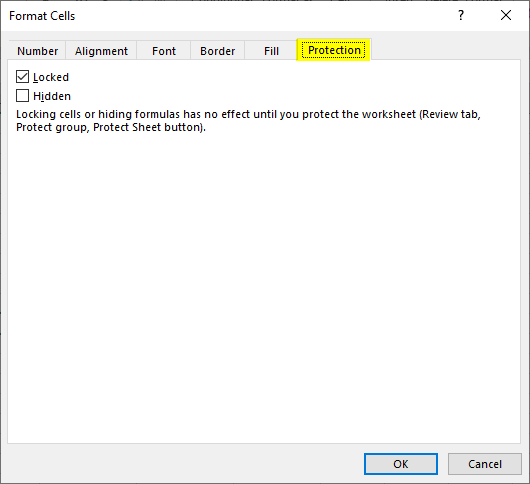
Protection
The Protection tab does not apply unless you have already protected your worksheet. To do so, click on Protection in the Tools menu, select Protect Sheet, and then select the Contents check box(es) to determine how, exactly, the worksheet will be protected.
When the Locked option is selected, you are prohibited from doing the following:
- Changing the cell data or formulas.
- Typing data in an empty cell.
- Moving the cell.
- Resizing the cell.
- Deleting the cell or its contents.
When the Hidden option is selected, that means that all formulas used to calculate values will no longer be viewable in the formula bar (however, you can still see the end result of that formula).

Recycling Excel File Formats
After you’ve formatted your Excel worksheet exactly how you want it using the six primary Excel file formats, odds are, you don’t want to keep repeating that work. Here are some of the ways that users can recycle their Excel formatting process.
Copying Styles Between Workbooks
With each new worksheet, there’s a way to copy over previous Excel file formats from an original worksheet.
- First, open the workbook with your original Excel formatting and the new workbook.
- From the original workbook, click Cell Styles in the Styles group on the Home tab.
- Choose Merge Styles at the bottom of the gallery.
- In the resulting dialog, select the open workbook that contains the styles you want to copy.
- Click OK twice.
Copy Over Formats
Sometimes you just want to copy over formatting from one column to another (without the values). In that scenario, it’s easy to copy over formatting only.
- First, start by selecting the destination cell or range of cells.
- Then, right-click the border of the cell with your preferred formatting and drag it to the target cell or range of cells.
- When you release the mouse, Excel will display a submenu where you can select “Copy Here,” “Copy Here as Values Only” or “Copy Here as Formats Only.” In this case, you’d want to select the third option, leaving the cells blank but prepped with the correct formatting.
Use Paste to Copy Formatting
In a similar vein, you can use the Paste function to copy over formatting from one column to another.
- You’ll start by selecting and copying [Ctrl]+C your original cell or range of cells.
- Then, click anywhere instead your destination cell or range of cells. Press [Ctrl]+[Spacebar] to select the entire column or [Shift]+[Spacebar] to select the entire row.
- Once you’re ready to paste over the formatting, choose Formatting from the Paste drop-down.
- Live Preview will show you what the applied formats will look like, and you can click OK if everything looks good.
What’s Next
Knowing how to format cells in excel is an essential task to make sure that data is consistent and presentable. But data formatting would be nothing without proper data preparation; analysts need to ensure that their data is accurate and clean data before they can format it for review.
The Designer Cloud data preparation platform offers a powerful alternative to preparing data in Excel. Instead of manual transformations, the Designer Cloud platform is guided by machine learning; instead of mere rows and columns, the Designer Cloud platform visually presents statistics about the data so that analysts can understand the bigger picture of their data. All of that and more has allowed Designer Cloud customers to see up to a 90% reduction in time spent preparing data.
To learn more about data preparation and the Designer Cloud platform, schedule a demo with our team or try the product out for yourself for free.
Lesson 9: Formatting Cells
/en/excel2013/modifying-columns-rows-and-cells/content/
Introduction
All cell content uses the same formatting by default, which can make it difficult to read a workbook with a lot of information. Basic formatting can customize the look and feel of your workbook, allowing you to draw attention to specific sections and making your content easier to view and understand. You can also apply number formatting to tell Excel exactly what type of data you’re using in the workbook, such as percentages (%), currency ($), and so on
Optional: Download our practice workbook.
To change the font:
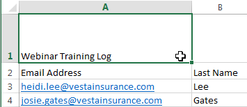
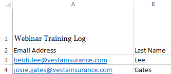
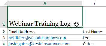
By default, the font of each new workbook is set to Calibri. However, Excel provides many other fonts you can use to customize your cell text. In the example below, we’ll format our title cell to help distinguish it from the rest of the worksheet.
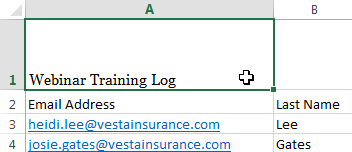
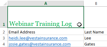
- Select the cell(s) you want to modify.
 Selecting a cell
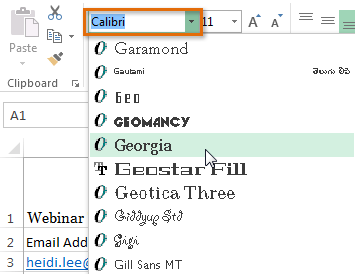
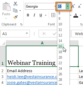
 - Click the drop-down arrow next to the Font command on the Home tab. The Font drop-down menu will appear.
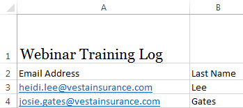
- Select the desired font. A live preview of the new font will appear as you hover the mouse over different options. In our example, we’ll choose Georgia.
 Choosing a font
 - The text will change to the selected font.
 The new font
When creating a workbook in the workplace, you’ll want to select a font that is easy to read. Along with Calibri, standard reading fonts include Cambria, Times New Roman, and Arial.
To change the font size:
- Select the cell(s) you want to modify.
 Selecting a cell
 - Click the drop-down arrow next to the Font Size command on the Home tab. The Font Size drop-down menu will appear.
- Select the desired font size. A live preview of the new font size will appear as you hover the mouse over different options. In our example, we will choose 16 to make the text larger.
 Choosing a new font size
 - The text will change to the selected font size.
 The new font size
You can also use the Increase Font Size and Decrease Font Size commands or enter a custom font size using your keyboard.
 Modifying the font size
To change the font color:
- Select the cell(s) you want to modify.
 Selecting a cell
 - Click the drop-down arrow next to the Font Color command on the Home tab. The Color menu will appear.
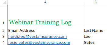
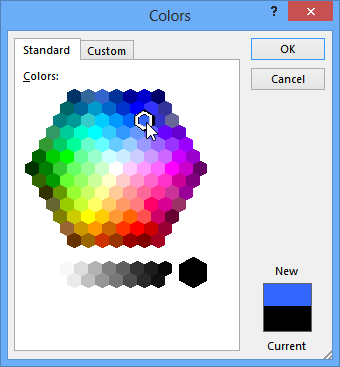
- Select the desired font color. A live preview of the new font color will appear as you hover the mouse over different options. In our example, we’ll choose Green.
 Choosing a font color
 - The text will change to the selected font color.
 The new font color
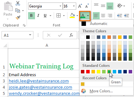
Select More Colors at the bottom of the menu to access additional color options.
 Selecting more colors
To use the Bold, Italic, and Underline commands:
- Select the cell(s) you want to modify.
 Selecting a cell
 - Click the Bold (B), Italic (I), or Underline (U) command on the Home tab. In our example, we’ll make the selected cells bold.
 Clicking the Bold command
 - The selected style will be applied to the text.
The bold text
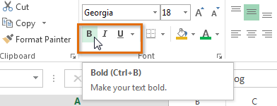
You can also press Ctrl+B on your keyboard to make selected text bold, Ctrl+I to apply italics, and Ctrl+U to apply an underline.
Text alignment
By default, any text entered into your worksheet will be aligned to the bottom-left of a cell, while any numbers will be aligned to the bottom-right. Changing the alignment of your cell content allows you to choose how the content is displayed in any cell, which can make your cell content easier to read.
Click the arrows in the slideshow below to learn more about the different text alignment options.
-
Left align: Aligns content to the left border of the cell
-
Center align: Aligns content an equal distance from the left and right borders of the cell
-
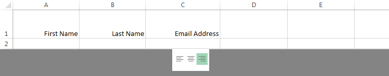
Right Align: Aligns content to the right border of the cell
-
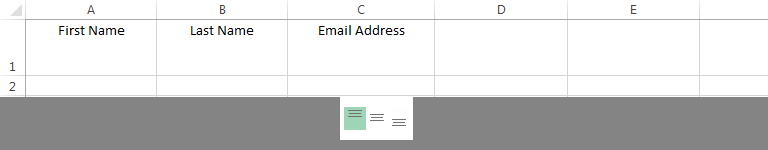
Top Align: Aligns content to the top border of the cell
-
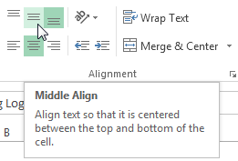
Middle Align: Aligns content an equal distance from the top and bottom borders of the cell
-
Bottom Align: Aligns content to the bottom border of the cell
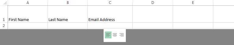
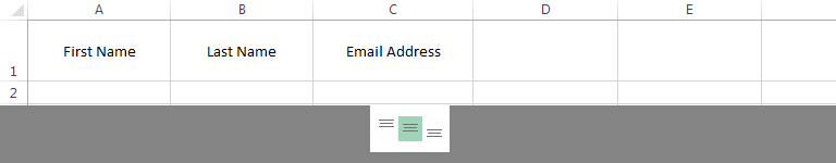
To change horizontal text alignment:
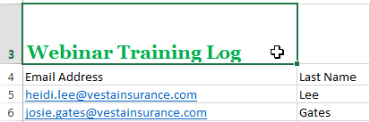
In our example below, we’ll modify the alignment of our title cell to create a more polished look and further distinguish it from the rest of the worksheet.
- Select the cell(s) you want to modify.
 Selecting a cell
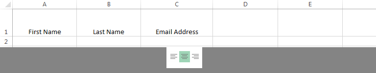
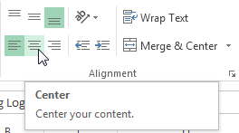
 - Select one of the three horizontal alignment commands on the Home tab. In our example, we’ll choose Center Align.
 Choosing Center Align
 - The text will realign.
 The realigned cell text
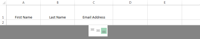
To change vertical text alignment:
- Select the cell(s) you want to modify.
 Selecting a cell
 - Select one of the three vertical alignment commands on the Home tab. In our example, we’ll choose Middle Align.
 Choosing Middle Align
 - The text will realign.
 The realigned cell text
You can apply both vertical and horizontal alignment settings to any cell.
Cell borders and fill colors
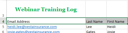
Cell borders and fill colors allow you to create clear and defined boundaries for different sections of your worksheet. Below, we’ll add cell borders and fill color to our header cells to help distinguish them from the rest of the worksheet.
To add a border:
- Select the cell(s) you want to modify.
 Selecting a cell range
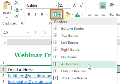
 - Click the drop-down arrow next to the Borders command on the Home tab. The Borders drop-down menu will appear.
- Select the border style you want to use. In our example, we will choose to display All Borders.
 Choosing a border style
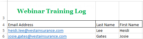
 - The selected border style will appear.
 The added cell borders
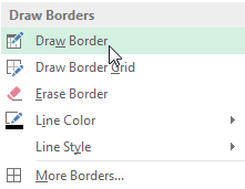
You can draw borders and change the line style and color of borders with the Draw Borders tools at the bottom of the Borders drop-down menu.
 Drawing custom borders
To add a fill color:
- Select the cell(s) you want to modify.
 Selecting a cell range
 - Click the drop-down arrow next to the Fill Color command on the Home tab. The Fill Color menu will appear.
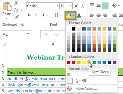
- Select the fill color you want to use. A live preview of the new fill color will appear as you hover the mouse over different options. In our example, we’ll choose Light Green.
 Choosing a cell fill color
 - The selected fill color will appear in the selected cells.
 The new fill color
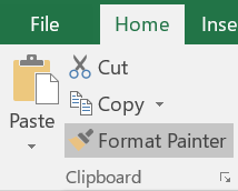
Format Painter
If you want to copy formatting from one cell to another, you can use the Format Painter command on the Home tab. When you click the Format Painter, it will copy all of the formatting from the selected cell. You can then click and drag over any cells you want to paste the formatting to.
Watch the video below to learn two different ways to use the Format Painter.
Cell styles
Instead of formatting cells manually, you can use Excel’s predesigned cell styles. Cell styles are a quick way to include professional formatting for different parts of your workbook, such as titles and headers.
To apply a cell style:
In our example, we’ll apply a new cell style to our existing title and header cells.
- Select the cell(s) you want to modify.
 Selecting a cell range
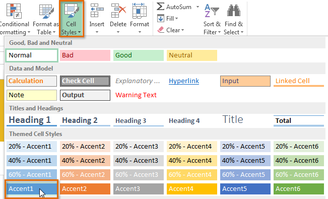
 - Click the Cell Styles command on the Home tab, then choose the desired style from the drop-down menu. In our example, we’ll choose Accent 1.
 Choosing a cell style
 - The selected cell style will appear.
 The new cell style

Applying a cell style will replace any existing cell formatting except for text alignment. You may not want to use cell styles if you’ve already added a lot of formatting to your workbook.
Formatting text and numbers
One of the most powerful tools in Excel is the ability to apply specific formatting for text and numbers. Instead of displaying all cell content in exactly the same way, you can use formatting to change the appearance of dates, times, decimals, percentages (%), currency ($), and much more.
To apply number formatting:
In our example, we’ll change the number format for several cells to modify the way dates are displayed.
- Select the cells(s) you want to modify.
 Selecting a cell range
 - Click the drop-down arrow next to the Number Format command on the Home tab. The Number Formatting drop-down menu will appear.
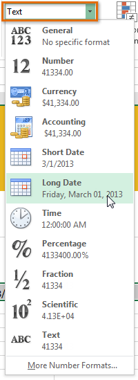
- Select the desired formatting option. In our example, we will change the formatting to Long Date.
 Choosing Long Date
 - The selected cells will change to the new formatting style. For some number formats, you can then use the Increase Decimal and Decrease Decimal commands (below the Number Format command) to change the number of decimal places that are displayed.
 The applied number formatting
Click the buttons in the interactive below to learn about different text and number formatting options.
Challenge!
- Open an existing Excel 2013 workbook. If you want, you can use our practice workbook.
- Select a cell and change the font style, size, and color of the text. If you are using the example, change the title in cell A3 to Verdana font style, size 16, with a font color of green.
- Apply bold, italics, or underline to a cell. If you are using the example, bold the text in cell range A4:C4.
- Try changing the vertical and horizontal text alignment for some cells.
- Add a border to a cell range. If you are using the example, add a border to the header cells in in row 4.
- Change the fill color of a cell range. If you are using the example, add a fill color to row 4.
- Try changing the formatting of a number. If you are using the example, change the date formatting in cell range D4:H4 to Long Date.
/en/excel2013/worksheet-basics/content/
Formatting
Excel has many ways to format and style a spreadsheet.
Why format and style your spreadsheet?
- Make it easier to read and understand
- Make it more delicate
Styling is about changing the looks of cells, such as changing colors, font, font sizes, borders, number formats, and so on.
The most used styling functions are:
- Colors
- Fonts
- Borders
- Number formats
- Grids
There are two ways to access the styling commands in Excel:
- The Ribbon
- Formatting menu, by right clicking cells
Read more about the Ribbon in the Excel overview chapter.
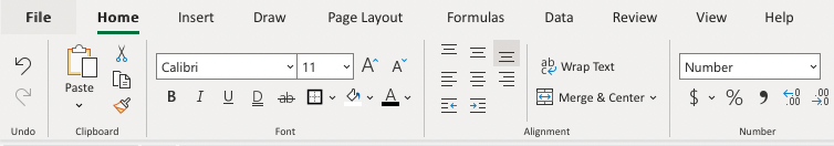
Styling Commands in Ribbon

The Ribbon can be expanded by clicking the arrow/caret-down icon on the right side. This gives access to more commands:

Styling Commands, Right Clicking Cells
You can also right-click on any cell to style it:
Styling commands can be accessed from both views.
Chapter summary
Formatting is used to make spreadsheets more readable. There are many ways to add styles. The most common ones are; Color, Font, Number format and Grids.