
Find and remove duplicates
Excel for Microsoft 365 Excel 2021 Excel 2019 Excel 2016 Excel 2013 Excel 2010 Excel 2007 Excel Starter 2010 More…Less
Sometimes duplicate data is useful, sometimes it just makes it harder to understand your data. Use conditional formatting to find and highlight duplicate data. That way you can review the duplicates and decide if you want to remove them.
-
Select the cells you want to check for duplicates.
Note: Excel can’t highlight duplicates in the Values area of a PivotTable report.
-
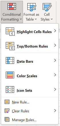
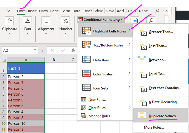
Click Home > Conditional Formatting > Highlight Cells Rules > Duplicate Values.

-
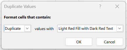
In the box next to values with, pick the formatting you want to apply to the duplicate values, and then click OK.
Remove duplicate values
When you use the Remove Duplicates feature, the duplicate data will be permanently deleted. Before you delete the duplicates, it’s a good idea to copy the original data to another worksheet so you don’t accidentally lose any information.
-
Select the range of cells that has duplicate values you want to remove.
-
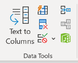
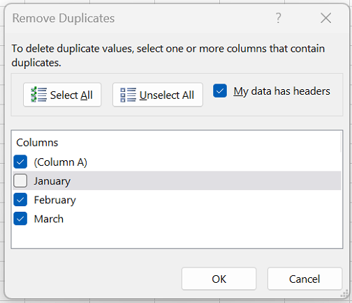
Click Data > Remove Duplicates, and then Under Columns, check or uncheck the columns where you want to remove the duplicates.
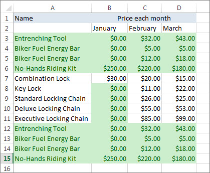
For example, in this worksheet, the January column has price information I want to keep.
So, I unchecked January in the Remove Duplicates box.
-
Click OK.
Note: The counts of duplicate and unique values given after removal may include empty cells, spaces, etc.
Need more help?

Need more help?
Want more options?
Explore subscription benefits, browse training courses, learn how to secure your device, and more.
Communities help you ask and answer questions, give feedback, and hear from experts with rich knowledge.
The easiest way is probably with VLOOKUP(). This will require the 2nd worksheet to have the employee number column sorted though. In newer versions of Excel, apparently sorting is no longer required.
For example, if you had a «Sheet2» with two columns — A = the employee number, B = the employee’s name, and your current worksheet had employee numbers in column D and you want to fill in column E, in cell E2, you would have:
=VLOOKUP($D2, Sheet2!$A$2:$B$65535, 2, FALSE)
Then simply fill this formula down the rest of column D.
Explanation:
- The first argument
$D2specifies the value to search for. - The second argument
Sheet2!$A$2:$B$65535specifies the range of cells to search in. Excel will search for the value in the first column of this range (in this caseSheet2!A2:A65535). Note I am assuming you have a header cell in row 1. - The third argument
2specifies a 1-based index of the column to return from within the searched range. The value of2will return the second column in the rangeSheet2!$A$2:$B$65535, namely the value of theBcolumn. - The fourth argument
FALSEsays to only return exact matches.
Содержание
- How to Tell if Two Cells in Excel Contain the Same Value
- How to Check for Duplicate Cells using the Exact Function
- How to Use the Exact Excel Function to Check for Duplicates
- How to Check Excel for Duplicate Cells using the IF Function
- How to Find Matching Values in Excel
- What’s An Excel Function?
- The Exact Function
- The MATCH Function
- The VLOOKUP Function
- How Do I Find Matching Values in Two Different Sheets?
- How Else Can I Use These Functions?
- Use Excel built-in functions to find data in a table or a range of cells
- Summary
- Create the Sample Worksheet
- Term Definitions
- Functions
- LOOKUP()
- VLOOKUP()
- INDEX() and MATCH()
- OFFSET() and MATCH()
How to Tell if Two Cells in Excel Contain the Same Value
Many companies still use Excel as it allows them to store different types of data, such as tax records and business contacts. Since many things are often done manually in Excel, there is a potential risk of storing duplicate information. It’s usually not an intentional act; it just happens when entering data with a typo, such as a name, account number, amount, or even an address.
Typos or misspellings often lead to new entries when existing data already exists. For instance, your records may have data for John Doe, Jon Dow, or Jon Dow, even though they are the same person.
Making these kinds of mistakes can sometimes lead to grave consequences. That’s precisely why accuracy is so important when working in spreadsheets. Thankfully, Excel includes features and tools that help everyday users check their data and correct errors.
This article shows you how to check whether two or more Excel cells have the same value.
How to Check for Duplicate Cells using the Exact Function
If you want to check whether or not two or more cells have the same value but don’t want to go through the whole table manually, you can make Excel do the work for you. Excel has a built-in function called “Exact.” This function works for both numbers and text.
How to Use the Exact Excel Function to Check for Duplicates
Let’s say you are working with the worksheet shown in the picture below. As you can see, it isn’t easy to determine whether the numbers from column A are the same as any numbers found in column B. Of course, it’s easier than comparing different cells from each column, but you get the idea.

To ensure that cells from column “A” don’t have a duplicate entry in the corresponding column “B” cells, use the “Exact” function, such as checking cells “A1” and “B1” by adding the formula to cell “C1.”
- Click on the “Formulas” tab, then select the “Text” button.
- Choose “EXACT” from the drop-down menu. The “Exact” formula works on numbers as well.
- A window called “Function Arguments” appears. You need to specify which cells you want to compare.
- To compare cells “A1” and “B1,” type “A1” in the “Text1” box and then “B1” in the “Text2” box, then click “OK.”
- Since the numbers from cells “A1” and “B1” don’t match, Excel returns a “FALSE” value and stores the result in cell “C1.”
- To check all cells, drag the “fill handle” (small square in the bottom-right corner of the cell) down the column as far as needed. This action copies and applies an adjusted formula to all other rows.
- After copying the formula down the column, you should notice that the “FALSE” value appears for non-duplicates in each row, and “TRUE” appears for identical ones.


How to Check Excel for Duplicate Cells using the IF Function
Another function that allows you to check two or more cells for duplicates is the “IF” function. It compares cells from one column, row by row. Let’s use the same two columns (A1 and B1) as in the previous example.
To use the “IF” function correctly, remember its syntax.
- In cell “C1,” type the following formula: =IF(A1=B1, “Match”, “”), and you’ll see “Match” next to the cells that have duplicate entries.
- To check for differences, you should type the following formula: =IF(A1<>B1, “No match”,” “). Again, use the fill handle by dragging it down to apply the function to all cells.
- Excel also allows you to check for duplicates and differences simultaneously by typing the following formula: =IF (A1=B1, “No Match”, “Match“) .


In closing, checking for duplicates in Excel is relatively easy when you implement formulas. The human eyes sometimes overlook identical cells, especially when there are hundreds of them to compare. Also, using formulas builds on efficiency and reduces fatigue, not to mention eye strain. These are the easiest methods to find out whether two cells have the same value in Excel.
Of course, there are times when duplicate cells are valid entries, such as dollar amounts for more than one account, two different family members with the same name, or even repeat transactions. Therefore, check the entries before taking action on them, and make a copy first to prevent data loss if something goes wrong.
Источник
How to Find Matching Values in Excel
Ladies and gentlemen, introducing the Exact function
You’ve got an Excel workbook with thousands of numbers and words. There are bound to be multiples of the same number or word in there. You might need to find them. So we’re going to look at several ways you can find matching values in Excel 365.
We’re going to cover finding the same words or numbers in two different worksheets and in two different columns. We’ll look at using the EXACT, MATCH, and VLOOKUP functions. Some of the methods we’ll use may not work in the web version of Microsoft Excel, but they will all work in the desktop version.
What’s An Excel Function?
If you’ve used functions before, skip ahead.
An Excel function is like a mini app. It applies a series of steps to perform a single task. The most commonly used Excel functions can be found in the Formulas tab. Here we see them categorized by the nature of the function –
- AutoSum
- Recently Used
- Financial
- Logical
- Text
- Date & Time
- Lookup & Reference
- Math & Trig
- More Functions.
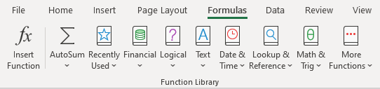
The More Functions category contains the categories Statistical, Engineering, Cube, Information, Compatibility, and Web.
The Exact Function
The Exact function’s task is to go through the rows of two columns and find matching values in the Excel cells. Exact means exact. On its own, the Exact function is case sensitive. It won’t see New York and new york as being a match.
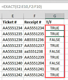
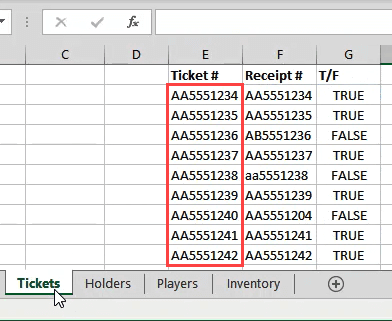
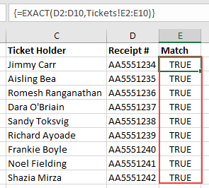
In the example below, there are two columns of text – Tickets and Receipts. For only 10 sets of text, we could compare them by looking at them. Imagine if there were 1,000 rows or more though. That’s when you would use the Exact function.
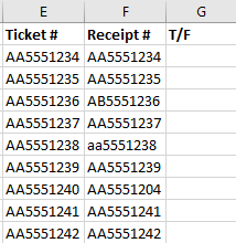
Place the cursor in cell C2. In the formula bar, enter the formula
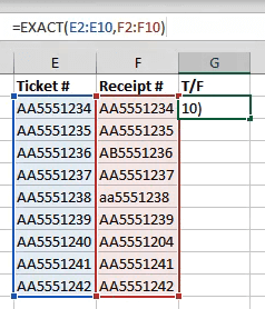
E2:E10 refers to the first column of values and F2:F10 refers to the column right next to it. Once we press Enter, Excel will compare the two values in each row and tell us if it’s a match (True) or not (False). Since we used ranges instead of just two cells, the formula will spill over into the cells below it and evaluate all the other rows.
This method is limited though. It will only compare two cells that are on the same row. It won’t compare what’s in A2 with B3 for example. How do we do that? MATCH can help.
The MATCH Function
MATCH can be used to tell us where a match for a specific value is in a range of cells.
Let’s say we want to find out what row a specific SKU (Stock Keeping Unit) is in, in the example below.
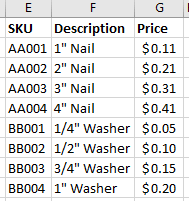
If we want to find what row AA003 is in, we would use the formula:
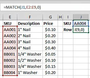
J1 refers to the cell with the value we want to match. E2:E9 refers to the range of values we’re searching through. The zero (0) at the end of the formula tells Excel to look for an exact match. If we were matching numbers, we could use 1 to find something less than our query or 2 to find something greater than our query.
But what if we wanted to find the price of AA003?
The VLOOKUP Function
The V in VLOOKUP stands for vertical. Meaning it can search for a given value in a column. What it can also do is return a value on the same row as the found value.
If you’ve got an Office 365 subscription in the Monthly channel, you can use the newer XLOOKUP. If you only have the semi-annual subscription it will be available to you in July 2020.
Let’s use the same inventory data and try to find the price of something.

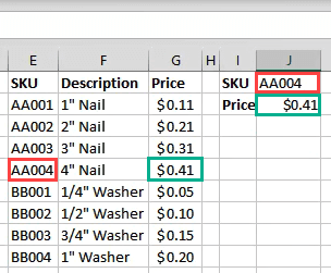
Where we were looking for a row before, enter the formula:
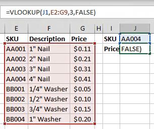
J1 refers to the cell with the value we’re matching. E2:G9 is the range of values we’re working with. But VLOOKUP will only look in the first column of that range for a match. The 3 refers to the 3rd column over from the start of the range.
So when we type a SKU in J1, VLOOKUP will find the match and grab the value from the cell 3 columns over from it. FALSE tells Excel what kind of match we’re looking for. FALSE means it must be an exact match where TRUE would tell it that it has to be a close match.
How Do I Find Matching Values in Two Different Sheets?
Each of the functions above can work across two different sheets to find matching values in Excel. We’re going to use the EXACT function to show you how. This can be done with almost any function. Not just the ones we covered here. There are also other ways to link cells between different sheets and workbooks.
Working on the Holders sheet, we enter the formula
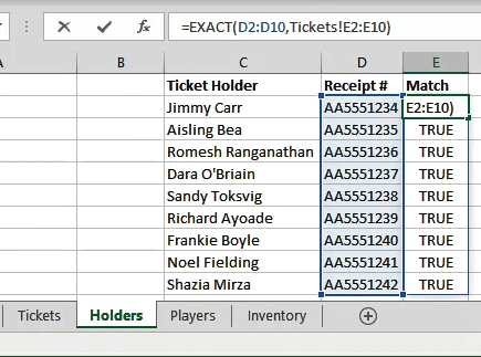
D2:D10 is the range we’ve selected on the Holders sheet. Once we put a comma after that, we can click on the Tickets sheet and drag and select the second range.
See how it references the sheet and range as Tickets!E2:E10? In this case each row matches, so the results are all True.
How Else Can I Use These Functions?
Once you master these functions for matching and finding things, you can start doing a lot of different things with them. Also take a look at using the INDEX and MATCH functions together to do something similar to VLOOKUP.
Have some cool tips on using Excel functions to find matching values in Excel? Maybe a question about how to do more? Drop us a note in the comments below.
Guy has been published online and in print newspapers, nominated for writing awards, and cited in scholarly papers due to his ability to speak tech to anyone, but still prefers analog watches. Read Guy’s Full Bio
Источник
Use Excel built-in functions to find data in a table or a range of cells
Summary
This step-by-step article describes how to find data in a table (or range of cells) by using various built-in functions in Microsoft Excel. You can use different formulas to get the same result.
Create the Sample Worksheet
This article uses a sample worksheet to illustrate Excel built-in functions. Consider the example of referencing a name from column A and returning the age of that person from column C. To create this worksheet, enter the following data into a blank Excel worksheet.
You will type the value that you want to find into cell E2. You can type the formula in any blank cell in the same worksheet.
Term Definitions
This article uses the following terms to describe the Excel built-in functions:
The whole lookup table
The value to be found in the first column of Table_Array.
Lookup_Array
-or-
Lookup_Vector
The range of cells that contains possible lookup values.
The column number in Table_Array the matching value should be returned for.
3 (third column in Table_Array)
Result_Array
-or-
Result_Vector
A range that contains only one row or column. It must be the same size as Lookup_Array or Lookup_Vector.
A logical value (TRUE or FALSE). If TRUE or omitted, an approximate match is returned. If FALSE, it will look for an exact match.
This is the reference from which you want to base the offset. Top_Cell must refer to a cell or range of adjacent cells. Otherwise, OFFSET returns the #VALUE! error value.
This is the number of columns, to the left or right, that you want the upper-left cell of the result to refer to. For example, «5» as the Offset_Col argument specifies that the upper-left cell in the reference is five columns to the right of reference. Offset_Col can be positive (which means to the right of the starting reference) or negative (which means to the left of the starting reference).
Functions
LOOKUP()
The LOOKUP function finds a value in a single row or column and matches it with a value in the same position in a different row or column.
The following is an example of LOOKUP formula syntax:
The following formula finds Mary’s age in the sample worksheet:
The formula uses the value «Mary» in cell E2 and finds «Mary» in the lookup vector (column A). The formula then matches the value in the same row in the result vector (column C). Because «Mary» is in row 4, LOOKUP returns the value from row 4 in column C (22).
NOTE: The LOOKUP function requires that the table be sorted.
For more information about the LOOKUP function, click the following article number to view the article in the Microsoft Knowledge Base:
VLOOKUP()
The VLOOKUP or Vertical Lookup function is used when data is listed in columns. This function searches for a value in the left-most column and matches it with data in a specified column in the same row. You can use VLOOKUP to find data in a sorted or unsorted table. The following example uses a table with unsorted data.
The following is an example of VLOOKUP formula syntax:
The following formula finds Mary’s age in the sample worksheet:
The formula uses the value «Mary» in cell E2 and finds «Mary» in the left-most column (column A). The formula then matches the value in the same row in Column_Index. This example uses «3» as the Column_Index (column C). Because «Mary» is in row 4, VLOOKUP returns the value from row 4 in column C (22).
For more information about the VLOOKUP function, click the following article number to view the article in the Microsoft Knowledge Base:
INDEX() and MATCH()
You can use the INDEX and MATCH functions together to get the same results as using LOOKUP or VLOOKUP.
The following is an example of the syntax that combines INDEX and MATCH to produce the same results as LOOKUP and VLOOKUP in the previous examples:
The following formula finds Mary’s age in the sample worksheet:
The formula uses the value «Mary» in cell E2 and finds «Mary» in column A. It then matches the value in the same row in column C. Because «Mary» is in row 4, the formula returns the value from row 4 in column C (22).
NOTE: If none of the cells in Lookup_Array match Lookup_Value («Mary»), this formula will return #N/A.
For more information about the INDEX function, click the following article number to view the article in the Microsoft Knowledge Base:
OFFSET() and MATCH()
You can use the OFFSET and MATCH functions together to produce the same results as the functions in the previous example.
The following is an example of syntax that combines OFFSET and MATCH to produce the same results as LOOKUP and VLOOKUP:
This formula finds Mary’s age in the sample worksheet:
The formula uses the value «Mary» in cell E2 and finds «Mary» in column A. The formula then matches the value in the same row but two columns to the right (column C). Because «Mary» is in column A, the formula returns the value in row 4 in column C (22).
For more information about the OFFSET function, click the following article number to view the article in the Microsoft Knowledge Base:
Источник
![]()
Find Duplicates in Excel

It is very easy to find duplicates in Excel. We can use built in tools (Conditional Formats, Filters) or formula (COUNTIF or VLOOKUP) to find duplicates in Excel Columns or Rows. Let us see the best and easy methods to find duplicate values in Excel.
Find duplicates Using Conditional Formatting
We can easily identify the duplicates using Conditional Formatting Tools in Excel. We can select the range and highlight the duplicate values with color. Following are the different methods to find duplicate entries in excel and strikethrough the duplicates using Conditional Formatting.
Highlighting duplicate values in Excel
We can highlight the duplicate values in the Excel with specific color. We can change the fill color and font color for the duplicate values. Please follow the below steps to identify the duplicates.
- Select the required range of cell to find duplicates
- Go to ‘Home’ Tab in the Ribbon Menu
- Click on the ‘Conditional Formatting’ command
- Go to ‘Highlight Cells Rules’ and Click on ‘Duplicate Values…’
- And Choose the formatting Options from the drop down list and Click on ‘OK’
Now you can see that all the duplicate values are highlighted as shown in the screen-shot.
Strike through duplicate values in Excel
We can strike through the duplicate values in the Excel. It is very helpful to strike out all duplicate entries in a range of cells. We can use the conditional formatting command in Excel to strike through the duplicate Cells.

- Select the required range of cell to strike through the duplicates
- Go to ‘Home’ Tab in the Ribbon
- Click on the ‘Conditional Formatting’ command
- Go to ‘Highlight Cells Rules’ and Click on ‘Duplicate Values…’
- And Choose the Custom Format from formatting Options from the drop down list
- Select the Strikethrough option from Font effects and Click on ‘OK’
Now you can see that all the duplicate values are stroked out as shown in the screen-shot.
Formula for checking duplicates
We can create formula using COUNTIF or VLOOKUP Functions to check the duplicates in Excel. Following is the step by explanation for finding duplicate values using Excel Formula.
Finding Duplicates using COUNTIF Formula
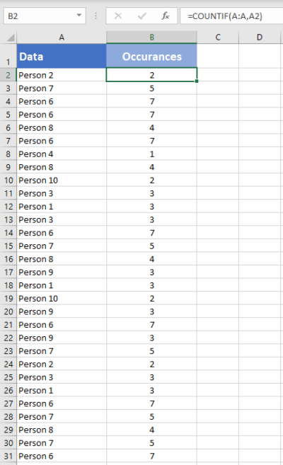
We can use COUNTIF Formula in Excel Cells to identify duplicates in Excel. COUNTIF formula helps to find duplicates in One Column, returns the number of occurrences of a given value. We can identify the duplicates if the Count is greater than 1. We can create new column to mark the duplicates using Excel COUNTIF Formula.
You can see that we have enter the COUNTIF formula in Range B2 to check the total occurrences of A1 value in the entire Column A:A.This will return the frequency of each Cell value of Column A in Column B.
We can identify the duplicate Cells based on the value in the Column B. If the values is greater than 1, we confirm that the values contains duplicate entries in the specified range or column.
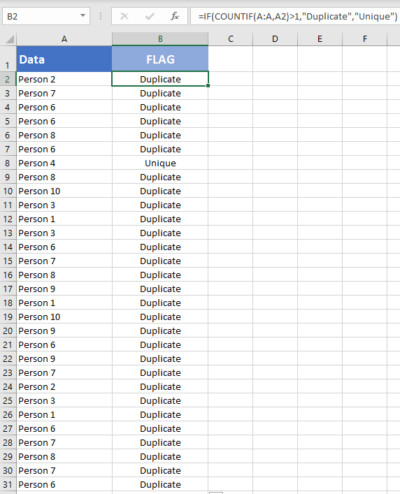
Mark Duplicates and Unique Entries using Formula
We can enhance the above formula to mark all duplicates in a Column. The following formula will return ‘Duplicate’ if the cell value contains duplicate values, otherwise returns ‘Unique’.
=IF(COUNTIF(A:A,A2)>1,"Duplicate","Unique")
Formula will return ‘Duplicate’ in the Column B if the value repeats (count >1).
It will return ‘Unique’ in the Column B if the count is 1.
Find duplicate values in excel using VLookup
We can use VLOOKUP formula to compare two columns (or lists) and find the duplicate values. Vlookup helps to find duplicates in Two Column and duplicate rows based on Multiple Columns. Following are steps to find duplicates using VLOOKUP function.
We have two lists in the Excel List 1 in Column A and List 2 in Column B. Let us find the duplicate values in the List 2 which are part of List 1.
=VLOOKUP(B2,$A$2:$A$15,1,FALSE)
VLOOKUP Formula will check for the Cell B2 value in the specified Range (A2:A5) and Returns the value if found, it will return #NA if it is not found in List 1. We can confirm if the the value is duplicated in List 1 and 2 if it returns the Value, it will be unique if it returns #NA.

How to find duplicate values in Excel using VlookUp?
You can use Excel formula to find the duplicate values in Excel by using vlookup formula as described below. You can use the Excel VlookUp to identify the duplicates in Excel.
=IF(ISNA(VLOOKUP(B2,$A$2:$A$15,1,FALSE)),"Unique","Duplicate")
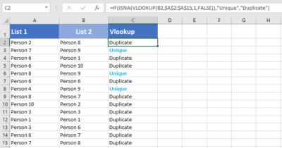
We can enhance this formula to identify the duplicates and unique values in the Column 2. We can use the Excel IF and ISNA Formulas along with VLOOKUP to return the required Labels.
You can use this method to compare with other worksheets and find duplicate values in Different Excel Sheets.
How to find duplicate values in two columns in excel using VlookUp?
Follow the below steps to find the duplicate values in two columns in excel using VlookUp. We generally need this to compare two columns and check if a value is existing in two columns.
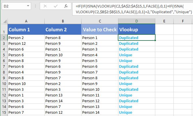
=IF(IF(ISNA(VLOOKUP(C2,$A$2:$A$15,1,FALSE)),0,1)
+IF(ISNA(VLOOKUP(C2,$B$2:$B$15,1,FALSE)),0,1)=2,"Duplicated","Unique")
Here, we have Two Target Columns A and B , we check if the items in Column C are duplicated or not.
If you wants to compare two columns and check for values are repeated in both the columns or not, you can use this formula.
Share This Story, Choose Your Platform!
2 Comments
-
Guru
August 12, 2019 at 7:45 pm — ReplyThanks for very useful instructions to check duplicates in Excel.
-
Tom
August 12, 2019 at 7:48 pm — ReplyThis is very clear and simple! Thanks a lot for providing clear help to identify the duplicates in Excel.
© Copyright 2012 – 2020 | Excelx.com | All Rights Reserved
Page load link
The searching of duplicates in Excel – is one of the most common tasks for any of office employee. For its solution, there are a few different methods. But – how quickly to find duplicates in Excel and to highlight them with color? For the answer on this frequently asked question let us consider a concrete example.
How to find duplicate values in Excel?
For example we are engaging by check orders, which coming into the firm through Fax and e-mail. There can be such situation that the same order was by the two channels of incoming information. If you register twice the same order, there can be certain problems for the firm. Below we are considering to the decision by means of the conditional formatting.
For avoiding of the duplicate orders, you can use to the conditional formatting, which helps you quickly to find the duplicate values in Excel column.
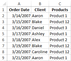
The example of the day orders for goods:
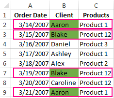
For verification whether the day orders are possible duplicates, we will analyze in the names of customers – there is the column B:
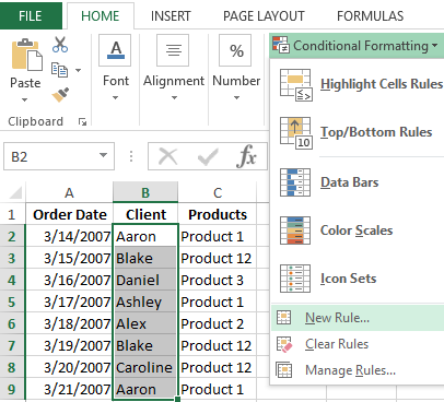
- To highlight the range B2:B9 and then to select the instrument: «HOME» — «Styles» — «Conditional Formatting» — «New Rule».
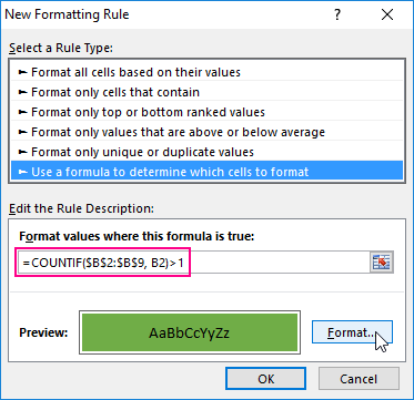
- To choose «Use a formula to determine which cells to format».
- To find the duplicate values in Excel column, you need to enter the formula in the input field:
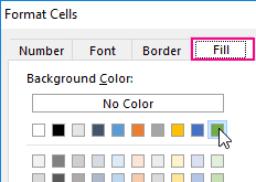
- After that you need to press the button «Format» and select to the desired cell shading to highlight duplicates in color — for example, green one. And click OK on all windows are opened.
Download an example of finding the Identifying Duplicate values in a column.
As can be seen in the picture with the conditional formatting we were able easily and quickly to implement the duplicate finder in function Excel and to detect to the duplicate data cells for the table of the day orders.
The example of COUNTIF function and highlighting of the duplicate values
The principle of the action formula for finding of the duplicates by the conditional formatting is simple. The formula contains the function =COUNTIF(). This function can also be used when searching for the identical values in the range of cells. The first argument in the function to the viewable data range is specified. In the second argument we specify what we are looking for. The first argument has an absolute reference, as it should be the same one. And the second argument conversely — should be changed on the address of the each cell in the viewing range, because it has a relative link one.
The fastest and the simplest ways: to find to the duplicates in the cells.
After the function we can see the comparison operator of the number of the found values in the range with the number 1. That is, if we see more, than one value means that the formula returns the value of TRUE and for the current cell is applied to the conditional formatting.