Excel find which row - Word и Excel - помощь в работе с программами

Содержание

LOOKUP function
There are two ways to use LOOKUP: Vector form and Array form
Vector form
Syntax
Remarks
Vector examples
Array form
Syntax
Use Excel built-in functions to find data in a table or a range of cells
Summary
Create the Sample Worksheet
Term Definitions
Functions
LOOKUP()
VLOOKUP()
INDEX() and MATCH()
OFFSET() and MATCH()
Find the ROW number in excel with multiple matching criteria
2 Answers 2
Look up values with VLOOKUP, INDEX, or MATCH
Using INDEX and MATCH instead of VLOOKUP
Give it a try
VLOOKUP Example at work

LOOKUP function

Use LOOKUP, one of the lookup and reference functions, when you need to look in a single row or column and find a value from the same position in a second row or column.

For example, let’s say you know the part number for an auto part, but you don’t know the price. You can use the LOOKUP function to return the price in cell H2 when you enter the auto part number in cell H1.

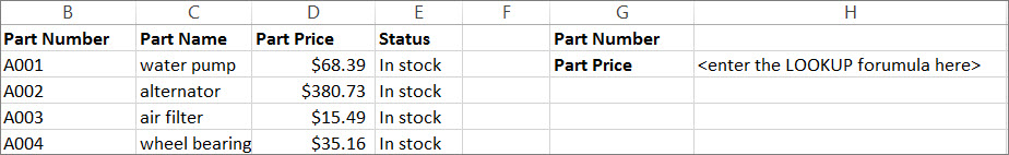
Use the LOOKUP function to search one row or one column. In the above example, we’re searching prices in column D.

Tips: Consider one of the newer lookup functions, depending on which version you are using.

Use VLOOKUP to search one row or column, or to search multiple rows and columns (like a table). It’s a much improved version of LOOKUP. Watch this video about how to use VLOOKUP.

If you are using Microsoft 365, use XLOOKUP — it’s not only faster, it also lets you search in any direction (up, down, left, right).

There are two ways to use LOOKUP: Vector form and Array form

Vector form: Use this form of LOOKUP to search one row or one column for a value. Use the vector form when you want to specify the range that contains the values that you want to match. For example, if you want to search for a value in column A, down to row 6.

Array form: We strongly recommend using VLOOKUP or HLOOKUP instead of the array form. Watch this video about using VLOOKUP. The array form is provided for compatibility with other spreadsheet programs, but it’s functionality is limited.

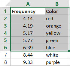
An array is a collection of values in rows and columns (like a table) that you want to search. For example, if you want to search columns A and B, down to row 6. LOOKUP will return the nearest match. To use the array form, your data must be sorted.

Vector form

The vector form of LOOKUP looks in a one-row or one-column range (known as a vector) for a value and returns a value from the same position in a second one-row or one-column range.

Syntax

LOOKUP(lookup_value, lookup_vector, [result_vector])

The LOOKUP function vector form syntax has the following arguments:

lookup_value Required. A value that LOOKUP searches for in the first vector. Lookup_value can be a number, text, a logical value, or a name or reference that refers to a value.

lookup_vector Required. A range that contains only one row or one column. The values in lookup_vector can be text, numbers, or logical values.

Important: The values in lookup_vector must be placed in ascending order: . -2, -1, 0, 1, 2, . A-Z, FALSE, TRUE; otherwise, LOOKUP might not return the correct value. Uppercase and lowercase text are equivalent.

result_vector Optional. A range that contains only one row or column. The result_vector argument must be the same size as lookup_vector. It has to be the same size.

If the LOOKUP function can’t find the lookup_value, the function matches the largest value in lookup_vector that is less than or equal to lookup_value.

If lookup_value is smaller than the smallest value in lookup_vector, LOOKUP returns the #N/A error value.

Vector examples

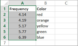
You can try out these examples in your own Excel worksheet to learn how the LOOKUP function works. In the first example, you’re going to end up with a spreadsheet that looks similar to this one:

Copy the data in following table, and paste it into a new Excel worksheet.

Copy this data into column A

Copy this data into column B

Next, copy the LOOKUP formulas from the following table into column D of your worksheet.

Copy this formula into the D column

Here’s what this formula does

Here’s the result you’ll see

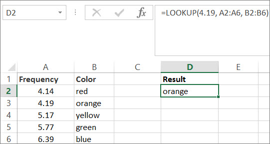
=LOOKUP(4.19, A2:A6, B2:B6)

Looks up 4.19 in column A, and returns the value from column B that is in the same row.

=LOOKUP(5.75, A2:A6, B2:B6)

Looks up 5.75 in column A, matches the nearest smaller value (5.17), and returns the value from column B that is in the same row.

=LOOKUP(7.66, A2:A6, B2:B6)

Looks up 7.66 in column A, matches the nearest smaller value (6.39), and returns the value from column B that is in the same row.

=LOOKUP(0, A2:A6, B2:B6)

Looks up 0 in column A, and returns an error because 0 is less than the smallest value (4.14) in column A.

For these formulas to show results, you may need to select them in your Excel worksheet, press F2, and then press Enter. If you need to, adjust the column widths to see all the data.

Array form

Tip: We strongly recommend using VLOOKUP or HLOOKUP instead of the array form. See this video about VLOOKUP; it provides examples. The array form of LOOKUP is provided for compatibility with other spreadsheet programs, but its functionality is limited.

The array form of LOOKUP looks in the first row or column of an array for the specified value and returns a value from the same position in the last row or column of the array. Use this form of LOOKUP when the values that you want to match are in the first row or column of the array.

Syntax

The LOOKUP function array form syntax has these arguments:

lookup_value Required. A value that LOOKUP searches for in an array. The lookup_value argument can be a number, text, a logical value, or a name or reference that refers to a value.

If LOOKUP can’t find the value of lookup_value, it uses the largest value in the array that is less than or equal to lookup_value.

If the value of lookup_value is smaller than the smallest value in the first row or column (depending on the array dimensions), LOOKUP returns the #N/A error value.

array Required. A range of cells that contains text, numbers, or logical values that you want to compare with lookup_value.

The array form of LOOKUP is very similar to the HLOOKUP and VLOOKUP functions. The difference is that HLOOKUP searches for the value of lookup_value in the first row, VLOOKUP searches in the first column, and LOOKUP searches according to the dimensions of array.

If array covers an area that is wider than it is tall (more columns than rows), LOOKUP searches for the value of lookup_value in the first row.

If an array is square or is taller than it is wide (more rows than columns), LOOKUP searches in the first column.

With the HLOOKUP and VLOOKUP functions, you can index down or across, but LOOKUP always selects the last value in the row or column.

Important: The values in array must be placed in ascending order: . -2, -1, 0, 1, 2, . A-Z, FALSE, TRUE; otherwise, LOOKUP might not return the correct value. Uppercase and lowercase text are equivalent.

Источник

Use Excel built-in functions to find data in a table or a range of cells

Summary

This step-by-step article describes how to find data in a table (or range of cells) by using various built-in functions in Microsoft Excel. You can use different formulas to get the same result.

Create the Sample Worksheet

This article uses a sample worksheet to illustrate Excel built-in functions. Consider the example of referencing a name from column A and returning the age of that person from column C. To create this worksheet, enter the following data into a blank Excel worksheet.

You will type the value that you want to find into cell E2. You can type the formula in any blank cell in the same worksheet.

Term Definitions

This article uses the following terms to describe the Excel built-in functions:

The whole lookup table

The value to be found in the first column of Table_Array.

Lookup_Array
-or-
Lookup_Vector

The range of cells that contains possible lookup values.

The column number in Table_Array the matching value should be returned for.

3 (third column in Table_Array)

Result_Array
-or-
Result_Vector

A range that contains only one row or column. It must be the same size as Lookup_Array or Lookup_Vector.

A logical value (TRUE or FALSE). If TRUE or omitted, an approximate match is returned. If FALSE, it will look for an exact match.

This is the reference from which you want to base the offset. Top_Cell must refer to a cell or range of adjacent cells. Otherwise, OFFSET returns the #VALUE! error value.

This is the number of columns, to the left or right, that you want the upper-left cell of the result to refer to. For example, «5» as the Offset_Col argument specifies that the upper-left cell in the reference is five columns to the right of reference. Offset_Col can be positive (which means to the right of the starting reference) or negative (which means to the left of the starting reference).

Functions

LOOKUP()

The LOOKUP function finds a value in a single row or column and matches it with a value in the same position in a different row or column.

The following is an example of LOOKUP formula syntax:

The following formula finds Mary’s age in the sample worksheet:

The formula uses the value «Mary» in cell E2 and finds «Mary» in the lookup vector (column A). The formula then matches the value in the same row in the result vector (column C). Because «Mary» is in row 4, LOOKUP returns the value from row 4 in column C (22).

NOTE: The LOOKUP function requires that the table be sorted.

For more information about the LOOKUP function, click the following article number to view the article in the Microsoft Knowledge Base:

VLOOKUP()

The VLOOKUP or Vertical Lookup function is used when data is listed in columns. This function searches for a value in the left-most column and matches it with data in a specified column in the same row. You can use VLOOKUP to find data in a sorted or unsorted table. The following example uses a table with unsorted data.

The following is an example of VLOOKUP formula syntax:

The following formula finds Mary’s age in the sample worksheet:

The formula uses the value «Mary» in cell E2 and finds «Mary» in the left-most column (column A). The formula then matches the value in the same row in Column_Index. This example uses «3» as the Column_Index (column C). Because «Mary» is in row 4, VLOOKUP returns the value from row 4 in column C (22).

For more information about the VLOOKUP function, click the following article number to view the article in the Microsoft Knowledge Base:

INDEX() and MATCH()

You can use the INDEX and MATCH functions together to get the same results as using LOOKUP or VLOOKUP.

The following is an example of the syntax that combines INDEX and MATCH to produce the same results as LOOKUP and VLOOKUP in the previous examples:

The following formula finds Mary’s age in the sample worksheet:

The formula uses the value «Mary» in cell E2 and finds «Mary» in column A. It then matches the value in the same row in column C. Because «Mary» is in row 4, the formula returns the value from row 4 in column C (22).

NOTE: If none of the cells in Lookup_Array match Lookup_Value («Mary»), this formula will return #N/A.
For more information about the INDEX function, click the following article number to view the article in the Microsoft Knowledge Base:

OFFSET() and MATCH()

You can use the OFFSET and MATCH functions together to produce the same results as the functions in the previous example.

The following is an example of syntax that combines OFFSET and MATCH to produce the same results as LOOKUP and VLOOKUP:

This formula finds Mary’s age in the sample worksheet:

The formula uses the value «Mary» in cell E2 and finds «Mary» in column A. The formula then matches the value in the same row but two columns to the right (column C). Because «Mary» is in column A, the formula returns the value in row 4 in column C (22).

For more information about the OFFSET function, click the following article number to view the article in the Microsoft Knowledge Base:

Источник

Find the ROW number in excel with multiple matching criteria

I need to be able to find the row number of the row where matching criteria from A1 is equal or greater than values in column C and lesser or equal than values in column D

I can use INDEX and MATCH combo but not sure if this is something I should use for multiple criteria matching.

Any help or suggestions are highly appreciated.

2 Answers 2

I would not use MATCH to get the row number since you have multiple criteria. I would still use INDEX however to get the value of the row in E once the proper row number was discovered.

So instead of MATCH I would use an array formula using an IF statement that contained multiple criteria. Now note that array formulas need to be entered using ctrl + shift + enter . The IF statement would look like this:

Note: I did not use the AND formula here because that cannot take in arrays. But since booleans are just 1’s or 0’s in Excel, multiplying the criteria works just fine.

This now gives us an array containing only blanks and valid row numbers. Such that if rows 5 and 7 were both valid the array would look like:

Now if we encapsulate that IF statement with a SMALL we can get whatever valid row we want. In this case since we just want the first valid row we can use:

Which if the first valid row is 5 then that will return 5. Incrementing the K value of the SMALL formula will allow you to grab the 2nd, 3rd, etc valid row.

Now of course since we have the row number a simple INDEX will get us the value in column E:

Источник

Look up values with VLOOKUP, INDEX, or MATCH

Tip: Try using the new XLOOKUP and XMATCH functions, improved versions of the functions described in this article. These new functions work in any direction and return exact matches by default, making them easier and more convenient to use than their predecessors.

Suppose that you have a list of office location numbers, and you need to know which employees are in each office. The spreadsheet is huge, so you might think it is challenging task. It’s actually quite easy to do with a lookup function.

The VLOOKUP and HLOOKUP functions, together with INDEX and MATCH, are some of the most useful functions in Excel.

Note: The Lookup Wizard feature is no longer available in Excel.

Here’s an example of how to use VLOOKUP.

In this example, B2 is the first argument—an element of data that the function needs to work. For VLOOKUP, this first argument is the value that you want to find. This argument can be a cell reference, or a fixed value such as «smith» or 21,000. The second argument is the range of cells, C2-:E7, in which to search for the value you want to find. The third argument is the column in that range of cells that contains the value that you seek.

The fourth argument is optional. Enter either TRUE or FALSE. If you enter TRUE, or leave the argument blank, the function returns an approximate match of the value you specify in the first argument. If you enter FALSE, the function will match the value provide by the first argument. In other words, leaving the fourth argument blank—or entering TRUE—gives you more flexibility.

This example shows you how the function works. When you enter a value in cell B2 (the first argument), VLOOKUP searches the cells in the range C2:E7 (2nd argument) and returns the closest approximate match from the third column in the range, column E (3rd argument).

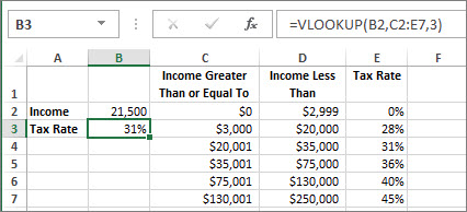
The fourth argument is empty, so the function returns an approximate match. If it didn’t, you’d have to enter one of the values in columns C or D to get a result at all.

When you’re comfortable with VLOOKUP, the HLOOKUP function is equally easy to use. You enter the same arguments, but it searches in rows instead of columns.

Using INDEX and MATCH instead of VLOOKUP

There are certain limitations with using VLOOKUP—the VLOOKUP function can only look up a value from left to right. This means that the column containing the value you look up should always be located to the left of the column containing the return value. Now if your spreadsheet isn’t built this way, then do not use VLOOKUP. Use the combination of INDEX and MATCH functions instead.

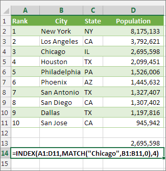
This example shows a small list where the value we want to search on, Chicago, isn’t in the leftmost column. So, we can’t use VLOOKUP. Instead, we’ll use the MATCH function to find Chicago in the range B1:B11. It’s found in row 4. Then, INDEX uses that value as the lookup argument, and finds the population for Chicago in the 4th column (column D). The formula used is shown in cell A14.

For more examples of using INDEX and MATCH instead of VLOOKUP, see the article https://www.mrexcel.com/excel-tips/excel-vlookup-index-match/ by Bill Jelen, Microsoft MVP.

Give it a try

If you want to experiment with lookup functions before you try them out with your own data, here’s some sample data.

VLOOKUP Example at work

Copy the following data into a blank spreadsheet.

Tip: Before you paste the data into Excel, set the column widths for columns A through C to 250 pixels, and click Wrap Text ( Home tab, Alignment group).

Источник

Use LOOKUP, one of the lookup and reference functions, when you need to look in a single row or column and find a value from the same position in a second row or column.

Use the LOOKUP function to search one row or one column. In the above example, we’re searching prices in column D.

Tips: Consider one of the newer lookup functions, depending on which version you are using.

Use VLOOKUP to search one row or column, or to search multiple rows and columns (like a table). It’s a much improved version of LOOKUP. Watch this video about how to use VLOOKUP.
If you are using Microsoft 365, use XLOOKUP — it’s not only faster, it also lets you search in any direction (up, down, left, right).

There are two ways to use LOOKUP: Vector form and Array form

Vector form: Use this form of LOOKUP to search one row or one column for a value. Use the vector form when you want to specify the range that contains the values that you want to match. For example, if you want to search for a value in column A, down to row 6.
Array form: We strongly recommend using VLOOKUP or HLOOKUP instead of the array form. Watch this video about using VLOOKUP. The array form is provided for compatibility with other spreadsheet programs, but it’s functionality is limited.

An array is a collection of values in rows and columns (like a table) that you want to search. For example, if you want to search columns A and B, down to row 6. LOOKUP will return the nearest match. To use the array form, your data must be sorted.

Vector form

The vector form of LOOKUP looks in a one-row or one-column range (known as a vector) for a value and returns a value from the same position in a second one-row or one-column range.

Syntax

LOOKUP(lookup_value, lookup_vector, [result_vector])

The LOOKUP function vector form syntax has the following arguments:

lookup_value Required. A value that LOOKUP searches for in the first vector. Lookup_value can be a number, text, a logical value, or a name or reference that refers to a value.
lookup_vector Required. A range that contains only one row or one column. The values in lookup_vector can be text, numbers, or logical values.

Important: The values in lookup_vector must be placed in ascending order: …, -2, -1, 0, 1, 2, …, A-Z, FALSE, TRUE; otherwise, LOOKUP might not return the correct value. Uppercase and lowercase text are equivalent.
result_vector Optional. A range that contains only one row or column. The result_vector argument must be the same size as lookup_vector. It has to be the same size.

Remarks

If the LOOKUP function can’t find the lookup_value, the function matches the largest value in lookup_vector that is less than or equal to lookup_value.
If lookup_value is smaller than the smallest value in lookup_vector, LOOKUP returns the #N/A error value.

Vector examples

You can try out these examples in your own Excel worksheet to learn how the LOOKUP function works. In the first example, you’re going to end up with a spreadsheet that looks similar to this one:

Copy the data in following table, and paste it into a new Excel worksheet.

Copy this data into column A	Copy this data into column B
Frequency 4.14	Color red
4.19	orange
5.17	yellow
5.77	green
6.39	blue

Next, copy the LOOKUP formulas from the following table into column D of your worksheet.

Copy this formula into the D column	Here’s what this formula does	Here’s the result you’ll see
Formula
=LOOKUP(4.19, A2:A6, B2:B6)	Looks up 4.19 in column A, and returns the value from column B that is in the same row.	orange
=LOOKUP(5.75, A2:A6, B2:B6)	Looks up 5.75 in column A, matches the nearest smaller value (5.17), and returns the value from column B that is in the same row.	yellow
=LOOKUP(7.66, A2:A6, B2:B6)	Looks up 7.66 in column A, matches the nearest smaller value (6.39), and returns the value from column B that is in the same row.	blue
=LOOKUP(0, A2:A6, B2:B6)	Looks up 0 in column A, and returns an error because 0 is less than the smallest value (4.14) in column A.	#N/A

For these formulas to show results, you may need to select them in your Excel worksheet, press F2, and then press Enter. If you need to, adjust the column widths to see all the data.

Array form

The array form of LOOKUP looks in the first row or column of an array for the specified value and returns a value from the same position in the last row or column of the array. Use this form of LOOKUP when the values that you want to match are in the first row or column of the array.

Syntax

LOOKUP(lookup_value, array)

The LOOKUP function array form syntax has these arguments:

lookup_value Required. A value that LOOKUP searches for in an array. The lookup_value argument can be a number, text, a logical value, or a name or reference that refers to a value.
- If LOOKUP can’t find the value of lookup_value, it uses the largest value in the array that is less than or equal to lookup_value.
- If the value of lookup_value is smaller than the smallest value in the first row or column (depending on the array dimensions), LOOKUP returns the #N/A error value.
array Required. A range of cells that contains text, numbers, or logical values that you want to compare with lookup_value.

The array form of LOOKUP is very similar to the HLOOKUP and VLOOKUP functions. The difference is that HLOOKUP searches for the value of lookup_value in the first row, VLOOKUP searches in the first column, and LOOKUP searches according to the dimensions of array.
- If array covers an area that is wider than it is tall (more columns than rows), LOOKUP searches for the value of lookup_value in the first row.
- If an array is square or is taller than it is wide (more rows than columns), LOOKUP searches in the first column.
- With the HLOOKUP and VLOOKUP functions, you can index down or across, but LOOKUP always selects the last value in the row or column.
  
  Important: The values in array must be placed in ascending order: …, -2, -1, 0, 1, 2, …, A-Z, FALSE, TRUE; otherwise, LOOKUP might not return the correct value. Uppercase and lowercase text are equivalent.

Источник

If you are working on a big worksheet you know the pain of navigating between large number of columns and rows. For example finding row 21454 and then moving back to 452 can take some time.

Let me show you how to easily navigate between rows in big spreadsheets by getting to know how to find and go to specific row or cell in Excel.

Excel offers two ways of doing so:

Name box
«Go To» window

Name box

Name box is located on the Home tab on the left side of the formula input box.

Click the Name box
Type in the cell address
Press Enter. Excel will navigate to the cell.

“Go To” window

To open Go To window use Ctrl + G (G like GoTo) or F5.

You can also access it from ribbon from Home tab -> Find & Select group

or
In the Go To window type in the cell address like A3423 and click OK

Источник

Given

A search key

---------------------------
|   |  A  | B | C |   D   |
---------------------------
| 1 | 01  | 2 | 4 | TextA |
---------------------------

An Excel sheet

------------------------------
|   |  A | B | C |   D   | E |
------------------------------
| 1 | 03 | 5 | C | TextZ |   |
------------------------------
| 2 | 01 | 2 | 4 | TextN |   |
------------------------------
| 3 | 01 | 2 | 4 | TextA |   |
------------------------------
| 4 | 22 | T | N | TextX |   |
------------------------------

Question

I would like to have a function like this: f(key) -> result_row.

That means: given a search key (01, 2, 4, TextA), the function should tell me that the matching row is 3 in the example above.

The values in the search key (A, B, C, D) are a unique identifier.

How do I get the row number of the matching row?

One solution

The solution that comes first to my mind is to use Visual Basic for Application (VBA) to scan column A for «01». Once I’ve found a cell containing «01», I’d check the adjacent cells in columns B, C and D whether they match my search criteria.

I guess that algorithm will work. But: is there a better solution?

Version

Excel 2000 9.0.8961 SP3
VBA 6.5

However, if you happen to know a solution in any higher versions of Excel or VBA, I am curious to know as well.

Edit: 22.09.2010

Thank you all for your answers. @MikeD: very nice function, thank you!

My solution

Here is the solution I prototyped. It’s all hard-coded, too verbose and not a function as in MikeD’s solution. But I’ll rewrite it in my actual application to take parameters and to return a result value.

Sub FindMatchingRow()
    Dim searchKeyD As Variant
    Dim searchKeyE As Variant
    Dim searchKeyF As Variant
    Dim searchKeyG As Variant

    Const indexStartOfRange As String = "D6"
    Const indexEndOfRange As String = "D9"

    ' Initialize search key
    searchKeyD = Range("D2").Value
    searchKeyE = Range("E2").Value
    searchKeyF = Range("F2").Value
    searchKeyG = Range("G2").Value


    ' Initialize search range
    myRange = indexStartOfRange + ":" + indexEndOfRange

    ' Iterate over given Excel range
    For Each myCell In Range(myRange)

        foundValueInD = myCell.Offset(0, 0).Value
        foundValueInE = myCell.Offset(0, 1).Value
        foundValueInF = myCell.Offset(0, 2).Value
        foundValueInG = myCell.Offset(0, 3).Value

        isUnitMatching = (searchKeyD = foundValueInD)
        isGroupMatching = (searchKeyE = foundValueInE)
        isPortionMatching = (searchKeyF = foundValueInF)
        isDesignationMatching = (searchKeyG = foundValueInG)
        isRowMatching = isUnitMatching And isGroupMatching And isPortionMatching And isDesignationMatching

        If (isRowMatching) Then
            Range("D21").Value = myCell.Row
            Exit For
        End If

    Next myCell
End Sub

This is the Excel sheet that goes with the above code:

Источник

Метод Find объекта Range для поиска ячейки по ее данным в VBA Excel. Синтаксис и компоненты. Знаки подстановки для поисковой фразы. Простые примеры.

Метод Find объекта Range предназначен для поиска ячейки и сведений о ней в заданном диапазоне по ее значению, формуле и примечанию. Чаще всего этот метод используется для поиска в таблице ячейки по слову, части слова или фразе, входящей в ее значение.

Синтаксис метода Range.Find

Expression.Find(What, After, LookIn, LookAt, SearchOrder, SearchDirection, MatchCase, MatchByte, SearchFormat)

Expression – это переменная или выражение, возвращающее объект Range, в котором будет осуществляться поиск.

В скобках перечислены параметры метода, среди них только What является обязательным.

Метод Range.Find возвращает объект Range, представляющий из себя первую ячейку, в которой найдена поисковая фраза (параметр What). Если совпадение не найдено, возвращается значение Nothing.

Если необходимо найти следующие ячейки, содержащие поисковую фразу, используется метод Range.FindNext.

Параметры метода Range.Find

Наименование	Описание
Обязательный параметр
What	Данные для поиска, которые могут быть представлены строкой или другим типом данных Excel. Тип данных параметра — Variant.
Необязательные параметры
After	Ячейка, после которой следует начать поиск.
LookIn	Уточняет область поиска. Список констант xlFindLookIn: xlValues (-4163) – значения; xlComments (-4144) – примечания;* xlNotes (-4144) – примечания;* xlFormulas (-4123) – формулы.
LookAt	Поиск частичного или полного совпадения. Список констант xlLookAt: xlWhole (1) – полное совпадение; xlPart (2) – частичное совпадение.
SearchOrder	Определяет способ поиска. Список констант xlSearchOrder: xlByRows (1) – поиск по строкам; xlByColumns (2) – поиск по столбцам.
SearchDirection	Определяет направление поиска. Список констант xlSearchDirection: xlNext (1) – поиск вперед; xlPrevious (2) – поиск назад.
MatchCase	Определяет учет регистра: False (0) – поиск без учета регистра (по умолчанию); True (1) – поиск с учетом регистра.
MatchByte	Условия поиска при использовании двухбайтовых кодировок: False (0) – двухбайтовый символ может соответствовать однобайтовому символу; True (1) – двухбайтовый символ должен соответствовать только двухбайтовому символу.
SearchFormat	Формат поиска – используется вместе со свойством Application.FindFormat.

* Примечания имеют две константы с одним значением. Проверяется очень просто: MsgBox xlComments и MsgBox xlNotes.

В справке Microsoft тип данных всех параметров, кроме SearchDirection, указан как Variant.

Знаки подстановки для поисковой фразы

Условные знаки в шаблоне поисковой фразы:

? – знак вопроса обозначает любой отдельный символ;
* – звездочка обозначает любое количество любых символов, в том числе ноль символов;
~ – тильда ставится перед ?, * и ~, чтобы они обозначали сами себя (например, чтобы тильда в шаблоне обозначала сама себя, записать ее нужно дважды: ~~).

Простые примеры

При использовании метода Range.Find в VBA Excel необходимо учитывать следующие нюансы:

Так как этот метод возвращает объект Range (в виде одной ячейки), присвоить его можно только объектной переменной, объявленной как Variant, Object или Range, при помощи оператора Set.
Если поисковая фраза в заданном диапазоне найдена не будет, метод Range.Find возвратит значение Nothing. Обращение к свойствам несуществующей ячейки будет генерировать ошибки. Поэтому, перед использованием результатов поиска, необходимо проверить объектную переменную на содержание в ней значения Nothing.

В примерах используются переменные:

myPhrase – переменная для записи поисковой фразы;
myCell – переменная, которой присваивается первая найденная ячейка, содержащая поисковую фразу, или значение Nothing, если поисковая фраза не найдена.

Пример 1

Sub primer1()

Dim myPhrase As Variant, myCell As Range

myPhrase = «стакан»

Set myCell = Range(«A1:L30»).Find(myPhrase)

If Not myCell Is Nothing Then

MsgBox «Значение найденной ячейки: « & myCell

MsgBox «Строка найденной ячейки: « & myCell.Row

MsgBox «Столбец найденной ячейки: « & myCell.Column

MsgBox «Адрес найденной ячейки: « & myCell.Address

Else

MsgBox «Искомая фраза не найдена»

End If

End Sub

В этом примере мы присваиваем переменной myPhrase значение для поиска – "стакан". Затем проводим поиск этой фразы в диапазоне "A1:L30" с присвоением результата поиска переменной myCell. Далее проверяем переменную myCell, не содержит ли она значение Nothing, и выводим соответствующие сообщения.

Ознакомьтесь с работой кода VBA в случаях, когда в диапазоне "A1:L30" есть ячейка со строкой, содержащей подстроку "стакан", и когда такой ячейки нет.

Пример 2

Теперь посмотрим, как метод Range.Find отреагирует на поиск числа. В качестве диапазона поиска будем использовать первую строку активного листа Excel.

Sub primer2()

Dim myPhrase As Variant, myCell As Range

myPhrase = 526.15

Set myCell = Rows(1).Find(myPhrase)

If Not myCell Is Nothing Then

MsgBox «Значение найденной ячейки: « & myCell

Else: MsgBox «Искомая фраза не найдена»

End If

End Sub

Несмотря на то, что мы присвоили переменной числовое значение, метод Range.Find найдет ячейку со значением и 526,15, и 129526,15, и 526,15254. То есть, как и в предыдущем примере, поиск идет по подстроке.

Чтобы найти ячейку с точным соответствием значения поисковой фразе, используйте константу xlWhole параметра LookAt:

Set myCell = Rows(1).Find(myPhrase, , , xlWhole)

Аналогично используются и другие необязательные параметры. Количество «лишних» запятых перед необязательным параметром должно соответствовать количеству пропущенных компонентов, предусмотренных синтаксисом метода Range.Find, кроме случаев указания необязательного параметра по имени, например: LookIn:=xlValues. Тогда используется одна запятая, независимо от того, сколько компонентов пропущено.

Пример 3

Допустим, у нас есть многострочная база данных в Excel. В первой колонке находятся даты. Нам необходимо создать отчет за какой-то период. Найти номер начальной строки для обработки можно с помощью следующего кода:

Sub primer3()

Dim myPhrase As Variant, myCell As Range

myPhrase = «01.02.2019»

myPhrase = CDate(myPhrase)

Set myCell = Range(«A:A»).Find(myPhrase)

If Not myCell Is Nothing Then

MsgBox «Номер начальной строки: « & myCell.Row

Else: MsgBox «Даты « & myPhrase & » в таблице нет»

End If

End Sub

Несмотря на то, что в ячейке дата отображается в виде текста, ее значение хранится в ячейке в виде числа. Поэтому текстовый формат необходимо перед поиском преобразовать в формат даты.

Источник