
Содержание
- Look up values with VLOOKUP, INDEX, or MATCH
- Using INDEX and MATCH instead of VLOOKUP
- Give it a try
- VLOOKUP Example at work
- LOOKUP function
- There are two ways to use LOOKUP: Vector form and Array form
- Vector form
- Syntax
- Remarks
- Vector examples
- Array form
- Syntax
- Use Excel built-in functions to find data in a table or a range of cells
- Summary
- Create the Sample Worksheet
- Term Definitions
- Functions
- LOOKUP()
- VLOOKUP()
- INDEX() and MATCH()
- OFFSET() and MATCH()
Look up values with VLOOKUP, INDEX, or MATCH
Tip: Try using the new XLOOKUP and XMATCH functions, improved versions of the functions described in this article. These new functions work in any direction and return exact matches by default, making them easier and more convenient to use than their predecessors.
Suppose that you have a list of office location numbers, and you need to know which employees are in each office. The spreadsheet is huge, so you might think it is challenging task. It’s actually quite easy to do with a lookup function.
The VLOOKUP and HLOOKUP functions, together with INDEX and MATCH, are some of the most useful functions in Excel.
Note: The Lookup Wizard feature is no longer available in Excel.
Here’s an example of how to use VLOOKUP.
In this example, B2 is the first argument—an element of data that the function needs to work. For VLOOKUP, this first argument is the value that you want to find. This argument can be a cell reference, or a fixed value such as «smith» or 21,000. The second argument is the range of cells, C2-:E7, in which to search for the value you want to find. The third argument is the column in that range of cells that contains the value that you seek.
The fourth argument is optional. Enter either TRUE or FALSE. If you enter TRUE, or leave the argument blank, the function returns an approximate match of the value you specify in the first argument. If you enter FALSE, the function will match the value provide by the first argument. In other words, leaving the fourth argument blank—or entering TRUE—gives you more flexibility.
This example shows you how the function works. When you enter a value in cell B2 (the first argument), VLOOKUP searches the cells in the range C2:E7 (2nd argument) and returns the closest approximate match from the third column in the range, column E (3rd argument).
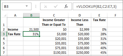
The fourth argument is empty, so the function returns an approximate match. If it didn’t, you’d have to enter one of the values in columns C or D to get a result at all.
When you’re comfortable with VLOOKUP, the HLOOKUP function is equally easy to use. You enter the same arguments, but it searches in rows instead of columns.
Using INDEX and MATCH instead of VLOOKUP
There are certain limitations with using VLOOKUP—the VLOOKUP function can only look up a value from left to right. This means that the column containing the value you look up should always be located to the left of the column containing the return value. Now if your spreadsheet isn’t built this way, then do not use VLOOKUP. Use the combination of INDEX and MATCH functions instead.
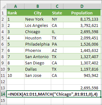
This example shows a small list where the value we want to search on, Chicago, isn’t in the leftmost column. So, we can’t use VLOOKUP. Instead, we’ll use the MATCH function to find Chicago in the range B1:B11. It’s found in row 4. Then, INDEX uses that value as the lookup argument, and finds the population for Chicago in the 4th column (column D). The formula used is shown in cell A14.
For more examples of using INDEX and MATCH instead of VLOOKUP, see the article https://www.mrexcel.com/excel-tips/excel-vlookup-index-match/ by Bill Jelen, Microsoft MVP.
Give it a try
If you want to experiment with lookup functions before you try them out with your own data, here’s some sample data.
VLOOKUP Example at work
Copy the following data into a blank spreadsheet.
Tip: Before you paste the data into Excel, set the column widths for columns A through C to 250 pixels, and click Wrap Text ( Home tab, Alignment group).
Источник
LOOKUP function
Use LOOKUP, one of the lookup and reference functions, when you need to look in a single row or column and find a value from the same position in a second row or column.
For example, let’s say you know the part number for an auto part, but you don’t know the price. You can use the LOOKUP function to return the price in cell H2 when you enter the auto part number in cell H1.
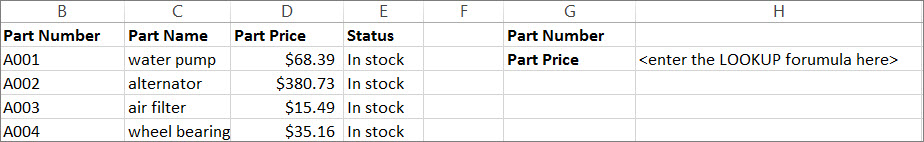
Use the LOOKUP function to search one row or one column. In the above example, we’re searching prices in column D.
Tips: Consider one of the newer lookup functions, depending on which version you are using.
Use VLOOKUP to search one row or column, or to search multiple rows and columns (like a table). It’s a much improved version of LOOKUP. Watch this video about how to use VLOOKUP.
If you are using Microsoft 365, use XLOOKUP — it’s not only faster, it also lets you search in any direction (up, down, left, right).
There are two ways to use LOOKUP: Vector form and Array form
Vector form: Use this form of LOOKUP to search one row or one column for a value. Use the vector form when you want to specify the range that contains the values that you want to match. For example, if you want to search for a value in column A, down to row 6.
Array form: We strongly recommend using VLOOKUP or HLOOKUP instead of the array form. Watch this video about using VLOOKUP. The array form is provided for compatibility with other spreadsheet programs, but it’s functionality is limited.
An array is a collection of values in rows and columns (like a table) that you want to search. For example, if you want to search columns A and B, down to row 6. LOOKUP will return the nearest match. To use the array form, your data must be sorted.
Vector form
The vector form of LOOKUP looks in a one-row or one-column range (known as a vector) for a value and returns a value from the same position in a second one-row or one-column range.
Syntax
LOOKUP(lookup_value, lookup_vector, [result_vector])
The LOOKUP function vector form syntax has the following arguments:
lookup_value Required. A value that LOOKUP searches for in the first vector. Lookup_value can be a number, text, a logical value, or a name or reference that refers to a value.
lookup_vector Required. A range that contains only one row or one column. The values in lookup_vector can be text, numbers, or logical values.
Important: The values in lookup_vector must be placed in ascending order: . -2, -1, 0, 1, 2, . A-Z, FALSE, TRUE; otherwise, LOOKUP might not return the correct value. Uppercase and lowercase text are equivalent.
result_vector Optional. A range that contains only one row or column. The result_vector argument must be the same size as lookup_vector. It has to be the same size.
If the LOOKUP function can’t find the lookup_value, the function matches the largest value in lookup_vector that is less than or equal to lookup_value.
If lookup_value is smaller than the smallest value in lookup_vector, LOOKUP returns the #N/A error value.
Vector examples
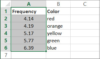
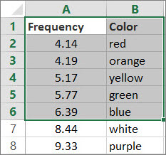
You can try out these examples in your own Excel worksheet to learn how the LOOKUP function works. In the first example, you’re going to end up with a spreadsheet that looks similar to this one:
Copy the data in following table, and paste it into a new Excel worksheet.
Copy this data into column A
Copy this data into column B
Next, copy the LOOKUP formulas from the following table into column D of your worksheet.
Copy this formula into the D column
Here’s what this formula does
Here’s the result you’ll see
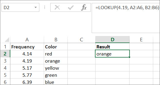
=LOOKUP(4.19, A2:A6, B2:B6)
Looks up 4.19 in column A, and returns the value from column B that is in the same row.
=LOOKUP(5.75, A2:A6, B2:B6)
Looks up 5.75 in column A, matches the nearest smaller value (5.17), and returns the value from column B that is in the same row.
=LOOKUP(7.66, A2:A6, B2:B6)
Looks up 7.66 in column A, matches the nearest smaller value (6.39), and returns the value from column B that is in the same row.
=LOOKUP(0, A2:A6, B2:B6)
Looks up 0 in column A, and returns an error because 0 is less than the smallest value (4.14) in column A.
For these formulas to show results, you may need to select them in your Excel worksheet, press F2, and then press Enter. If you need to, adjust the column widths to see all the data.
Array form
Tip: We strongly recommend using VLOOKUP or HLOOKUP instead of the array form. See this video about VLOOKUP; it provides examples. The array form of LOOKUP is provided for compatibility with other spreadsheet programs, but its functionality is limited.
The array form of LOOKUP looks in the first row or column of an array for the specified value and returns a value from the same position in the last row or column of the array. Use this form of LOOKUP when the values that you want to match are in the first row or column of the array.
Syntax
The LOOKUP function array form syntax has these arguments:
lookup_value Required. A value that LOOKUP searches for in an array. The lookup_value argument can be a number, text, a logical value, or a name or reference that refers to a value.
If LOOKUP can’t find the value of lookup_value, it uses the largest value in the array that is less than or equal to lookup_value.
If the value of lookup_value is smaller than the smallest value in the first row or column (depending on the array dimensions), LOOKUP returns the #N/A error value.
array Required. A range of cells that contains text, numbers, or logical values that you want to compare with lookup_value.
The array form of LOOKUP is very similar to the HLOOKUP and VLOOKUP functions. The difference is that HLOOKUP searches for the value of lookup_value in the first row, VLOOKUP searches in the first column, and LOOKUP searches according to the dimensions of array.
If array covers an area that is wider than it is tall (more columns than rows), LOOKUP searches for the value of lookup_value in the first row.
If an array is square or is taller than it is wide (more rows than columns), LOOKUP searches in the first column.
With the HLOOKUP and VLOOKUP functions, you can index down or across, but LOOKUP always selects the last value in the row or column.
Important: The values in array must be placed in ascending order: . -2, -1, 0, 1, 2, . A-Z, FALSE, TRUE; otherwise, LOOKUP might not return the correct value. Uppercase and lowercase text are equivalent.
Источник
Use Excel built-in functions to find data in a table or a range of cells
Summary
This step-by-step article describes how to find data in a table (or range of cells) by using various built-in functions in Microsoft Excel. You can use different formulas to get the same result.
Create the Sample Worksheet
This article uses a sample worksheet to illustrate Excel built-in functions. Consider the example of referencing a name from column A and returning the age of that person from column C. To create this worksheet, enter the following data into a blank Excel worksheet.
You will type the value that you want to find into cell E2. You can type the formula in any blank cell in the same worksheet.
Term Definitions
This article uses the following terms to describe the Excel built-in functions:
The whole lookup table
The value to be found in the first column of Table_Array.
Lookup_Array
-or-
Lookup_Vector
The range of cells that contains possible lookup values.
The column number in Table_Array the matching value should be returned for.
3 (third column in Table_Array)
Result_Array
-or-
Result_Vector
A range that contains only one row or column. It must be the same size as Lookup_Array or Lookup_Vector.
A logical value (TRUE or FALSE). If TRUE or omitted, an approximate match is returned. If FALSE, it will look for an exact match.
This is the reference from which you want to base the offset. Top_Cell must refer to a cell or range of adjacent cells. Otherwise, OFFSET returns the #VALUE! error value.
This is the number of columns, to the left or right, that you want the upper-left cell of the result to refer to. For example, «5» as the Offset_Col argument specifies that the upper-left cell in the reference is five columns to the right of reference. Offset_Col can be positive (which means to the right of the starting reference) or negative (which means to the left of the starting reference).
Functions
LOOKUP()
The LOOKUP function finds a value in a single row or column and matches it with a value in the same position in a different row or column.
The following is an example of LOOKUP formula syntax:
The following formula finds Mary’s age in the sample worksheet:
The formula uses the value «Mary» in cell E2 and finds «Mary» in the lookup vector (column A). The formula then matches the value in the same row in the result vector (column C). Because «Mary» is in row 4, LOOKUP returns the value from row 4 in column C (22).
NOTE: The LOOKUP function requires that the table be sorted.
For more information about the LOOKUP function, click the following article number to view the article in the Microsoft Knowledge Base:
VLOOKUP()
The VLOOKUP or Vertical Lookup function is used when data is listed in columns. This function searches for a value in the left-most column and matches it with data in a specified column in the same row. You can use VLOOKUP to find data in a sorted or unsorted table. The following example uses a table with unsorted data.
The following is an example of VLOOKUP formula syntax:
The following formula finds Mary’s age in the sample worksheet:
The formula uses the value «Mary» in cell E2 and finds «Mary» in the left-most column (column A). The formula then matches the value in the same row in Column_Index. This example uses «3» as the Column_Index (column C). Because «Mary» is in row 4, VLOOKUP returns the value from row 4 in column C (22).
For more information about the VLOOKUP function, click the following article number to view the article in the Microsoft Knowledge Base:
INDEX() and MATCH()
You can use the INDEX and MATCH functions together to get the same results as using LOOKUP or VLOOKUP.
The following is an example of the syntax that combines INDEX and MATCH to produce the same results as LOOKUP and VLOOKUP in the previous examples:
The following formula finds Mary’s age in the sample worksheet:
The formula uses the value «Mary» in cell E2 and finds «Mary» in column A. It then matches the value in the same row in column C. Because «Mary» is in row 4, the formula returns the value from row 4 in column C (22).
NOTE: If none of the cells in Lookup_Array match Lookup_Value («Mary»), this formula will return #N/A.
For more information about the INDEX function, click the following article number to view the article in the Microsoft Knowledge Base:
OFFSET() and MATCH()
You can use the OFFSET and MATCH functions together to produce the same results as the functions in the previous example.
The following is an example of syntax that combines OFFSET and MATCH to produce the same results as LOOKUP and VLOOKUP:
This formula finds Mary’s age in the sample worksheet:
The formula uses the value «Mary» in cell E2 and finds «Mary» in column A. The formula then matches the value in the same row but two columns to the right (column C). Because «Mary» is in column A, the formula returns the value in row 4 in column C (22).
For more information about the OFFSET function, click the following article number to view the article in the Microsoft Knowledge Base:
Источник
Summary
This step-by-step article describes how to find data in a table (or range of cells) by using various built-in functions in Microsoft Excel. You can use different formulas to get the same result.
Create the Sample Worksheet
This article uses a sample worksheet to illustrate Excel built-in functions. Consider the example of referencing a name from column A and returning the age of that person from column C. To create this worksheet, enter the following data into a blank Excel worksheet.
You will type the value that you want to find into cell E2. You can type the formula in any blank cell in the same worksheet.
|
A |
B |
C |
D |
E |
||
|
1 |
Name |
Dept |
Age |
Find Value |
||
|
2 |
Henry |
501 |
28 |
Mary |
||
|
3 |
Stan |
201 |
19 |
|||
|
4 |
Mary |
101 |
22 |
|||
|
5 |
Larry |
301 |
29 |
Term Definitions
This article uses the following terms to describe the Excel built-in functions:
|
Term |
Definition |
Example |
|
Table Array |
The whole lookup table |
A2:C5 |
|
Lookup_Value |
The value to be found in the first column of Table_Array. |
E2 |
|
Lookup_Array |
The range of cells that contains possible lookup values. |
A2:A5 |
|
Col_Index_Num |
The column number in Table_Array the matching value should be returned for. |
3 (third column in Table_Array) |
|
Result_Array |
A range that contains only one row or column. It must be the same size as Lookup_Array or Lookup_Vector. |
C2:C5 |
|
Range_Lookup |
A logical value (TRUE or FALSE). If TRUE or omitted, an approximate match is returned. If FALSE, it will look for an exact match. |
FALSE |
|
Top_cell |
This is the reference from which you want to base the offset. Top_Cell must refer to a cell or range of adjacent cells. Otherwise, OFFSET returns the #VALUE! error value. |
|
|
Offset_Col |
This is the number of columns, to the left or right, that you want the upper-left cell of the result to refer to. For example, «5» as the Offset_Col argument specifies that the upper-left cell in the reference is five columns to the right of reference. Offset_Col can be positive (which means to the right of the starting reference) or negative (which means to the left of the starting reference). |
Functions
LOOKUP()
The LOOKUP function finds a value in a single row or column and matches it with a value in the same position in a different row or column.
The following is an example of LOOKUP formula syntax:
=LOOKUP(Lookup_Value,Lookup_Vector,Result_Vector)
The following formula finds Mary’s age in the sample worksheet:
=LOOKUP(E2,A2:A5,C2:C5)
The formula uses the value «Mary» in cell E2 and finds «Mary» in the lookup vector (column A). The formula then matches the value in the same row in the result vector (column C). Because «Mary» is in row 4, LOOKUP returns the value from row 4 in column C (22).
NOTE: The LOOKUP function requires that the table be sorted.
For more information about the LOOKUP function, click the following article number to view the article in the Microsoft Knowledge Base:
How to use the LOOKUP function in Excel
VLOOKUP()
The VLOOKUP or Vertical Lookup function is used when data is listed in columns. This function searches for a value in the left-most column and matches it with data in a specified column in the same row. You can use VLOOKUP to find data in a sorted or unsorted table. The following example uses a table with unsorted data.
The following is an example of VLOOKUP formula syntax:
=VLOOKUP(Lookup_Value,Table_Array,Col_Index_Num,Range_Lookup)
The following formula finds Mary’s age in the sample worksheet:
=VLOOKUP(E2,A2:C5,3,FALSE)
The formula uses the value «Mary» in cell E2 and finds «Mary» in the left-most column (column A). The formula then matches the value in the same row in Column_Index. This example uses «3» as the Column_Index (column C). Because «Mary» is in row 4, VLOOKUP returns the value from row 4 in column C (22).
For more information about the VLOOKUP function, click the following article number to view the article in the Microsoft Knowledge Base:
How to Use VLOOKUP or HLOOKUP to find an exact match
INDEX() and MATCH()
You can use the INDEX and MATCH functions together to get the same results as using LOOKUP or VLOOKUP.
The following is an example of the syntax that combines INDEX and MATCH to produce the same results as LOOKUP and VLOOKUP in the previous examples:
=INDEX(Table_Array,MATCH(Lookup_Value,Lookup_Array,0),Col_Index_Num)
The following formula finds Mary’s age in the sample worksheet:
=INDEX(A2:C5,MATCH(E2,A2:A5,0),3)
The formula uses the value «Mary» in cell E2 and finds «Mary» in column A. It then matches the value in the same row in column C. Because «Mary» is in row 4, the formula returns the value from row 4 in column C (22).
NOTE: If none of the cells in Lookup_Array match Lookup_Value («Mary»), this formula will return #N/A.
For more information about the INDEX function, click the following article number to view the article in the Microsoft Knowledge Base:
How to use the INDEX function to find data in a table
OFFSET() and MATCH()
You can use the OFFSET and MATCH functions together to produce the same results as the functions in the previous example.
The following is an example of syntax that combines OFFSET and MATCH to produce the same results as LOOKUP and VLOOKUP:
=OFFSET(top_cell,MATCH(Lookup_Value,Lookup_Array,0),Offset_Col)
This formula finds Mary’s age in the sample worksheet:
=OFFSET(A1,MATCH(E2,A2:A5,0),2)
The formula uses the value «Mary» in cell E2 and finds «Mary» in column A. The formula then matches the value in the same row but two columns to the right (column C). Because «Mary» is in column A, the formula returns the value in row 4 in column C (22).
For more information about the OFFSET function, click the following article number to view the article in the Microsoft Knowledge Base:
How to use the OFFSET function
Need more help?
Want more options?
Explore subscription benefits, browse training courses, learn how to secure your device, and more.
Communities help you ask and answer questions, give feedback, and hear from experts with rich knowledge.
I have 9 columns with names in them and a list of 400 names. How do I populate the column numbers associated with each name without having to go through each name location individually. Kindly advice.

This is an example of what I am looking for. Get the column numbers for a list of names I have in a column.
asked Oct 26, 2018 at 14:47
![]()
The Last WordThe Last Word
1591 gold badge1 silver badge8 bronze badges
3
Use AGGREGATE()
=AGGREGATE(15,6,COLUMN($A$2:$H$4)/($A$2:$H$4=K2),1)
This will create an array of column numbers and #DIV/0 errors. The AGGREGATE will ignore the errors and return the lowest column number where the value is found.

answered Oct 26, 2018 at 15:06
![]()
Scott CranerScott Craner
22.2k3 gold badges21 silver badges24 bronze badges
sample files
1. ADDRESS Function
The ADDRESS Function returns a valid cell reference as per the column and row address. In simple words, you can create an address of a cell by using its row number and column number.
Syntax
ADDRESS(row_num,column_num,abs_num,A1,sheet_text)
Arguments
- row_num: A number to specify row number.
- column_num: A number to specify column number.
- [abs_num]: Reference type.
- [A1]: Reference style.
- [sheet_text]: A text value as a sheet name.
Notes
- By default, the ADDRESS function returns absolute reference in the result.
Example
In the below example, we have used different arguments to get all types of results.

With R1C1 reference style:
- Relative reference.
- Relative row and absolute column reference.
- Absolute row and relative column reference.
- Absolute reference.
With A1 reference style:
- Relative reference.
- Relative row and absolute column reference.
- Absolute row and relative column reference.
- Absolute reference.
2. AREAS Function
The AREAS Function returns a number that represents the number of ranges in the reference you have specified. In simple words, it actually counts the different worksheet areas you have referred to the function.
syntax
AREAS(reference)
Arguments
- reference: A Reference to a cell or a range of cells.
Notes
- Reference can be a cell, a range of cells or a named range.
- If you want to refer to more than one cell reference, you have to enclose all those references in more than one set of parentheses and use commas to separate each reference from others.
Example
In the below example, we have used areas function to get the number reference in a named range.

As you can see there are three columns in the range and it has returned 3 in the result.

3. CHOOSE Function
The CHOOSE function returns a value from the list of values based on the position number specified. In simple words, it looks for a value from a list based on its position and returns it in the result.
Syntax
CHOOSE(index_num,value1,value2,…)
Arguments
- index_num: A number for specifying the position of the value in the list.
- value1: A range of cells or an input value from which you can choose.
- [value2]: A range of cells or an input value from which you can choose.
Notes
- You can refer to a cell or you can also insert values directly in the function.
Example
In the below example, we have used CHOOSE function with a drop-down list to calculate four(sum, average, max, and mix) different things. So, we have used the below formula to calculate all four things:
=CHOOSE(VLOOKUP(K2,Q1:R4,2,FALSE),SUM(O2:O9),AVERAGE(O2:O9),MAX(O2:O9),MIN(O2:O9))

We have this small table with the name of all four calculations which we want and a serial number to each in the corresponding cell.
After that, we have a drop-down list for all four calculations. Now, to get index number in the choose function from that small table we have a lookup formula which will returns serial number as per the value selected from the drop-down list.
And instead of values, we have used four formulas for 4 different calculations.
4. COLUMN Function
The COLUMN function returns the column number for the given cell reference. As you know, every cell reference is made up of a column number and a row number. So it takes the column number and returns it in the result.
Syntax
COLUMN([reference])
Arguments
- reference: A cell reference for which you want to get the column number.
Notes
- You cannot refer to multiple references.
- If you refer to an array, the column function will also return the column numbers in an array.
- If you refer to a range of more than one cell, it will return the column number of the leftmost cell. For example, if you refer to the range A1:C10, it will return the column number of the cell A1.
- If you skip specifying a reference, it will return the column number of the current cell.
Example
In the below example, we have used COLUMN to get the column number of the cell A1.

As I have already mentioned, if you skip specifying cell reference it will return the column number of the current cell. In the below example, we have used COLUMN to create a header with serial numbers.

5. COLUMNS Function
The COLUMNS function returns the number of columns referred to in the given reference. In simple words, it counts how many columns are there in the supplied range and returns that count.
Syntax
COLUMNS(array)
Arguments
- array: An array or range of cells from which you want to get the number of columns.
Notes
- You can also use a named range.
- COLUMNS function is not concerned with the values in the cells, it will simply return the number of columns in a reference.
Example
In the below example, we have used COLUMN to get the number of columns from range A1:F1.

6. FORMULATEXT Function
The FORMULATEXT function returns the formula from the referred cell. And if there’s no formula in the referred cell, a value, or a blank, it will return a #N/A.
Syntax
FORMULATEXT(reference)
Arguments
- reference: The cell reference from which you want formula as a text.
Notes
- If you refer to another workbook that workbook should be open, otherwise it will not show the formula.
- If you refer to a range more than a single cell, it will return formula from the upper-left cell of the given range.
- It will return an “#N/A” error value if the cell you are using as a reference does not contain any formula, has a formula with more than 8192 characters, a cell is protected, or an external workbook is not opened.
- If you refer two cells in circular reference it will return results from both.
Example
In the below example, we have used formula text with different types of references. When you refer to a cell that doesn’t have any formula, it will return “#N/A” error value.

7. HLOOKUP Function
The HLOOKUP function lookups for a value in the top row of a table and returns the value from the same column of the matched value using the index number. In simple words, it performs a horizontal lookup.
Syntax
HLOOKUP(lookup_value, table_array, row_index_num, [range_lookup])
Arguments
- lookup_value: The value you want to lookup.
- table_array: The data table or an array from which you want to the lookup value.
- row_index_num: A numeric value representing a number of rows below from the top row from which you want the value. For example, if you specify 2 and your lookup value is in A10 in the data table, it will return value from cell B10.
- [range_lookup]: A logical value to specify the type of lookup. If you want to perform an exact match search use FALSE and if you want to perform a non-exact match use TRUE (Default).
Notes
- You can use wildcard characters.
- You can perform an exact match and an approximate match.
- While performing an approximate match make sure to sort data in ascending order from left to right, and if data is not in ascending order then it would return an inaccurate result.
- If range_lookup is true or omitted, it will perform a non-exact match but return an exact match if the lookup value exists in the lookup range.
- If range_lookup is true or omitted, and the lookup value is not in the lookup range, it will return the nearest value which is less than the lookup value.
- If range_lookup is false, then there is no need to sort data range.
Example
In the below example, we have used the HLOOKUP function with MATCH to create a dynamic formula and then we have used a drop-down list to change the lookup value from the cell.

The zone name from cell C7 is used as a lookup value. Range B1: F5 as table array and for row_index_num we have used match function to get the row number.

Whenever you change the value in cell C9, it will return the row number from the table array. You don’t have to change your formula again and again. Just change values with the drop-down list and you will get value for that.
8. HYPERLINK Function
The HYPERLINK function returns a string with a hyperlink attached to it. In simple words, like the HYPERLINK option you have in Excel, the HYPERLINK function helps you to create a hyperlink.
Syntax
HYPERLINK(link_location,[friendly_name])
Arguments
- Link_Location: The location for which you want to add a HYPERLINK. It can be further split into two terms.
- link: It can be an address of a cell or range of cells in the same worksheet or in any other worksheet or in any other workbook. We can also link a bookmark from a word document.
- location: It can be a link to a hard drive, a server using the UNC path, or any URL from the internet or intranet. (In Excel online you can only use web address for HYPERLINK function). You can insert a link to the function by inserting it as a text with quotation marks or by referring to a cell containing the link as a text. Make sure to use “HTTPS://” before a web address.
- [friendly_name]: It is an optional part of this function. It acts as the face of the connecting link.
- You can use any type of text, number, or both.
- You also refer to a cell which contains the friendly_name.
- If you skip it, the function will use the link address to display.
- If friendly_name returns an error, the function will display error.
Notes
- Link a file saved on a Web Address: You can use a file that is saved on a web address. This helps us to share the file in an effective way.
- Link a file saved on a Hard Drive: You can also use this function while working offline. You can link a file that is stored on your hard drive and access them through your single excel sheet, no need to go to every single folder to open them.
- Link a Word Document File: This is also an awesome feature of HYPERLINK function. You can link a Word document file or a specific place in word document file using a bookmark.
- Link a file without using Friendly Name: If you want to show the actual link to the file or place to the user. In this situation, you just need to skip the friendly name declaration in the HYPERLINK Function.
9. INDEX Function
The INDEX function returns a value from a list of values based on its index number. In simple words, INDEX returns a value from a list of values and you need to specify that value’s position.
Syntax
INDEX has two different syntaxes.
In the first, you can use an array form of an index to simply get a value from a list using its position.
INDEX(array, row_num, [column_num])
In the second, you can use a referral form that is less used in real life but you can use it if you have more than one range to get value from.
INDEX(reference, row_num, [column_num], [area_num])
Arguments
- array: A range of cells or an array constant.
- reference: A range of cells or multiple ranges.
- row_number: The number of the row from which you want to get the value.
- [col_number]: The number of the column from which you want to get the value.
- [area_number]: If you are referring to more than one range of cells (using reference syntax), specify a number to refer to a range from all those.
Notes
- When both the row_num and column_num arguments are specified, it will return the value in the cell at the intersection of both.
- If you specify row_num or column_num as 0 (zero), it will return the array of values for the entire column or row, respectively.
- When row_num and column_num are out the range, it will return an error #REF!.
- If area_number is greater than the number ranges you have specified then it will return #REF!.
Example
1. Using ARRAY – Getting Value from a List
In the below example, we have used the INDEX function to get the quantity of June month. In the list, Jun is in 6th position (6th row) that’s why I have specified 6 in row_number. INDEX has returned the value 1904 in the result.

And if you referring to a range with more than one column you have to specify the column number.
2. Using REFERENCE – Getting Value from Multiple Lists
In the below example, instead of selecting all the range in one go, I have selected it as three different ranges. In the last argument, we have specified 2 in area_number which will define the range to use from these three different ranges.

Now in the second range, we are referring to the 5th row and 1st column. INDEX has returned the value 172 which in the 5th row in the 2nd range.
10. INDIRECT Function
The INDIRECT function returns a valid reference from a text string which represents a cell reference. In simple words, you can refer to a cell range by using the cell address as a text value.
Syntax
INDIRECT(ref_text, [a1])
Arguments
- ref_text: A text which represents the address of a cell, an address of a range of cells, a named range, or a table name. For example, A1, B10:B20, or MyRange.
- [a1]: A number or a boolean value to represent the type of cell reference you are specifying in ref_text. For example, if you want to use A1 reference style use TRUE or 1 and if you want to use R1C1 reference style use FALSE or 0 for R1C reference style. And if you omit to specify the cell reference type, it will use A1 style as default.
Notes
- When you referred to another workbook, that workbook should be opened.
- If you insert a row or a column in the range which you have referred, INDIRECT will not update that reference.
- If you want to insert text directly into the function you have to put it in double quotation marks or you can also refer to a cell that has the text you want to use as a reference.
Example
1. Reference to Another Worksheet
You can also refer to another worksheet using the INDIRECT and you have to insert the worksheet name in it. In the below example, we have used the indirect function to refer to another worksheet and have the sheet name in cell A2 and cell reference in cell B2.

In cell C2, we have used the following formula to combine the text.
=INDIRECT(“‘”&A2&”‘!”&B2)
This combination creates a text which is used by the INDIRECT function to refer to the cell A1 in sheet1 and the best part is when you change the worksheet name or cell address the reference will automatically change.
Cell A1 in “Sheet1” has the value “Yes” and that’s why indirect returns the value “Yes”.
2. Reference to Another Workbook
You can also refer to another workbook, in the same way, we did for another worksheet. All you have to do, just add a workbook name in your text which you are using as a reference.

In the above example, we have used the following formula to get the value from the cell A1 of the workbook “Book1”.
=INDIRECT(“[“&A2&”]”&B2&”!”&C2)
As we have the workbook name in cell “A2”, worksheet name in cell “B2” and cell name in cell “C2”. We have combined them to use as an input text in indirect function.
Note: While combining cell reference as a text make sure to follow the right reference structure.
3. Using with Named Ranges
Yes, you can also refer to a named range using the indirect function. It’s just simple. Once you create a named range you have to enter that named range as a text in INDIRECT.

In the above example, we have a drop-down in cell E1 which has a list of named ranges, and in cell E2 we have used that name. As range B2:B5 is named as “Quantity” and range C2:C5 is named as “Amount”.
When you select quantity from drop-down indirect function instantly refers to the named range. And when you select the amount from the drop-down, you will have the sum of cell range C2:C5.
11. LOOKUP Function
The LOOKUP function returns a value (which you are looking up) from a row, column, or from an array. In simple words, you can look up for a value, and LOOKUP will return that value if it’s there in that row, column, or array.
Syntax
LOOKUP(value, lookup_range, [result_range])
There are two types of LOOKUP functions.
- Vector Form
- Array Form
Arguments
- value: The value that you want to search from a column or a row.
- lookup_range: The column or row from which you want to lookup for the value.
- [result_range]: The column or row from which you want to return a value. This is an optional argument.
Notes
- Instead of using array form it’s better to use VLOOKUP or HLOOKUP.
12. MATCH Function
The MATCH function returns the index number of the value from an array. In simple words, the MATCH function looks up for a value in the list and returns the position number of that value in the list.
Syntax
MATCH (lookup_value, lookup_array, [match_type])
Arguments
- lookup_value: The value whose position you want to get from a list of values.
- lookup_array: The range of cell or an array contains values.
- [match_type]: The number (-1, 0 & 1) to specify how excel look for the value from the list of values.
- If you use 1, it will return the largest value which is equal or less than the lookup value. The values in the list must be sorted in ascending order.
- If you use -1, it will return the smallest value which is equal or greater than the lookup value. The values in the list must be sorted in ascending order.
- If you use 0, it will return the exact match from the list.
Notes
- You can use wildcard characters.
- If there is no matching value in the list if will return #N/A.
- The match function is non-case sensitive.
Example
In the below example, we have used 1 as match type and we are looking for value 5.

As I have already mentioned if you use 1 in match type it returns the largest value which is equal or smaller than the lookup value. In the entire list, there are 3 values that are smaller than 5 and 4 is the highest in them.
That’s why in the result it has returned 3 which is the position of value 4.
13. OFFSET Function
The OFFSET function returns a reference to a range which is a specific number of rows and columns away from a cell or range of cells. In simple words, you can refer to a cell or a range of cells by using rows and columns from a starting cell.
Syntax
OFFSET(reference, rows, cols, [height], [width])
Arguments
- reference: The reference from which you want to offset to start. It can be a cell or range of adjacent cells.
- rows: The number of rows that tell OFFSET to move up or down from the reference. To go downward you need a positive number and for going upwards you need a negative number.
- cols: The number of columns tells OFFSET to move to the left or right from the reference. To go right you need a positive number and for going left you need a negative number.
- [height]: A number to specify the rows to include in the reference.
- [width]: A number to specify the columns to include in the reference.
Notes
- OFFSET is a “volatile” function, it recalculates whenever there is any change to a worksheet.
- It displays the #REF! error value if the offset is outside the edge of the worksheet.
- If height or width is omitted, the height and width of reference are used.
Example
In the below example, we have used SUM with OFFSET to create a dynamic range which sums the values from all the months for a particular product.

14. ROW Function
The ROW function returns the row number of the referred cell. In simple words, with the ROW function, you can get the row number of a cell and if you don’t refer to any cell then it returns the row number for the cell where you insert it.
Syntax
ROW([reference])
Arguments
- reference: A cell reference or a range of cells for which you want to check the row number.
Notes
- It will include all types of sheets (Chart Sheet, Worksheet or Macro Sheet).
- You can refer to sheets even if they are visible, hidden or very hidden.
- If you skip specifying any value in the function it will give you the sheet number of the sheet in which you have applied the function.
- If you specify an invalid sheet name, it will return a #N/A.
- If you specify an invalid sheet reference, it will return a #REF!.
Example
In the below example, we have used the row function check the row number of the same cell where we have used the function.

In the below example, we have referred to another cell to get the row number of that cell.

You can use the row function to create a serial number list in your worksheet. All you have to do is just enter row functions in a cell and drag it up to the cell you want to add serial numbers.

15. ROWS Function
The ROWS function returns a count of the rows from the referred range. In simple words, with the ROWS function you can count how many rows are in the range you have referred to.
Syntax
ROWS(array)
Arguments
- array: A cell reference or an array to check the number of rows.
Notes
- You can also use a named range.
- It is not concerned with the values in the cells, it will simply return the number of rows in a reference.
Example
In the below example, we have referred to a vertical range of 10 cells and it has returned 10 in the result as the range includes 10 rows.

16. TRANSPOSE Function
The TRANSPOSE function changes the orientation of a range. In simple words, by using this function you can change the data from a row into a column and from a column into a row.
Syntax
TRANSPOSE (array)
Arguments
- array: An array or a range you want to transpose.
Notes
- You have to apply TRANSPOSE as an array function, using the same number of cells as you have in your source range by pressing Ctrl + Shift + Enter.
- If you select cells less than source range, it will transpose data only for those cells.
Example
Here we need to transpose data from range B2:D4 to range G2 to I4:

For this, first, we need to go to the cell G2 and select cell range up to I4.

Next is to enter (=TRANSPOSE(B2:D4)) in cell G2 and press Ctrl+Shift+Enter.

TRANSPOSE will convert the data from the rows into columns, and the formula which we have applied is an array formula, you cannot change a single cell from it.

17. VLOOKUP Function
The VLOOKUP function lookups for a value in the first column of a table and returns the value from the same row of the matched value using the index number. In simple words, it performs a vertical lookup.
Syntax
VLOOKUP(lookup_value,table_array,col_index_num,range_lookup)
Arguments
- lookup_value: A value that you want to search in a column. You can refer to a cell that has the lookup value or you can directly enter that value into the function.
- table_array: A range of cells, a named range from which you want to look up the value.
- col_index_num: A number represents the column number from which you want to retrieve the value.
- range_lookup: Use false or 0 to make an exact match and true or 1 for an appropriate match. The default is True.
Notes
- If VLOOKUP cannot find the value you are looking for, it will return an #N/A.
- VLOOKUP is only able to give you the value which is on the right side of the lookup value. If you want to look upon the right side, you can use INDEX and MATCH for that.
- If you are using an exact match then it will only match the value which is first in the column.
- You can also use wildcard characters with VLOOKUP.
- You can use TRUE or 1 if you want an appropriate match and FALSE or 0 for an exact match.
- If you are using an appropriate match (True): It will return the next smallest value from the list if there is no exact match.
- If the value which you are looking for is smaller than the smallest value in the list, VLOOKUP will return #N/A.
- If there is an exact value exists which you are looking for, it will give you that exact value.
- Make sure you have sorted the list in ascending order.
Example
1. Using VLOOKUP for Categories
In the below example, we have a list of students with marks they have scored, and in the remarks column, we want to a grade according to their marks.

In the above marks list, we want to add remarks as per the below category range.

In this, we have two options to use.
FIRST is to create a nesting formula with IF which is a little bit time-consuming, and the SECOND option is to create a formula with VLOOKUP with an appropriate match. And, the formula will be:
=VLOOKUP(B2,$E$2:$G$5,3,TRUE)

How it works
I am using the “MIN MARKS” column to match the lookup value and I am getting value in return from the “Remarks” column.
I have already mentioned that when you use TRUE and there is no exact match lookup value then it will return the next smallest value from the lookup value. For example, when we are looking for a value 77 from the category table, 65 is the next smallest value after 77.
That is why we got “Good” in remarks.
2. Handling Errors in VLOOKUP Function
One of the most common problems which come when you are using VLOOKUP is that you’ll get #N/A whenever there is no match is found by it. But the solution to this problem is simple and easy. Let me show with an easy example.
In the below example, we have a list of names and their age and in cell E6, we are using the VLOOKUP function to look up a name from the list. Whenever I type a name that is not on the list I am getting #N/A.

But what I want here is to show a meaningful message instead of the error. The formula will be: =IFNA(VLOOKUP(D6,Sheet3!$A$1:$B$14,2,0),”Not Found”)

How it works: IFNA can test a value for #N/A and if there is an error you can specify a value instead of the error.
Here is a way to do it with formulas. I’ll show how to do it with a few different formulas to show the steps of the logic, and then put them together into one big formula.
First, use one formula per column to see if the target value is in the column. For example in column A:
=COUNTIF(A1:A100,Goal)
=COUNTIF(B1:B100,Goal)
...
(where Goal can be a hardcoded search value,
 or a named range where you type your query)
Then, add IF statements to these formulas to translate this into column numbers. If the query is present in the column, show the column number, else show zero.
=IF(COUNTIF(A1:A100,Goal)>0, 1, 0)
=IF(COUNTIF(B1:B100,Goal)>0, 2, 0)
...
Finally, add a formula to grab the maximum column number from the prior formulas. This will equal the rightmost column with your query value in it.
=MAX( IF(COUNTIF(A1:A100,Goal)>0, 1, 0), IF(COUNTIF(B1:B100,Goal)>0, 2, 0), ...)